Capabilities and limitations of Large Eddy Simulation with perfectly stirred reactor assumption for engineering applications of unsteady, hydrogen combustion sequences

Abstract

This work evaluates the capabilities of Large Eddy Simulation with perfectly stirred reactor (PSR) assumption and detailed chemistry to predict unsteady, premixed, hydrogen combustion sequences. The model was benchmarked with hydrogen-air experimental tests and with numerical data of flame acceleration in an obstructed channel. Results permit to identify major shortcomings that should be addressed with this approach and to assess the uncertainties linked to the use of different sub-models. Spatial resolution was found to be critical and limits the applications of this approach due to the increase of the computational costs with the flame surface. While the influence of the detailed kinetic chemical scheme used was low, the impact of the sub-grid turbulence model used was high. Results showed that simulations provided good agreement with the experimental data when a minimum spatial resolution of 1/8 of the laminar flame thickness was imposed. This threshold permits to simulate with good results the early stages of the combustion sequence (ignition and initial flame acceleration) but limits the model applications when the flame surface increases. In-situ Adaptive Tabulation (ISAT) was an effective strategy to overcome the limitations and partially reduce the computational cost when detailed chemistry models are used together with PSR-LES.

KEYWORDS:

• Perfectly stirred reactor
• implicit LES
• fast combustion
• unsteady

1. Introduction

Chemical industry (Hoi et al., 2007), nuclear power plants (Garcia-Cascales et al., 2014; Karata et al., 2012; OECD, 2000; Sathiah et al., 2012), propulsion (Roy et al., 2004; Smirnov et al., 1999) are some of the fields where experts are especially concerned about safe combustion, accident prevention or hydrodynamics prediction. Benchmarks and real case studies of applications of computational fluid dynamics (CFD) models are key exercises to improve the knowledge in these fields (Issakhov et al., 2020; Kim & Kim, 2019; Pedersen & Rüther, 2019; Soto-Meca et al., 2016; Xiang et al., 2020). These strategies and others where CFD models are coupled with artificial techniques (Mosavi et al., 2019; Park et al., 2020; Shamshirband et al., 2020) are contributing to enhance the efficiency of the computations in these fields. Mosavi et al. (2019) showed how machine learning can help CFD in the prediction of hydrodynamic parameters on two-phase flow of a bubble column reactor with lower computational costs. Shamshirband et al. (2020) proposed a combination of an artificial intelligence optimization algorithm and CFD for modeling chemical-reactor hydrodynamics. Pedersen and Rüther (2019) used a case study to validate a hybrid CFD model and reduce the uncertainty in the prediction of peak flood discharges in rivers. In their study, the authors built both, a lab-scale model and a mesh grid from the same stereolithographic file of a gauging station located in a river in Norway and validated the simulations with the experimental data obtained from the lab-scale model. Issakhov et al. (2020) studied the chemical reaction of combustion sub-products emitted from a thermal power plant located in Kazakhstan and its dispersion in the nearby of the plant with CFD. They used two benchmarks to validate their CFD model before they applied it to the actual case of the study. Xiang et al. (2020) applied different finite-rate combustion models to transonic combustion test cases and compared the results with reference experimental combustors. This comparison permitted to evaluate their capabilities when modeling turbulence-chemistry interactions in transonic combustors. In H₂ accident prevention, Kim and Kim (2019) developed a CFD model for predicting H₂ detonation accidents in nuclear power plants. They used a Euler approach with a 7-step chemical-kinetics scheme that validated both theoretical transonic tests and lab-scale detonation experiments with good results. After the validation, they applied the model to the containment of a nuclear power plant and evaluated the wall overpressure levels that could be reached if a detonation took place. They found that an inventory of 20% of H₂ in the containment would generate overpressure levels of the order of ∼2 MPa if a detonation sequence happened.

Nowadays, accurate modeling of H₂ combustion on accident sequences in confined scenarios is difficult due to computational costs and the limited ad-hoc experiments available to validate the models. When it comes to validation, turbulence and chemistry are key topics (Xiang et al., 2020). Modeling of these processes together is highly desirable in many high-Reynolds-number problems, to obtain realistic predictions from the numerical results. Large-Eddy Simulations (LES) seems to be a cost-effective method to reach this goal when analyzing H₂ combustion dynamics in accident sequences. A realistic description of this type of combustion sequences requires the model to take into account several important flow mechanisms. Flow instability and wall interaction are key aspects of gas combustion dynamics playing an important role in flame acceleration or quenching. The non-linearity of the advection process leads to instabilities making the flow unsteady and three dimensional (3D). These instabilities, linked with the vortex dynamics, are some of the dominant flow mechanisms leading to the combustion dynamics. During acceleration, interactions between the flame front and the reflections of pressure perturbations in walls and obstacles might enhance heat release rate and vorticity generation due to Richtmyer-Meshkov instability (Ciccarelli et al., 2010; Meshkov, 1969). Several investigations (Ciccarelli et al., 2010), showed that stretching of the flame front due to the interaction with a non-uniform velocity field is one of the main causes of the flame acceleration. Therefore, to obtain a proper prediction of a combustion sequence, correct modeling of turbulence is essential. For problems with high Reynolds number, Direct Numerical Simulation (DNS) is a useful but demanding approach in terms of computational cost. On the contrary, LES is an option that provides results with reasonable accuracy for turbulent combustion (Pitsch, 2006). Another significant aspect that must be considered is the reaction kinetics. Some of the finite-rate combustion approaches which can be found within the LES framework are: the Implicit LES (ILES) (Duwig et al., 2011; Duwig & Dunn, 2013; Duwig & Ludiciani, 2014; Fureby, 2007; Grinstein & Kailasanath, 1995; Krüger et al., 2013), the Thickened Flame Models / Artificially Thickened Flame models (TFM / ATF) (Colin et al., 2000), the Partially Stirred Reactor (PaSR) models (Berglund et al., 2010) or the combustion modeling based on the Eddy Dissipation Concept (EDC) (Giacomazzi et al., 2004). It is also worth citing other models such as the LES Conditional Moment Closure (CMC), that uses conditionally averaged species equations (Navarro-Martinez et al., 2005), the Linear Eddy Model (LEM) which is based on solving 1D problems with high resolution meshes to obtain data required to model the sub-grid variables involved in LES of a 3D problem (Sankaran & Menon, 2005) or Probability/Filtered Density Function (PDF/FDF) models (Raman & Pitsch, 2007). The ILES, sometimes called ‘monotonically integrated’ LES (or MILES), considers that each computational cell has a homogeneous concentration and temperature at sub-grid level. In other words, it considers a perfectly stirred reactor situation within the sub-grid domain (PSR-LES). Thus, the validity of this model depends on the intensity of the sub-grid mixing for the combustion regime considered (Fureby, 2007; Duwig et al., 2011). Previous studies showed ILES was able to predict the burning flame speed of reactive flows which had intense small-scale turbulence (Duwig & Dunn, 2013; Duwig & Ludiciani, 2014; Grinstein & Kailasanath, 1995; Krüger et al., 2013). This is the case for distributed combustion regime (Duwig et al., 2011). For the corrugated flamelet regime, to neglect sub-grid scale contributions of the reaction modeling can be a good strategy when the resolution of the grid applied in LES is enough to resolve flame wrinkling patterns (Fiorina et al., 2015). However, it has limitations if the LES grid resolution is not enough. In practice, this strategy can predict the reaction rate relatively well if the heat loses or the stratification weaken the combustion reaction (what results in the thickening of the flame) or if the flame regime falls within the distributed reaction zone or close to it (Dodoulas & Navarro-Martinez, 2013; Duwig et al., 2012; Grinstein & Kailasanath, 1995). Out of that range, this approach may have limitations that must be identified. In the case of steady/frozen combustion conditions, Fiorina et al. (2015) compared this LES approach with others for a gas burner. In that work, they used a Smagorinski sub-grid scale turbulence model. The authors indicated that the selection of the chemical kinetics scheme also influences the reliability of this approach, as the reaction intermediaries that have shorter characteristic length scales may require finer meshes. They also showed that, in the case of stratified flame conditions, compared to other models, implicit LES exhibited the shortest downstream flame expansion. In that region, the authors found that the grid was not fine enough to capture the wrinkling and thickness of the flame. As a consequence, the under resolution within the flame and the lack of a sub-grid scale flame wrinkling model underestimated the release of heat through the flame front. This resulted in a underprediction of the burning velocity of the flame and its expansion. Nonetheless, under those steady flow conditions, the PSR-LES was able to predict the average flame position in the region of laminar or quasi-transitional flow at the burner base (Fiorina et al., 2015).

As previously commented, PSR-LES model increases its computational requirements as a flame increases its surface, wrinkling and/or it transitions to turbulent regime. These processes eventually result an exponential increase of the computational demands that makes it challenging to fulfill. In this work, it is investigated whether there exists a minimum, flame grid-resolution, criterion that should be imposed in the model in order to fulfill the quality requirements needed to rely on the simulation results. Besides, it is analyzed whether a chemical integration strategy like ISAT could help effectively to overcome this limitation and to reduce the computational demand of this LES approach.

To the author's knowledge, there is a lack of studies in the open literature where the capabilities and drawbacks of the PSR-LES approach are critically assessed to predict unsteady burning speed, and time evolution of other global variables, for example, during the initial stages of transient combustion sequences. Accordingly, this work seeks to evaluate the capabilities and the limitations of implicit LES without sub-grid scale combustion modeling (PSR-LES), coupled with detailed chemical kinetic schemes, to predict global variables of the combustion process. Moreover, it seeks to evaluate the performance of this approach at the initial stage of the combustion sequence (i.e. in the post-ignition, and in the flame acceleration phases, where the flow regime has a low or moderate Reynolds number). This assessment is performed by benchmarking the numerical simulations against combustion experiments performed with hydrogen-air mixtures in a spherical bomb by Sabard et al. (2013), and Goulier, Comandini, et al. (2017). Through this evaluation, the work also seeks to assess the impact of different sub-grid scale models, numerical schemes and chemical kinetic models, when applied in reactive flows in confined scenarios. Besides, numerical data of flame acceleration in an obstructed channel obtained with a different, contrasted, LES approach (i.e. the Artificially Thickened Flame (ATF) sub-grid combustion model), is also used to benchmark this approach.

In section 2, the physical models formulated for the problem studied are presented. These include conservation equations for the gas mixture, condition-dependent heat capacities, and the modeling of turbulence and chemistry with different sub-grid scale models, and chemical kinetics. Secondly, the numerical models are described. In section 3, the model is compared with the results of several experiments carried out in a spherical bomb, and with numerical data of flame acceleration in an obstructed channel. These data were used to identify and discuss the capabilities and drawbacks of this approach in section 4. Finally, in the last section, the conclusions and future work are outlined.

2. Materials and methods: the mathematical model

2.1. Governing equations

The model relies on the multicomponent transport equations of momentum, species mass fractions, and energy, and is closed with an equation of state. The approach used in this work is based on the modeling of turbulence by Large Eddy Simulation. Thus, the governing equations are presented in the Favre-averaged form (Chen et al., 1991) for the conservation of mass, momentum and energy (Equations 1–3) for compressible flow, as well as the transport equations for the species involved in the combustion process (Equation 4): (1) $\begin{array}{rl}& \text{Continuity:}\frac{\mathrm{\partial }\overline{\rho }}{\mathrm{\partial }t}+\mathrm{\nabla }\cdot (\overline{\rho }\tilde{\mathit{u}})=0\end{array}$(1) (2) $\begin{array}{rl}& \text{Momentum}:\frac{\mathrm{\partial }(\overline{\rho }\tilde{\mathit{u}})}{\mathrm{\partial }t}+\mathrm{\nabla }\cdot (\overline{\rho }\tilde{\mathit{u}}\otimes \tilde{\mathit{u}})\\ & =-\mathrm{\nabla }\overline{p}+\mathrm{\nabla }\cdot (\overline{\mathit{S}}-\mathit{B})\end{array}$(2) (3) $\begin{array}{rl}& \text{Energy}:\frac{\mathrm{\partial }\overline{\rho }\widetilde{h_s}}{\mathrm{\partial }t}+\mathrm{\nabla }\cdot (\overline{\rho }\tilde{\mathit{u}}\widetilde{h_s})=\overline{\mathit{S}}\cdot \mathrm{\nabla }\tilde{\mathit{u}}+\frac{\mathrm{\partial }\overline{p}}{\mathrm{\partial }t}+\mathrm{\nabla }\overline{p}\cdot \tilde{\mathit{u}}\\ & +\mathrm{\nabla }\cdot (\overline{\mathit{h}}-{\mathit{b}}_{\mathit{h}})+\overline{\rho }\tilde{\sigma }-\sum _{k=1}^N(\widetilde{{\dot{\omega }}_k}{h}_{f,k}^0)\end{array}$(3) (4) $\begin{array}{rl}& \text{Mass Fraction of species}:\frac{\mathrm{\partial }\overline{\rho }\widetilde{Y_k}}{\mathrm{\partial }t}+\mathrm{\nabla }\cdot (\overline{\rho }\tilde{\mathit{u}}\widetilde{Y_k})\\ & =\mathrm{\nabla }\cdot (\overline{{\mathit{J}}_i^k{Y}_k}-\overline{\rho }(\widetilde{\mathit{u}{Y}_k}-\tilde{\mathit{u}}\widetilde{Y_k}))+\widetilde{{\dot{\omega }}_k}\text{with}\\ & \times k=1,\dots ,\text{ NS}-1\end{array}$(4) where NS is the number of gas species, the $\overline{\cdot }$ and $\tilde{\cdot }$ are, respectively, the Favre Filtered quantities, which fulfill the property: $\overline{\rho }\tilde{\varphi }=\overline{\rho \varphi }$. Thus, $\overline{\rho }$, $\text{and}\tilde{\mathit{u}}$, represents the density of the mixture and the velocity vector, whereas $\widetilde{h_s}$ and $\overline{p}$ stands for the sensible enthalpy and the gas pressure. $h_{f,k}^0$ is the formation enthalpy, and $\widetilde{{\dot{\omega }}_k}$ denotes the filtered reaction rate for the k-th species. The viscous stress tensor is denoted by $\overline{\mathit{S}}$, whereas the heat flux vector is $\overline{\mathit{h}}$ and $\mathit{B}=\overline{\rho }(\widetilde{\mathit{u}\otimes \mathit{u}}-\tilde{\mathit{u}}\otimes \tilde{\mathit{u}})$ is the tensor of unresolved sub-grid stress. ${\mathit{b}}_h=\overline{\rho }(\widetilde{\mathit{u}{h}_s}-\tilde{\mathit{u}}\widetilde{h_s})$ is the vector of unresolved sub-grid heat flux that results when Favre filtering is applied to the convective terms. Besides, it is assumed that $\overline{\mathit{S}}\approx 2\mu \cdot dev(\overline{S})$ and $\overline{\mathit{h}}\approx D_{th}\mathrm{\nabla }\tilde{T}$. Note that $\mu$ is the viscosity and the deviatoric part of the resolved rate strain tensor is denoted by $dev(\overline{S})$, and $D_{th}$ is the thermal diffusivity. Besides, a sub-grid LES model was employed for the unclosed terms for the filtered equations of the momentum and energy conservation.

Regarding the transport of species (Equation 4), the term ${\mathit{J}}_i^k$ is the i-th component of the laminar diffusive flux of species k. This term can be simplified by assuming the approximation of Hirschfelder et al. (1954), and by using Fick’s law, and assuming that the corresponding binary diffusion coefficients are equal (Williams, 1985). That yields: $\mathrm{\nabla }\cdot (\overline{\rho }\tilde{D}\mathrm{\nabla }\widetilde{Y_k})$. This Favre form of the species equation has two unclosed terms which have to be modeled: the unresolved scalar transport term is commonly modeled in LES as $\widetilde{\mathit{u}{Y}_k}-\tilde{\mathit{u}}\widetilde{Y_k}=-{\tilde{D}}_{sgs}\mathrm{\nabla }\widetilde{Y_k}$, with ${\tilde{D}}_{sgs}=\frac{v_{sgs}}{S{c}_t}$, where $v_{sgs}$ is the sub-grid scale turbulent viscosity, and the $S{c}_t$ is the turbulent or sub-grid scale Schmidt number. The second unclosed term of Equation (4) is the filtered chemical source term $\widetilde{{\dot{\omega }}_k}$.

Regarding the laminar and sub-grid scale mass diffusion coefficients, in this work the same value of this coefficient is considered for all the species. The values adopted for each H₂-air mixture simulated are obtained from the estimations of the effective Lewis, calculated from the combustion experiments performed with similar H₂-air mixtures by Goulier, Comandini, et al. (2017). The Sutherland law is used to estimate the dynamic viscosity (Sutherland, 1893) as $\mu =A_S\frac{T^{1/2}}{(1+T_S/T)}$, with $A_S=1.67212\cdot {10}^{-6}\frac{\text{kg}}{\text{m}\cdot \text{s}\cdot {\text{K}}^{1/2}}$, and $T_S=170.672\text{K}$.

In this model, it is considered the ideal gas approach and thus, $\overline{p}=\overline{\rho }\left(\sum _{k=1}^{NGSP}\widetilde{Y_k}\frac{R_u}{M_k}\right)\tilde{T}$. The heat capacities for each component are considered to be functions of temperature (McBride et al., 1993). The specific enthalpy of the gas mixture can be calculated from these values as: $\widetilde{h_s}=\sum _{k=1}^{NGSP}\widetilde{Y_k}\underset{T_{ref}}{\overset{T}{\int }}{c}_{p,k}(\tilde{T})d\tilde{T}$.

As shown, a model for the sub-grid scale terms as well as a combustion model is needed for the closure of the system.

2.2. Sub-grid scale turbulence models

In the present study, the included sub-grid scale terms are modeled with four different sub-grid LES models to assess the influence of this closure issue. The first of these models, by Smagorinsky-Lilly (Lilly, 1991), relies on the Eddy viscosity assumption and it considers the anisotropic part of the sub-grid scale stress tensor $B_{ij}$ can be related to the resolved rate of the strain tensor $\overline{S_{ij}}$, following: (5) $B_{ij}-\frac{1}{3}{B}_{kk}{\delta }_{ij}\approx -2{\nu }_{sgs}dev(\overline{S_{ij}})$(5) where ${\nu }_{sgs}$ is the sub-grid scale eddy viscosity. This magnitude is modeled as: (6) ${\nu }_{sgs}=C_k{L}_S\sqrt{k_{sgs}}$(6)

$C_k$ is equal to 0.094, and $L_S$ is the sub-grid length scale (filter width). For the LES models considered, $L_S$ was computed by using the van-Driest damping function, to correct the ${\nu }_{sgs}$ behavior in the limit $y\to 0$, where $y$ denotes the distance to the closest wall. This correction is needed for the Smagorinsky model. Thus, the filter width can be computed as $L_S=min(f,{\mathrm{\Delta }}_V)$ (Wallin & Johansson, 2000), where ${\mathrm{\Delta }}_V=V^{1/3}$ is an estimation of the local grid scale which is calculated from the cell volume $V$, and $f$ is: (7) $f=\frac{\kappa \cdot y}{C_{\mathrm{\Delta }}}\left(1-e^{\left(\frac{y}{y^{\ast }{A}^{+}}\right)}\right)$(7) where $\kappa$ is the von-Kàrman constant, set to a value of 0.46;$y^{\ast }$ is calculated as $y^{\ast }=\frac{\nu }{(\nu +{\nu }_{sgs})}|{\mathrm{\nabla }}_n\overline{u}|$, with ${\mathrm{\nabla }}_n$ denoting the gradient in the normal wall direction. $A^{+}$ is set to 26.

The sub-grid scale kinetic energy $k_{sgs}$ can be defined as $k_{sgs}=\frac{1}{2}{B}_{kk}=\frac{1}{2}(\overline{u_k{u}_k}-{\overline{u}}_k{\overline{u}}_k)$, and for this model, it is computed taking into account the balance between the sub-grid scale energy production and dissipation. For compressible flow, $k_{sgs}$, results in: (8) $k_{sgs}={\left(\frac{-\frac{2}{3}tr(\overline{S})+\sqrt{{\left(\frac{2}{3}tr(\overline{S})\right)}^2+8C_{\epsilon }{C}_k(dev(\overline{S}):\overline{S})}}{\frac{2C_{\epsilon }}{L_S}}\right)}^2$(8) where $C_{\epsilon }$ is set to 1.048, and: represents the double inner product.

The second model considered is Wall-Adapting Local Eddy viscosity (WALE) (Nicoud & Ducros, 1999). This model also relies on the Eddy viscosity assumption. It was specially tuned to provide the expected asymptotic behavior of wall-bounded flows (y⁺³). In this model, the sub-grid scale eddy viscosity is computed by Equation (6), with the default constants. The difference remains in the calculation of the sub-grid scale kinetic energy, $k_{sgs}$, which is obtained from: (9) $k_{sgs}={\left(\frac{{C_w}^2{L}_S}{C_k}\right)}^2\frac{{(S_{ij}^d{S}_{ij}^d)}^3}{{({({\overline{S}}_{ij}{\overline{S}}_{ij})}^{5/2}+{(S_{ij}^d{S}_{ij}^d)}^{5/4})}^2}$(9) where $C_w$ value was set to its default value of 0.325, ${\overline{S}}_{ij}=\frac{1}{2}\left(\frac{\mathrm{\partial }{\overline{u}}_i}{\mathrm{\partial }{x}_j}+\frac{\mathrm{\partial }{\overline{u}}_j}{\mathrm{\partial }{x}_i}\right)$ and $S_{ij}^d$ is the traceless symmetric part of the square of the velocity gradient tensor, calculated by $S_{ij}^d=\frac{1}{2}\left(\frac{\mathrm{\partial }{\overline{u}}_k}{\mathrm{\partial }{x}_i}\frac{\mathrm{\partial }{\overline{u}}_j}{\mathrm{\partial }{x}_k}+\frac{\mathrm{\partial }{\overline{u}}_k}{\mathrm{\partial }{x}_j}\frac{\mathrm{\partial }{\overline{u}}_i}{\mathrm{\partial }{x}_k}\right)-\frac{1}{3}{\delta }_{ij}\frac{\mathrm{\partial }{\overline{u}}_k}{\mathrm{\partial }{x}_l}\frac{\mathrm{\partial }{\overline{u}}_l}{\mathrm{\partial }{x}_k}$.

Finally, both static (Yoshizawa & Horiuti, 1985) and dynamic k_sgs-Equation (Chai & Mahesh, 2012) models adapted for compressible flows were tested. In this case, the model considers an additional transport equation which is derived formally for compressible flows. Both models are also based on the Eddy viscosity assumption, and Eq. 6 is used for the sub-grid scale eddy viscosity calculation, with the same default value for $C_k$. In these models, a transport equation for $k_{sgs}$ is also considered: (10) $\begin{array}{rl}& \frac{\mathrm{\partial }}{\mathrm{\partial }t}(\overline{\rho }{k}_{sgs})+\mathrm{\nabla }\cdot (\overline{\rho }{k}_{sgs}\tilde{\mathit{u}})=\mathrm{\nabla }\cdot (\overline{\rho }{\nu }_{eff}\mathrm{\nabla }{k}_{sgs})-\overline{\rho }{B}_{ij}:{\overline{S}}_{ij}\\ & -C_{\epsilon }\frac{\overline{\rho }{k_{sgs}}^{3/2}}{L_S}\end{array}$(10) with a constant value $C_{\epsilon }=1.048$. In the case of the dynamic version of this model, constants are determined dynamically to adjust to the local flow conditions. For that purpose, additional explicit filtering (a Gaussian anisotropic filter) is considered at SGS level. Thus, $C_w$ and $C_{\epsilon }$ are evaluated dynamically by filtering the velocity field.

2.3. Combustion and chemical kinetics modeling

As previously commented, not only a sub-grid scale model is needed, but also a combustion scheme must be employed, also, for the closure of the system. Since a finite rate chemical model is incorporated into LES modeling, it is required a suitable reaction mechanism for the filtered reaction rates, $\widetilde{{\dot{\omega }}_k}$, which implies an additional modeling issue. The reaction rates are commonly nonlinear functions which depend on temperature and concentration of species.

The adopted approach relies on the hypothesis of perfectly stirred reaction (i.e. $\widetilde{{\dot{\omega }}_k}={\dot{\omega }}_k(\widetilde{Y_j},\tilde{T})$). It is worth to highlight here that this assumption is valid for laminar flow simulations, as well as DNS (Duwig & Ludiciani, 2014; Krüger et al., 2013). The validity of this assumption depends on two factors: (i) the grid resolution, and (ii) the intensity of the sub-grid mixing. First, if the grid resolution was capable to adequately resolve the reacting layer (close to DNS mesh), then the assumption of $\widetilde{{\dot{\omega }}_k}={\dot{\omega }}_k(\widetilde{Y_j},\tilde{T})$ would be valid. Notwithstanding, even using a typical LES-grid (coarser than DNS grids), it may approximate the reaction rate with good results, as indicates Fureby (2007), Duwig et al. (2011), Duwig and Dunn (2013). Regarding the second factor, the validity of the model would depend on the intensity of the sub-grid mixing, since high mixing intensity ensures that a perfectly stirred reactor can reasonably represent the physics under the LES-grid cells, with quite homogeneous sub-grid concentrations and temperature. Consequently, this work aims to evaluate the capabilities and limitations of LES with detailed chemical kinetic schemes, and without the use of additional sub-grid scale combustion modeling. The influence of the mesh size and validity of this approach applied for the cases studied will be discussed in section 3.

Regarding the chemical kinetic model, the models considered in this work are that of Williams (2008) and that of Marinov et al. (1995). The reactive species considered are: H₂, H, O₂, O, OH_, H₂O, H₂O₂, and HO₂. N₂ and Ar are assumed to be non-reacting gases. For Williams, the set of reactions considered are those presented in Table 1.

Table 1. Scheme for H₂ autoignition detailed chemistry (Williams, 2008).

Subreaction		A (mol/cm^3)	β (s^−1)	E (J/mol)
H + O2 = OH + O		3.52·10^16	−0.7	71,400
H2 + O = OH + H		5.06·10^4	2.7	26,300
H2 + OH = H2O + H		1.17·10^9	1.3	15,200
H2O + O = OH + OH		7.60·10^0	3.8	53,400
H + H + M = H2 + M		1.30·10^18	−1.0	0.0
H + OH + M = H2O + M		4.00·10^22	−2.0	0.0
O + O + M = O2 + M		6.17·10^15	−0.5	0.0
H + O + M = OH + M		4.71·10^18	−1.0	0.0
O + OH + M = HO2 + M		8.00·10^15	0.0	0.0
H + O2 + M = HO2 + M	$k_{\mathrm{\infty }}$	4.65·10^12	0.4	0.0
	$k_0$	5.75·10^19	−1.4	0.0
	$T_{ROE}$	FC = 0.5
HO2 + H = OH + OH		7.08·10^13	0.0	1200
HO2 + H = H2 + O2		1.66·10^13	0.0	3400
HO2 + H = H2O + O		3.10·10^13	0.0	7200
HO2 + O = OH + O2		2.00·10^13	0.0	0.0
HO2 + OH = H2O + O2		2.89·10^13	0.0	−2100
OH + OH + M = H2O2 + M	$k_{\mathrm{\infty }}$	7.40·10^13	−0.4	0.0
	$k_0$	2.30·10^18	−0.9	−7100
	$T_{ROE}$	FC = 0.265·e^(–T/94K)+0.735·e^(–T/1756K)+e^(−5182K/T)
HO2 + HO2 = H2O2 + O2		3.02·10^12	0.0	5800
H2O2 + H = HO2 + H2		4.79·10^13	0.0	33,300
H2O2 + H = H2O + OH		1.00·10^13	0.0	15,000
H2O2 + OH = H2O + HO2		7.08·10^12	0.0	6000
H2O2 + O = HO2 + OH		9.63·10^6	2.0	2000

In the case of reactions that involve a third body (M) with a pressure-dependent behavior, the scheme provides a constant for the case of low pressure rate $(k_0)$ and a constant for the case of high pressure rate $(k_{\mathrm{\infty }})$. The Lindenmann mechanism and the formula of Troe (1988) were used in these cases: (11) $\begin{array}{rl}k& =A{T}^{\beta }{e}^{(-E/R_c\tilde{T})}\end{array}$(11) (12) $\begin{array}{rl}k& =k_{\mathrm{\infty }}\frac{(k_0[M]/k_{\mathrm{\infty }})}{(1+(k_0[M]/k_{\mathrm{\infty }}))}F\end{array}$(12) (13) $\begin{array}{rl}{\log }_{10}F& ={\left[1+{\left[\frac{{\log }_{10}(k_0[M]/k_{\mathrm{\infty }})+c}{n-d({\log }_{10}(k_0[M]/k_{\mathrm{\infty }})+c)}\right]}^2\right]}^{-1}\\ & \times {\log }_{10}{F}_c\end{array}$(13) where $c=-0.4-0.67{\log }_{10}{F}_C$, $n=0.75-1.27{\log }_{10}{F}_C$, and $d=0.14$. A detailed description of the procedure, as well as third body Chaperon efficiencies, can be found in Williams (2008). Note that all the reactions in Table 1 are reversible. The reverse reaction rates were calculated considering chemical equilibrium from the forward rates (McBride & Gordon, 1996).

In this work, an in situ adaptive tabulation strategy (ISAT) (Lu & Pope, 1997, 2009) is tested with the PSR-LES and the detailed kinetic models in order to evaluate the potential reduction achieved in the computational costs. ISAT permits to store chemistry calculations of the ordinary differential equations (ODE) in tables and to retrieve them when needed to avoid repeated calculations, reducing the computational cost (Hiremath et al., 2011; Pope, 1997).

2.4. Numerical approach

The CFD code used in the present work is based on the OpenFOAM v5 toolbox. Different finite-volume solvers and integration strategies were tested to assess their capabilities on this kind of combustion problems. Both, segregated and coupled computational methods were used. In the case of segregated simulations, the pressure-velocity coupling is done using PISO (Pressure Implicit with Splitting of Operator) scheme (Issa, 1986). A second-order central differencing is used for the reconstruction of convective fluxes. The convective terms in the scalar equations are solved using a second-order Total Variation Diminishing scheme (TVD). To solve the discretized equations, a solver based on preconditioned bi-conjugate gradient, and multi-grid methods are used to speed-up the pressure-velocity coupling steps.

Regarding coupled solvers, the hybrid schemes AUSMup (Liou, 2006) and AUSM+ (Liou, 1996) and a flux-difference splitting scheme proposed by Rusanov (1962) were tested with different primitive reconstruction schemes, that is, a first-order unbounded upwind scheme, and second-order schemes with different TVD limited weighting factors, such as Barth-Jespersen (BJ) (Barth & Jespersen, 1989), van Albada (VA), van-Leer (VL), and van-Leer’s MUSCL (Toro, 1997).

A backward scheme of second order was used for the integration of time variable for both kinds of solvers. The equations were solved sequentially using explicit combustion source terms (Otón-Martínez et al., 2015). The variable time stepping was evaluated with a maximum Courant-Fredrich-Levy (CFL) number of 0.35, resulting in time steps of around 3·10⁻⁷ s. Regarding the chemical source terms, a 4th order Rosenbrock ODE solver, with an absolute tolerance convergence criteria of 10⁻¹⁰ was used to integrate the chemical reactions, when required by the ISAT tabulation method. This ODE solver was tested for the ignition of a H₂/air mixture with the GRI-Mech 3.0 mechanism and showed high stability during the system integration (Stone & Bisetti, 2014).

Additionally, a four-stage Runge–Kutta scheme was also used for the fluxes integration in case of coupled solvers. Even though, a higher number of operations per time step were needed due to the intermediate evaluation of the fluxes with the new primitive values, this scheme permitted to set a higher CFL number without the presence of instabilities in the simulation results (Otón-Martínez et al., 2015).

A local grid refinement strategy was used to progressively increase the resolution in the combustion region. The refinement was based on the local normalized density gradient. This procedure permitted to achieve an appropriate spatial resolution in the preheat, reacting and oxidation layer zones, acting as a flame sensor which tracked the flame surface during its propagation and adapting the mesh to its shape. This led to an affordable computational domain, with slightly coarser meshes in the burnt and unburnt regions, where a high spatial resolution is not needed. During the ignition sequence, a refinement was also carried out increasing the resolution upstream the flame surface. This procedure seemed to be a proper strategy for the premixed combustion cases faced in this work.

3. Results and discussion

3.1. Validation of the CFD model

The present model was validated by simulating the experiments performed by Sabard and his co-workers and described in Sabard et al. (2013), Sabard (2013), Sabard et al. (2012) and Velasco et al. (2016).

These experiments were performed in a spherical bomb with different mixtures of H₂–O₂–N₂. The experimental set-up and the test procedure can be found in (Sabard, 2013; Sabard et al., 2013). The bomb is a stainless-steel sphere of 125 mm of internal radius, instrumented with wall pressure sensors with a measurement range of 0–1 MPa and a measurement uncertainty lower than 2%. In this work two different tests were selected for the model validation:

Experiment 1 (H-EXP1) with 20% in volume of H₂ and a ratio of N₂/O₂ 3.76.

Experiment 2 (H-EXP2) with 20% in volume of H₂ and a ratio of N₂/O₂ 2.33.

In those experiments, a pressure of 1 bar and a temperature of 298 K was set within the gas mixture after the gas feeling. The uncertainty in the setting of the composition of the gas mixture within the sphere was below 0.3%. Afterwards, the combustion sequence was initiated by the ignition of the mixture with an electric spark. During the experiments, it was also measured the molar composition of the combustion products in the gas phase, with a gas chromatographic diagnosis system HP 5890 Serie II (Agilent, 1994). The uncertainty of the measurements was estimated to be less than 0.5% of the mole percentage of the mixture (Sabard, 2013).

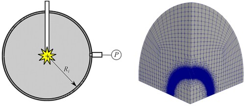
In order to validate the CFD model, simulation of the combustion sequence with different physical models was benchmarked against the time evolution of experimental variables, such as pressure, with the predictions provided from numerical simulations. The mesh used for simulation is represented in Figure 1 (Right).

Figure 1. (Left) Simplified geometry of the spherical bomb estimated for the modeling of this test and (Right) detail of the computational grid with a refinement strategy near the flame front.

As for the modeling of the ignition sequence, in the case of spark type, it is a common practice to follow the approach described by Liberman et al. (2011). It considers that the beginning of the initiation sequence can be modeled as an isobaric, quasi-instantaneous, heating process, that affects a very small volume of the domain (i.e. the ignition volume). In this work, different enthalpies and radius of ignition were tested (all for spherical volumes). An increase of the gas enthalpy within the ignition volume, corresponding to an energy spark around 800 kJ/m^3, was enough to make progress the laminar autoignition sequence.

3.1.1. Influence of the spatial discretization strategy

In order to evaluate the influence of the spatial grid resolution on the model results, it was performed an analysis of the influence of the grid size on the flame front and the reacting layer. Table 2 summarizes the results of the convergence analysis compared with experimental data from Goulier, Comandini, et al. (2017), for similar H₂/Air composition and conditions than in the H-EXP1 case. These values were calculated from the flame properties obtained for the different 3D computational grids tested with no sub-grid modeling (hereafter called laminar case). Results showed that the unstretched laminar flame speed predicted with these models with meshes ${\delta }_L^0/\mathrm{\Delta }x$ ∼1 provided errors below 18%. However, when a mesh with ${\delta }_L^0/\mathrm{\Delta }x$ = 8 was used, the errors in the prediction of the unstretched laminar flame speed were smaller than 1%.

Table 2. Grid convergence analysis.

Case	$S_L^0(\mathrm{m}/\mathrm{s})$	${\delta }_L^0(|\mathrm{\nabla }T|\text{based})(\text{mm})$
Experimental Goulier, Chaumeix, et al. (2017)	0.92 m/s ($S_{Lref}$)	0.382 mm (${\delta }_{Lref}$)
CASE 1 (30° × 30°, ${\delta }_L^0/\mathrm{\Delta }x=0.5$ static mesh)	1.18 m/s (1.28·$S_{Lref}$)	1.734 mm (4.54·${\delta }_{Lref}$)
CASE 2 (30° × 30°, ${\delta }_L^0/\mathrm{\Delta }x=1$ static mesh)	1.09 m/s (1.18·$S_{Lref}$)	1.165 mm (3.05·${\delta }_{Lref}$)
CASE 3 (30° × 30°, ${\delta }_L^0/\mathrm{\Delta }x=4$ static mesh)	0.961 m/s (1.04·$S_{Lref}$)	1.090 mm (2.85·${\delta }_{Lref}$)
CASE 4 (1/8 Sphere, ${\delta }_L^0/\mathrm{\Delta }x=0.5$ dynamic mesh)	1.03 m/s (1.11·$S_{Lref}$)	2.049 mm (5.36·${\delta }_{Lref}$)
CASE 5 (1/8 Sphere, ${\delta }_L^0/\mathrm{\Delta }x=1$ dynamic mesh)	0.981 m/s (1.06·$S_{Lref}$)	1.117 mm (2.93·${\delta }_{Lref}$)
CASE 6 (1/8 Sphere, ${\delta }_L^0/\mathrm{\Delta }x=4$ dynamic mesh)	0.951 m/s (1.03·$S_{Lref}$)	0.769 mm (2.01·${\delta }_{Lref}$)
CASE 7 (1/8 Sphere, ${\delta }_L^0/\mathrm{\Delta }x=8$ dynamic mesh)	0.911 m/s (0.99·$S_{Lref}$)	0.394 mm (1.03·${\delta }_{Lref}$)

At the initial stage of the propagation, the fundamental unstretched laminar flame speed ($S_L^0$) was calculated from the spatial flame velocity (denoted as burning speed, $V_L^0$), and the expansion ratio at null strain (${\rho }_u/{\rho }_b$), as $S_L^0=\frac{{\rho }_b}{{\rho }_u}{V}_L^0$ (Giannakopoulos et al., 2015). This way, the effect of the different discretizations on obtaining a good prediction of the laminar flame with the detailed chemical kinetics was assessed. This analysis was performed using the 21-reactions model proposed by Williams in conjunction with the ISAT procedure. As shown in Table 2, coarse grids were not able to predict neither the unstretched laminar flame speed $S_L^0$ (cases 1, 2, and 4), nor the laminar flame thickness based on thermal gradient ${\delta }_L^0$ = (T_b–T_u)/max|$\mathrm{\nabla }T$| (cases 1–6). It was needed a ${\delta }_L^0/\mathrm{\Delta }x>6$ grid to obtain a realistic laminar flame (case 7).

Figure 2 (Left) shows the distribution of the main flame physical properties obtained in the laminar cases, plotted along a radius line, after 2 ms from the beginning of the sequence (flame spherical equivalent radius of 15 mm). Figure 2 (Right) represents three snapshots with different grids used for the resolution of the combustion region: 30° × 30° (case 4), and a 90° × 90° (cases 6, and 7). These cases were simulated using the k_sgs model and the 21-reactions model proposed by Williams and ISAT strategy. As shown, at the moment of the snapshot, when the spherical equivalent radius was approximately 26 mm, the flame surface was not completely spherical.

Figure 2. (Left) Distribution of main physical properties vs. distance from the center (‘Radius’), 2 ms after the ignition sequence (laminar cases). (Right) Details of different grids and refinement levels used for the resolution of the combustion region at 4 ms (flame surface with cells), with k_sgs model, CASE 4 (Top), CASE 6 (Center), and CASE 7 (Bottom).

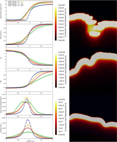
Regarding the performance of the meshing strategy, the grids of a spherical sector have the benefit of a smaller computational domain, and consequently, fewer cells for a given resolution. On other hand, with this kind of meshes, the cells aspect-ratio increased with the distance to the domain center, which is not recommended (Figure 2 Top-right). This might eventually break artificially the continuity of the flame, and might result in unphysical flame shape for low grid resolution (Case 4). However, with adequate grid resolution within the region with dynamic refinement, this potential problem disappeared. Therefore, Case 7 was the most appropriate to properly simulate the flame expansion (Figure 2 Bottom-right). On the other hand, results also showed that, in the case of considering a static mesh, the number of elements required to resolve the flame was higher than the one needed with the dynamic strategy. Due to this reason, to achieve that spatial resolution with affordable meshes, it was decided to use the dynamic mesh refinement process.

Figure 3 shows the numerical results of burning speed, defined as $\frac{\text{d}{r}_{eq}}{\text{d}t}$, where $r_{eq}$ is the spherical equivalent radius, computed as $r_{eq}={\left(\frac{3}{4}\cdot V_{burnt}/\pi \right)}^{1/3}$, with $V_{burnt}$ the total volume of the burnt region. Results show that, despite the difference in the flame thickness provided by meshes with ${\delta }_L^0/\mathrm{\Delta }x=4$ (cases 3 and 6), it is possible to achieve a reasonably good prediction, in terms of burning speed, for the model considered. It is worth mentioning the similarities in the burning speed obtained especially in cases 6 and 7, which predict the flame burning speed properly with LES and detailed chemistry.

Figure 3. Flame burning speed versus spherical equivalent radius for different meshes.

Results in Figure 3 suggest that the model proposed is able to predict the burning speed at the beginning of the combustion sequence (i.e. initiation and initial flame acceleration), when the Reynolds number is low. Regarding the validity of the LES approach, it was confirmed to be directly related to the mesh resolution (filter size $\mathrm{\Delta }$), as well as to the intensity of the sub-grid mixing. In order to assess the validity of this assumption for the different computational grids, the regime diagram proposed by Pitsch (2006) was employed. This diagram was designed for premixed combustion in LES using the filter size $\mathrm{\Delta }$ as the length scale and the subfilter velocity fluctuations $u_{\mathrm{\Delta }}^{\mathrm{\prime }}$ as the velocity scale. This takes into account not only physical properties of the combustion regime, but also modeling parameters, since the effect of the filter size is included. The parameters relevant in this diagram are the sub-grid Reynolds $(R{e}_{})$, sub-grid Damköhler $(D{a}_{})$ and the Karlovitz $(Ka)$ numbers, defined as (Pitsch, 2006): (14) $R{e}_{}=\frac{\text{u}{{}^{\mathrm{\prime }}}_{}}{s_L{l}_F}$(14) (15) $D{a}_{}=\frac{s_L}{\text{u}{{}^{\mathrm{\prime }}}_{}{l}_F}$(15) (16) $Ka=\sqrt{\frac{\text{u}{{{}^{\mathrm{\prime }}}_{}}^3{l}_F}{{s_L}^3}}$(16)

Figure 4 shows the evolution of these parameters obtained for cases 3, 5, 6 and 7. These values were sampled over the flame surface and averaged in each time step. Using the relationship $\mathrm{\Delta }/{\delta }_L$ and the $Ka$ values obtained during the complete combustion sequence, one may obtain the zone regions of each case within the regime diagram, as shown in Figure 5.

Figure 4. Evolution of nondimensional modeling parameters for different computational grids. (Left) $\mathit{R}{\mathit{e}}_{\mathrm{\Delta }}$ (Center) Karlovitz and (Right) $\mathit{D}{\mathit{a}}_{\mathrm{\Delta }}$

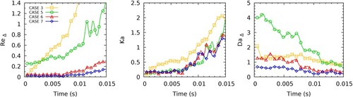
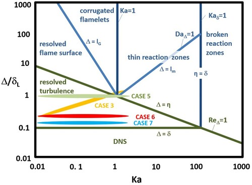
Figure 5. Regime diagram proposed by Pitsch (2006) with the points obtained for cases 3, 5, 6, and 7.

The validity of the perfectly stirred reactor hypothesis can be addressed by the level of the sub-grid mixing intensity at the given length scale $\mathrm{\Delta }$. In order to fulfill this hypothesis, the sub-grid mixing effects must act faster than any chemical reaction. This implies that the sub-grid structure characteristic time scale ${\tau }_{\mathrm{\Delta }}\sim \mathrm{\Delta }/u_{\mathrm{\Delta }}^{\mathrm{\prime }}$ must be smaller than the chemical time scale ${\tau }_c\sim {\delta }_L/S_L$. This leads to $D{a}_{}<1$ as a requirement for the validity of the perfectly stirred reactor assumption in the cases where the flow conditions are not laminar, or the mesh resolution is far from the grids required for DNS. As shown in Figure 4 (Right), when the mesh size is smaller, and consequently $\mathrm{\Delta }$ decreases, $D{a}_{}$ values also decreases.

The combustion experiments used in the present work (Goulier, Comandini, et al., 2017; Sabard et al., 2013), were carried out in initial calm conditions (i.e. with no flow velocity within the scenario) where low $R{e}_{\mathrm{\Delta }}$ and $K{a}_{\mathrm{\Delta }}$ values are expected. That means that a small filter size would be needed to ensure well-stirred sub-grid concentrations and temperatures. This is only achieved in case 7, according to the $D{a}_{}$ values reported in Figure 4. In addition, the low $Ka$ values reported (especially for the cases 5, 6, and 7) indicate that the sub-grid modeling does not alter the flame structure, being the chemical region in laminar conditions, where the perfectly stirred reactor assumption is valid. As shown in Figure 4 (Left), the sub-grid turbulent intensity increases with the propagation of the flame, due to the flow velocity fluctuations induced by the propagation of the flame front. As a consequence, the Karlovitz values increase, reducing the $D{a}_{}$ values in the reacting zone. This relaxes the mesh cell size requirement, which permits case 6 to fulfill the $D{a}_{}<1$ criterium, at $t=6$ ms. As shown in Figure 5, all points in simulations fall within the region of resolved turbulence for the cases 6 and 7, which may indicate that, in practice, the turbulence-chemistry interactions may be well simulated at grid-scale level. In fact, the burning speeds predicted in the four cases represented in Figure 5 were quite accurate, as shown in Figure 3.

In this section, the validity of the model at the initial stages of the combustion sequence was assessed. For the simulations presented in the next sections, case 7 with dynamic mesh refinement is the selected strategy.

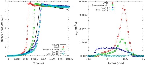
3.1.3. Influence of the sub-grid scale turbulence model

In order to analyze the influence of the LES model used, the experimental data previously commented (Sabard et al., 2012; Sabard et al., 2013) is used. The influence of the sub-grid scale turbulence model used will be assessed, based on the experimental benchmark H-EXP1. For these conditions, Figure 6 (Left) shows pressure evolution as a function of time. The figure also includes the experimental data recorded at the wall of the sphere during the experiment. Different LES sub-grid scale models are applied, together with the chemical model by Williams and ISAT tabulation: Smagorinsky-Lilly, WALE, k_sgs-equation, and Dynamic Anisotropic k_sgs-equation. These models provide different results in the prediction of the pressure history at the wall of the sphere (Figure 6 (Left)). k_sgs-equation model provides the best prediction compared to the experimental data. The Smagorinsky-Lilly model shows less stable behavior, when the flame front is close to the wall. With this model, the flame accelerates at a higher rate, getting the wall faster than in the case of the k_sgs-equation model. As shown, the WALE model also overestimates the flame acceleration. The reasons behind this dissimilar behavior partially rely on the different estimation of the transport phenomena (sub-grid scale viscous term, ${\nu }_{\text{sgs}}$) provided by each model. Figure 6 (Right) permits to illustrate this point. The figure presents the spatial distribution of the sub-grid viscous term provided by the four different models in the flame front region. The ${\nu }_{sgs}$ obtained by the dynamic k_sgs-equation model is negligible compared to the one obtained with the other sub-grid scale models within the flame front, whereas it is not null in front and behind the flame front region at 2·10⁻³ s of simulated time. Regarding the non-dynamic sub-grid models, the k_sgs-equation model estimated the smallest value for the sub-grid scale viscous term ${\nu }_{sgs}$ in the region of the flame front, although it reported higher values downstream flame front. On the other hand, WALE and Smagorinsky-Lilly models predicted higher values of the subgrid diffusive terms. These differences might also be explained by their different properties. WALE was tuned to predict the y⁺³ profile of the effective viscosity close to walls, under non-reacting flow conditions. However, the k_sgs-equation models are able to overcome the deficiency of local balance assumption between the sub-grid scale energy production and dissipation adopted in algebraic eddy viscosity models as the Smagorinsky-Lilly and WALE (Nicoud & Ducros, 1999). On the other hand, WALE and Smagorinsky-Lilly models were originally tuned against experimental data in incompressible conditions (Nicoud & Ducros, 1999), whereas k_sgs-equation models were designed for compressible flowconditions.

Figure 6. (Left) Influence of the LES modeling on the pressure evolution at sphere wall (H-EXP1 conditions). (Right) Different kinematic sub-grid scale viscosity values obtained in the frame front region with the tested LES models (t = 2·10⁻³s H-EXP1 conditions).

When comparing both versions of the k_sgs-equation model, the main difference is the ‘non-dynamic’ one (here denoted simply as k_sgs-equation model) slightly underestimates the pressure rise near the wall, upstream the flame front (in the time lapse rounding 15 ms). As a result, it overestimates the deflagration factor near the wall, which is proportional to $\text{d}P/\text{d}t$. All in all, Figure 6 shows an important effect of the sub-grid models what points out the uncertainty linked with its election. The differences found among the models might be due to the fact that sub-grid scale models are developed, case by case, based on operators originally designed to behave more ‘accurately’ when facing certain canonical problems such as homogeneous isotropic turbulent flow, pure shear flows, pure rotating flows or wall flows in turbulent channels. Some examples of this challenging developing process can be found in the works of Sankaran and Menon (2005), Lilly (1991), Wallin and Johansson (2000), Nicoud and Ducros (1999) and Yoshizawa and Horiuti (1985). Overall, in the case of unsteady combustion problems, such as the one presented here, it is of paramount importance to benchmark LES against experimental data to ensure reliable results.

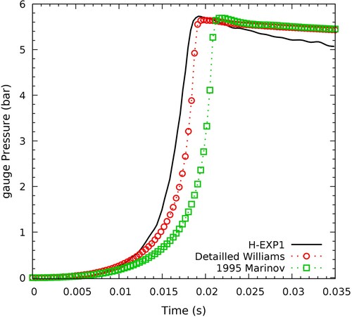
3.1.4. Influence of the chemical kinetics model

A comparison of the pressure evolution at the sphere predicted with two different chemical kinetic models is shown in Figure 7. These two are detailed chemical combustion models: the one by Williams (2008), and the one by Marinov et al. (1995). In both cases, ISAT tabulation was used to reduce the computational cost of the integration of these detailed models. The figure includes the experimental pressure recorded at the wall of the sphere during H-EXP-1. As shown, both detailed combustion models predict with reasonable accuracy the wall pressure evolution with time, with a slight delay in pressure rise for both models. Nonetheless, the model by Williams gives more accurate results. Altogether, the comparison permits to estimate the uncertainty linked to the use of different detailed chemical kinetic models. As shown, results were less sensitive to the detailed kinetic model than to the LES sub-grid scale model.

Figure 7. Influence of hydrogen combustion modeling on the pressure evolution at sphere wall (H-EXP1 conditions).

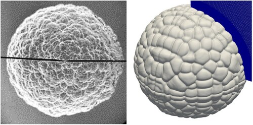
3.1.5. Cellular flames pattern

In the configuration studied in this work, the flame is initially laminar. During the initial stages of the flame expansion, the flame thickness is enough to permit this LES approach to resolve with a reasonable agreement the reacting flow phenomena. Under these lean H₂/O₂ conditions, thermodiffusive instabilities should occur leading to the formation of cellular flames. As previously said, the model considers an effective Lewis number equal for all species, and smaller than unity. Its value can be obtained from experiments (Goulier, Comandini, et al., 2017). Under these conditions, the simulation performed with detailed chemistry models, and with enough mesh resolution to resolve the flame front, should account for these instabilities, and the strain effects of the flame should be taken into account intrinsically with the model used. Figure 8 shows a comparison of the flame pattern observed in the experiments of Goulier, Comandini, et al. (2017), and the simulated pattern obtained for the same conditions. The numerical flame surface is represented as an isosurface based on a variable which represents a numerical Schlieren (based on the normalized density gradient). As shown in Figure 8, the numerical approach is able to account for this flame pattern, and provides results qualitatively similar to the experimental ones. Also, the critical radius at which the cellular cell pattern appears is predicted to be around 20 mm for an H₂-Air mixture of 20%, which is in agreement with the experimental measurements of Goulier, Comandini, et al. (2017).

Figure 8. Experimental flame with 60 mm of equivalent radius from Goulier, Comandini, et al. (2017) (Left), and numerical results of the present work (Right), representing the flame pattern for 20% molar fraction of H₂/air at 60 mm of equivalent radius.

3.1.6. Experimental benchmark and assessment of numerical schemes

In this section, the numerical schemes presented in Section 2.4 are analyzed by benchmarking against experimental data. Tables 3 and 4 show numerical predictions in terms of maximum wall pressure and sequence time, for the different numerical schemes considered. Regarding the estimation of maximum combustion pressure ($P_{max}$), the use of the different approaches entails less than 4% of error, except for Rusanov's scheme. As for the prediction of the combustion time ($t_{rise}$), PISO, AUSMup and AUSM+ showed better prediction capacities. This is somehow expected, as the Rusanov scheme is known to be very diffusive, and it is not accurate for low Mach flow conditions, whereas AUSM is very efficient in transonic conditions (Prá et al., 2010; Velasco et al., 2016), and its variations (AUSM+, and AUSMup) are also adequate for a wide range of Mach values (Liou, 1996,2006).

Table 3. Model predictions of maximum pressure and pressure rise time. H-EXP1.

H-EXP1	Experimental	PISO	AUSMup (Barth-Jespersen)	AUSM+ (Barth-Jespersen)	RUSANOV (Barth-Jespersen)
Pmax (bar)	5.72	5.68	5.74	5.74	7.14
Error Pmax (%)	Ref.	0.67	0.31	0.37	24.84
trise (ms)	19.20	19.74	19.49	18.44	5.12
Error trise (%)	Ref.	2.81	1.51	−3.96	−73.33
H-EXP1	AUSMup (Van-Leer)	AUSMup (Van-Leer) (Runge Kutta)	AUSMup (MUSCL)	AUSMup (Van-Albada)	AUSMup (Upwind)	AUSM+ (Van-Leer)
Pmax (bar)	5.67	5.66	5.72	5.65	5.65	5.65
Error Pmax (%)	−0.86	−1.14	0.077	−1.15	−1.22	−1.20
trise (ms)	21.66	20.15	16.54	21.66	16.15	20.26
Error trise (%)	12.81	4.95	−13.85	12.81	−15.89	5.52

Table 4. Model predictions of maximum pressure and pressure rise time (H-EXP2).

H-EXP2	Experimental	PISO	AUSMup (Barth-Jespersen)	AUSM+ (Barth-Jespersen)	AUSMup (Van-Leer)	AUSMup (Van-Leer) (Runge Kutta)	AUSM+ (Van-Leer)
Pmax (bar)	5.585	5.663	5.712	5.694	5.638	5.62	5.616
Error Pmax (%)	Ref.	1.41	2.28	1.94	0.94	0.65	0.55
trise (ms)	16.20	16.98	16.13	15.3	18.98	17.12	17.88
Error trise (%)	Ref.	1.28	−6.22	−11.05	10.35	−0.47	3.95

Regarding the prediction of the unsteady behavior of the sequence, Figures 9 and 11 show the wall pressure evolution predicted by the different schemes. In general, most of the numerical approaches capture the evolution, although with different precision. Flux difference splitting schemes (FDS), as Rusanov’s, show a too diffusive behavior. Figure 10 permits to support this point. In this figure, it is represented the radial distribution of the net mass flux in each cell in the surroundings of the flame front. As shown, Rusanov scheme predicts a wider spatial region of positive cell net mass flux, compared to the AUSM-type schemes for the same primitive spatial interpolation scheme used in the cell-to-face reconstruction. As a result, the flame thickness numerically obtained with this scheme is also larger (Figure 11, Right), what increases the heat released due to combustion, and provides a non-realistic burning speed. As a result, the scheme does not provide a realistic dynamic of the combustion sequence.

Figure 9. Influence of the numerical scheme. Time evolution of gauge pressure at the sphere wall (H-EXP1 conditions).

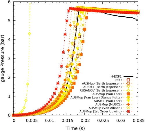
Figure 10. Cell net mass fluxes in the flame front region at 10⁻³ s after initiation sequence (H-EXP1 conditions).

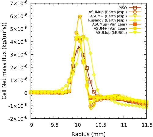
Figure 11. Numerical and experimental results of gauge pressure at the sphere wall (H-EXP2 conditions).

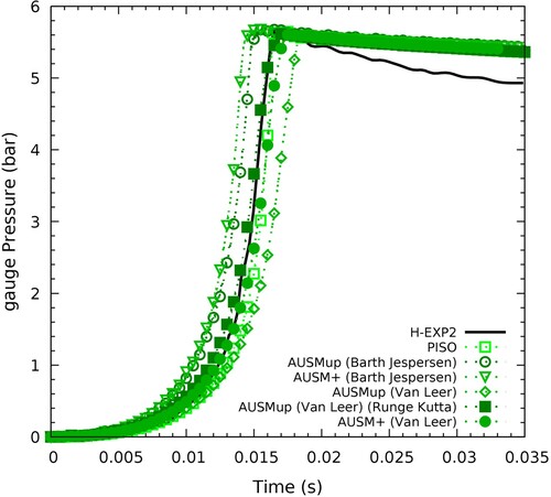
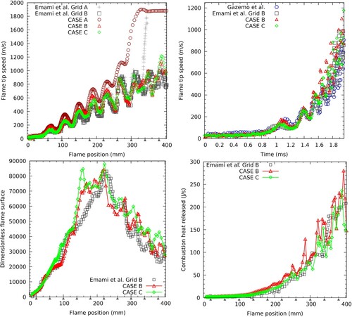
Figure 12. Comparison of the results predicted in the present work against the numerical prediction by Emami et al. (2015) and Gamezo et al. (2007). Top-left: Flame tip speed versus flame position. Top-right: Flame tip speed versus simulated time. Bottom-left: Dimensionless flame surface area versus flame position. Bottom-right: Flame heat released versus flame position.

On the other hand, a coupled solver with flux vector splitting (FVS) schemes, such as AUSMup and AUSM+ can provide better results under the conditions of the experiment. In this case, AUSMup flux-schemes, with the Bath-Jespersen slope limiter, provide the best results, not only in maximum pressure at the wall but also in the rising time predicted. These schemes are less diffusive and do not introduce artificial numerical transport of the conserved variables, resulting in a thinner flame front with a more accurate combustion heat release. PISO segregated solver shows stability and robustness under the subsonic conditions of the experiments. It also provides a reasonable agreement on the dynamic evolution of wall pressure at the late stage of the sequence.

As shown in Figure 11, the effect of increasing the oxygen fraction in the gas mixture (as defined for H-EXP2) is well captured by the numerical models, although different time evolutions are predicted, with errors between −0.4% and 11% in terms of rising time (t_rise), and between 0.5% and 1.4% in terms of peak pressure (P_max), as summarized in Table 4. PISO and AUSMup (Van-Leer, Runge–Kutta) are the schemes that provide the smallest prediction errors. AUSMup (Van-Leer, Runge–Kutta) scheme gives the best prediction of pressure evolution during the period when $\text{d}P/\text{d}t$ reached maximum values (i.e. during the intermediate lapse of time of the sequence, 11 < t < 17 ms), whereas PISO scheme yields a better prediction at low-pressure conditions (i.e. during the initial stage of the sequence t < 11 ms). All in all, PISO and AUSMup (Van-Leer, Runge–Kutta) provide the smallest averaged errors for both experiments.

Concerning the benchmark for the combustion products, Table 5 presents a comparison of the experimental data and the model predictions with different schemes and Williams chemical model. As shown, the models can predict the final composition, with errors smaller than 6%. PISO, with Williams’ chemical model, provides the smallest deviations from experimental data. Similar results are obtained with the same scheme and Marinov’s chemical model, although with slightly bigger errors.

Table 5. Benchmark of the combustion products with Williams (2008) and Marinov et al. (1995) chemistry models.

H-EXP1 (% mol)	EXPERIMENTAL	PISO (Williams ch.)	AUSMup BJ (Williams ch.)	AUSM+ BJ (Williams ch.)	AUSMup VL (Williams ch.)	PISO (Marinov ch.)
%H2	0.00	0.05	0.22	0.22	0.17	0.08
%H	0.00	0.01	0.22	0.05	0.04	0.01
%O2	7.65 ± 0.50	7.46	7.21	7.21	7.31	7.41
%O	0.00	0.04	0.17	0.17	0.14	0.06
%OH	0.00	0.40	1.14	1.14	0.98	0.58
%HO2	0.00	0.00	0.00	0.00	0.00	0.00
%H2O2	0.00	0.00	0.00	0.00	0.00	0.00
%H2O	22.59 ± 0.50	21.93	22.72	22.62	21.45	21.80
%N2	69.76 ± 0.50	70.11	68.47	68.58	69.91	70.06
Error (%)
%O2	–	2.50	5.73	5.71	4.44	3.13
%H2O	–	2.90	−0.60	−0.13	5.04	3.50
%N2	–	−0.50	1.85	1.69	−0.22	−0.43
H-EXP2 (% mol)	EXPERIMENTAL	PISO (Williams ch.)	AUSMup BJ (Williams ch.)	AUSM+ BJ (Williams ch.)	AUSMup VL (Williams ch.)
%H2	0.00	0.03	0.01	0.01	0.01
%H	0.00	0.01	0.00	0.00	0.00
%O2	14.68 ± 0.50	15.44	15.42	15.44	15.50
%O	0.00	0.05	0.02	0.02	0.02
%OH	0.00	0.44	0.25	0.25	0.25
%HO2	0.00	0.00	0.00	0.00	0.00
%H2O2	0.00	0.00	0.00	0.00	0.00
%H2O	22.82 ± 0.50	21.93	22.28	22.23	22.07
%N2	62.5 ± 0.50	62.10	62.02	62.05	62.15
Error (%)
%O2	–	−5.16	−5.04	−5.19	−5.62
%H2O	–	3.90	2.37	2.59	3.29
%N2	–	0.64	0.78	0.73	0.56

3.2. Flame acceleration in an obstructed channel

In order to assess the capability of this combustion modeling strategy to predict flame acceleration phenomena of H₂-Air mixtures, simulations in an obstructed channel were carried out. The results presented in this section show the capabilities of ILES for this purpose, with different modeling procedures, taking into account its behavior under flame-vortex interactions. The simulation conditions are set to reach the turbulent combustion regime during the sequence. That allows us to extend the evaluation of this modeling approach as a potential global strategy that might permit to simulate a complete combustion sequence, from the initial stages (laminar) to the fully turbulent combustion regime.

A 2D channel, 4 cm wide and 64 cm long, with a blockage ratio of 0.5 is considered for this study. It is filled in with rectangular obstacles of width $d/16$, and length $d/4$, being $d$ the channel width. The obstacles are equally spaced along the channel. The distance between two consecutive obstacles is set to $d$. The first obstacle is placed at a longitudinal distance of $d/2$ from the ignition side. Simulations on a similar channel were carried out by Gamezo et al. (2007) for a stoichiometric H₂-Air mixture, and initial conditions of 1 atm and 293 K. These conditions result in flame laminar properties of $S_L^0=2.98\text{ m}/\text{s }$ and ${\delta }_L^0=0.35\text{mm}$, as reported by Gamezo et al. (2007).These computations were performed with a Godunov-type solver with no turbulence, in conjunction with a one-step Arrhenius kinetic model. A more recent study was performed by Emami et al. (2015) using a PISO solver with the 27-steps Marinov’s chemical mechanism, ISAT tabulation, and the k_sgs modeling, as performed in this work, but with the difference of using an Artificially Thickened Flame (ATF) for the modeling of the sub-grid scale combustion effects. In that case, cell sizes of 0.125 and 0.0625 mm were employed. More detailed information about the channel geometry and physical properties of the flame can be found in Gamezo et al. (2007).

In the present work, computational domains with a discretization of 0.0875 mm (${\delta }_L^0/\mathrm{\Delta }x=4$) and 0.04375 mm (${\delta }_L^0/\mathrm{\Delta }x=8$) are used, to keep a similar grid resolution to that analyzed in the deflagration validation in section 3.1.1. Also, the PISO algorithm and an ignition volume with 5 mm of radius are considered. The same algorithm and ignition volume were used by Emami et al. (2015). No-slip boundary conditions are imposed at the wall surfaces. The channel is opened at its end, where a wave-transmissive boundary condition is imposed. A symmetry plane is imposed at the horizontal midplane of the channel (upper horizontal boundary in Figure 13) so that the computational domain considered is half of the channel. In order to perform the LES simulations on the 2D domain correctly, a structured mesh with a uniform cell size is considered, where the cell size ($\mathrm{\Delta }x$) is the third cell dimension (i.e. 3D domain with an extrusion length of $\mathrm{\Delta }x$ in the third spatial direction, not resolving velocities and gradients in this direction). This way, the filter size for the LES sub-grid scale modelization is properly calculated from the cell volume. Besides, an effective Lewis of unity is considered. This is approximately the value reported by Goulier, Chaumeix, et al. (2017), for a stoichiometric H2-Air mixture under similar conditions.

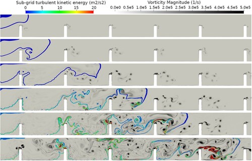
Figure 13. Vorticity field with the flame front colourized by sub-grid turbulent intensity during the flame acceleration sequence between obstacles 1 and 6 (CASE B). From top to bottom: 0.9, 1.4, 1.8, 2.0, 2.1 and 2.2 ms of simulated time.

Three different simulations are presented: two of them with the 21-step chemical mechanism by Williams, one with ${\delta }_L^0/\mathrm{\Delta }x=4$ (CASE A) and another with ${\delta }_L^0/\mathrm{\Delta }x=8$ (CASE B); finally, a third one with ${\delta }_L^0/\mathrm{\Delta }x=8$ and the 27-step chemical mechanism by Marinov (CASE C), to assess the influence of the chemical mechanism in the computations. Note that ISAT method is used. This strategy was also adopted by Emami et al. (2015).

Figure 12 shows a comparison of the results predicted with the present approach against the numerical prediction by Emami et al. (2015) and Gamezo et al. (2007). The images at the top illustrate the flame tip speed versus the flame position and time, whereas the images at the bottom represent the dimensionless flame surface area versus flame position, as well as the combustion heat released versus the flame position. Note that the ordinate axes include both the position of the obstacles and the flame. The flame position was computed as the largest distance of the flame surface from the ignition point, whereas the flame surface was defined as the isosurface where ${\text{Y}}_{\text{H}2}=0.5\cdot {\text{Y}}_{\text{H}2}^0$. Here, ${\text{Y}}_{\text{H}2}^0$ denotes the initial H₂ mass fraction of the premixed mixture within the channel. As shown, the present ILES approach can describe the flame acceleration mechanism in good agreement with the approaches used by Emami et al. and Gamezo et al. It is worth to be noted that the results of Figure 12 (Top-left) were shifted by 0.65 ms for a better comparison of the results by Emami et al. (2015) against those by Gamezo et al. (2007). Emami et al. attributed this time difference to the different chemical induction times obtained with the one-step mechanism used by Gazemo et al. compared to the detailed Marinov’s mechanism used by Emami et al. This induction time was reported by the authors to be a few times smaller for a one-step mechanism, when compared to real induction times (Liberman et al., 2010).

Concerning the results of the present work, they were also shifted by 0.65 ms for CASE C (Marinov’s mechanism) but only 0.5 ms for CASE B (Williams’ mechanism). This shifting revealed that, during the initial stage of the propagation, where the flame is laminar, the chemical mechanism and the modelization of the heat capacities of the mixture are key aspects to predict accurately the burning flame speed. Note that the values reported by Emami et al. with an ATF combustion modeling and those reported in this work were shifted by the same value when considering the same reaction mechanism. This confirmed the agreement of the present approach with the one of Emami et al. [61]. In addition, the comparison of CASE A and B show that the grid-independent solution found for the initial stage of the flame acceleration (Figure 12 Top-Left) is lost at a later stage of flame acceleration, when the coarse mesh (CASE A) is not able to follow the tendency of the refined one (CASE B). Notwithstanding, CASE B ($\frac{{\delta }_L^0}{\mathrm{\Delta }x}=8$) provides a reasonably good prediction of the numerical results in Gamezo et al. (2007) and Emami et al. (2015), for a turbulent flow regime with medium-high Reynolds numbers.

Figures 13 and 14 show some 2D snapshots of the sequence and permit to get some insights into the acceleration mechanism. Figure 13 shows the vorticity field with colourized flame front during the flame acceleration between obstacles 1 and 6 (CASE B), whereas Figure 14 shows a numerical Schlieren with the flame front colourized by H₂ reaction rate during the sequence. In these figures, the flame front is represented as an isovolume with H₂ mass fraction values between 0.5 and 23%.

Figure 14. Numerical Schlieren with the flame front colourized by H₂ reaction rate during the flame acceleration sequence between obstacles 1 and 6 (CASE B). From top to bottom: 0.9, 1.4, 1.8, 2.0, 2.1 and 2.2 ms of simulated time.

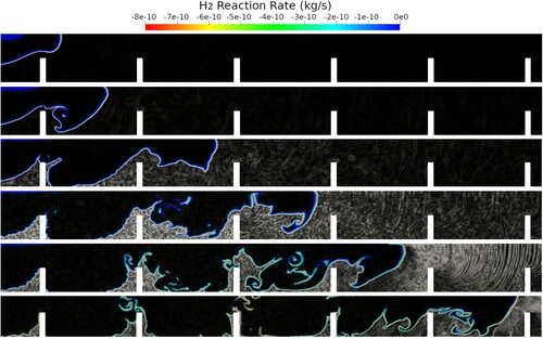
As shown in Figures 12–14, the flame progressively accelerates as it surpasses the subsequent obstacles. At the initial stage, this acceleration is promoted by the increase of the effective flame surface area during the flame expansion (Figure 12 Top-Left). As the flame front surpasses an obstacle, the vortex shedding process increases the effective area of the flame (Figure 13). Once the flame surface area reaches its maximum value (Figure 12 Bottom-Left and Figure 13, obstacles 4-6), the promotion of the flame acceleration is mainly sustained by the combustion heat released, increased with the turbulence enhancement (Figure 14). Figures 13 and 14 also permit to show the interaction of the vortex and flame front during the flame acceleration. As the flame accelerates, the compressibility effects become significant, and the vortex structures induce the deformation of the flame front, increasing not only turbulence features but also local precursors of ‘hot-spots’. The presence of the obstacles also promotes the reflection of the local density gradient waves, which also distort the flame front, increasing its area and promoting the transition of the flame combustionregime.

4. Major limitations and needs of the model

The benchmarks performed permit to identify several shortcomings of this LES approach, that should be considered and addressed. These can be summarized as follows:

• Results show that the unstretched laminar flame speed predicted with this type of models with meshes ${\delta }_L^0/\mathrm{\Delta }x$ ∼1, provide errors of ∼18%. In this case, the numerical diffusion (i.e. numerical errors) might play an important role in the predicted flame speed.

• There is an important effect of the sub-grid models, which points out the uncertainty linked with its election, especially in the case of grids that do not provide enough flame resolution.

• In practice, the present LES approach can be only used in the initial stages of unsteady combustion sequences, due to computational cost, as the grid conditions required in the absence of sub-grid combustion modeling are difficult to satisfy when the flame surface increases.

• This study has pointed out some uncertainties and grid resolution requirements that must be controlled rigorously, to provide reliable results. Therefore, the present LES approach is not recommended or, at least, should be used with great care, if applied to critical applications. In those applications, other LES approaches, such as TFM / ATF (Nicolás-Pérez et al., 2020), would permit to relax those criteria.

The analysis of these limitations has highlighted major requirements or needs that must be fulfilled to use this LES approach under unsteady sequences. Among them, the grid resolution criterium was found to be critical. For the specific conditions of the cases considered in this work, at least ${\delta }_L^0/\mathrm{\Delta }x$ ∼8, and $D{a}_{}<1$ should be respected. However, these criteria should be checked for other types of configurations.

5. Conclusions and future work

In this study, the capabilities and limitations of LES coupled with the PSR hypothesis were evaluated to simulate the initial stages of H₂-air combustion experiments. This approach considers that there is a homogeneous concentration and temperature in each computational cell at sub-grid level. Different sub-grid turbulence and detailed chemistry models were tested in both experimental and numerical benchmarks. This permitted to evaluate the capabilities and limitations of this modeling approach when simulating unsteady combustion sequences with low or moderate Reynolds numbers. The study showed this LES approach can be applied to a grid with enough resolution to resolve flame thickness and wrinkling patterns. In this case, no sub-grid scale combustion modeling is needed. However, the model has important limitations that must be considered:

• Spatial resolution was found to be critical. The unstretched laminar flame speed predicted with this type of models with meshes ${\delta }_L^0/\mathrm{\Delta }x$ ∼1 provide errors of ∼18%. Furthermore, numerical diffusion might play an important role in the predicted flame speed.

• There is an important effect of the sub-grid models, which points out the uncertainty linked with its election, especially in the case of grids that do not provide enough flame resolution.

• The computational resources needed to reach the required level of flame resolution of this modeling approach increases as the flame expands and the flow increases its Reynolds number due to flame wrinkling and the effective increase of the flame surface.

As for the suggested improvements, results also showed this LES approach coupled with detailed chemistry and ISAT method was an affordable strategy to simulate the initial stages (i.e. post-ignition and flame acceleration) of premixed combustion problems, with low or moderate Reynolds numbers with reasonable accuracy, if a certain level of grid refinement was reached (${\delta }_L^0/\mathrm{\Delta }x\ge 8$).

Besides, the benchmarks highlighted other significant specifics:

• The impact of sub-grid turbulence models was found to be high whereas the influence of the detailed kinetic scheme used was lower. Therefore, it is recommended to benchmark the sub-grid model used against experimental results.

• Regarding the prediction of the unsteady behavior of the sequence, AUSMup, AUSM+, and PISO schemes showed reasonable agreement with experimental data. Flux difference splitting (FDS) schemes as Rusanov scheme showed not accurate performance at low Mach regime. AUSMup flux-schemes with the Bath-Jespersen slope limiter provided the best results (<4% of error), not only in rising time but also in maximum wall pressure predicted.

• As for the prediction of the combustion products, the models predicted, with an error smaller than 6%, the final species composition. PISO scheme and Williams’ chemical model provided the smallest deviations from experimental data.

Finally, the results also showed that this LES approach was able to account for the cellular flame pattern at the post-ignition phase, and provided results which were qualitatively similar to the experimental ones. Besides, this approach is also able to predict flame acceleration in an obstructed channel if the required level of flame resolution is met. These results permit to postulate this LES approach for experiments interpretation and dynamic studies of the early stage of a flame expansion.

The study also permits to identify research needs that should be addressed to improve the reliability of this LES approach. In this sense, the future direction of this work will focus on the extension of the benchmark of this LES approach with others based on reference experimental or numerical data to assess its limitations in different key combustion problems. Additional efforts should be also devoted to the development of combustion and sub-grid turbulence models or strategies with lower computational costs which could be applied to the simulation of transient combustion sequences.

Disclosure statement

No potential conflict of interest was reported by the author(s).

Additional information

Funding

This work was performed with the support of Institut of Radioprotection et Sûreté Nucléaire of France [DA 3000011012/CA32000911] IRSN SIRET: 440 546 018 00019 Code APE: 7219 Z and with resources of Servicio de Apoyo a la Investigación Tecnologlócia of UPCT which was supported by the Spanish Ministry of Economy and Competitiveness and the European Commission (European Regional Development Fund ERDF) [UPCA13-2E-2352].

References

- Agilent Corp. (1994). Agilent chemical analysis group 5890 gas chromatograph. 5890 Series II. http://www.agilent.com/cs/library/support/documents/a15282.pdf.
- Barth, T. J., & Jespersen, D. C. (1989). The design and application of upwind schemes on unstructured meshes. AIAA Journal, 0366. https://doi.org/https://doi.org/10.2514/6.1989-366
- Berglund, M., Fedina, E., Tegnér, J., Fureby, C., & Sabelnikov, V. (2010). Finite rate chemistry LES of self-ignition in a supersonic combustion ramjet. AIAA Journal, 48(3), 540. https://doi.org/https://doi.org/10.2514/1.43746
- Chai, X., & Mahesh, K. (2012). Dynamic k-equation model for Large Eddy Simulations of compressible flows. Journal of Fluid Mechanics, 699, 385–413. https://doi.org/https://doi.org/10.1017/jfm.2012.115
- Chen, C., Riley, J. J., & McMurtry, P. A. (1991). A study of Favre averaging in turbulent flows with chemical reaction. Combustion and Flame, 87(3–4), 257–277. https://doi.org/https://doi.org/10.1016/0010-2180(91)90112-O
- Ciccarelli, G., Johansen, C. T., & Parravani, M. (2010). The role of shock-flame interactions on flame acceleration in an obstacle laden channel. Combustion and Flame, 157(11), 2125–2136. https://doi.org/https://doi.org/10.1016/j.combustflame.2010.05.003
- Colin, O., Ducros, F., Veynante, D., & Poinsot, T. (2000). A thickened flame model for Large Eddy Simulations of turbulent premixed combustion. Physics of Fluids, 12(7), 1843–1863. https://doi.org/https://doi.org/10.1063/1.870436
- Dodoulas, I. A., & Navarro-Martinez, S. (2013). Large Eddy Simulation of premixed turbulent flames using the probability density function approach. Flow, Turbulence and Combustion, 90(3), 645–678. https://doi.org/https://doi.org/10.1007/s10494-013-9446-z
- Duwig, C., Ducruix, S., & Veynante, D. (2012). Studying the stabilization dynamics of swirling partially premixed flames by proper orthogonal decomposition. Journal of Engineering for Gas Turbines and Power, 134(10), 101501. https://doi.org/https://doi.org/10.1115/1.4007013
- Duwig, C., & Dunn, M. J. (2013). Large Eddy Simulation of a premixed jet flame stabilized by a vitiated co-flow: Evaluation of auto-ignition tabulated chemistry. Combustion and Flame, 160(12), 2879–2895. https://doi.org/https://doi.org/10.1016/j.combustflame.2013.06.011
- Duwig, C., & Ludiciani, P. (2014). Large Eddy Simulation of turbulent combustion in a stagnation point reverse flow combustor using detailed chemistry. Fuel, 123, 256–273. https://doi.org/https://doi.org/10.1016/j.fuel.2014.01.072
- Duwig, C., Nogenmyr, K. J., Chan, C. K., & Dunn, M. J. (2011). Large Eddy Simulations of a piloted lean premix jet flame using finite-rate chemistry. Combustion Theory and Modelling, 15(4), 537–568. https://doi.org/https://doi.org/10.1080/13647830.2010.548531
- Emami, S., Mazaheri, K., Shamooni, A., & Mahmoudi, Y. (2015). LES of flame acceleration and DDT in hydrogen-air mixture using artificially thickened flame approach and detailed chemical kinetics. International Journal of Hydrogen Energy, 40(23), 7395–7408. https://doi.org/https://doi.org/10.1016/j.ijhydene.2015.03.165
- Fiorina, B., Mercier, R., Kuenne, G., Ketelheun, A., Avdic, A., Janicka, J., Geyer, D., Dreizler, A., Alenius, E., Duwig, C., Trisjono, P., Kleinheinz, K., Kang, S., Pitsch, H., Proch, F., Cavallo Marincola, F., & Kempf, A. (2015). Challenging modeling strategies for LES of non-adiabatic turbulent stratified combustion. Combustion and Flame, 162(11), 4264–4282. https://doi.org/https://doi.org/10.1016/j.combustflame.2015.07.036
- Fureby, C. (2007). Comparison of flamelet and finite rate chemistry LES for premixed turbulent combustion. 45th AIAA Aerospace Sciences Meeting and Exhibit Reno, Nevada. https://doi.org/https://doi.org/10.2514/6.2007-1413
- Gamezo, V. N., Ogawa, T., & Oran, E. S. (2007). Numerical simulations of flame propagation and DDT in obstructed channels filled with hydrogen–air mixture. Proceedings of the Combustion Institute, 31(2), 2463–2471. https://doi.org/https://doi.org/10.1016/j.proci.2006.07.220
- García-Cascales, J. R., Otón-Martínez, R. A., Velasco, F. J. S., Vera-García, F., Bentaib, A., & Meynet, N. (2014). Advances in the characterisation of reactive gas and solid mixtures under low pressure conditions. Computers & Fluids, 101, 64–87. https://doi.org/https://doi.org/10.1016/j.compfluid.2014.05.017
- Giacomazzi, E., Battaglia, V., & Bruno, C. (2004). The coupling of turbulence and chemistry in a premixed bluff-body flame as studied by LES. Combustion and Flame, 134(4), 320–335. https://doi.org/https://doi.org/10.1016/j.combustflame.2004.06.004
- Giannakopoulos, G. K., Matalon, M., Frouzakis, C. E., & Tomboulides, A. G. (2015). The curvature Markstein length and the definition of flame displacement speed for stationary spherical flames. Proceedings of the Combustion Institute, 35(1), 737–743. https://doi.org/https://doi.org/10.1016/j.proci.2014.07.049
- Goulier, J., Chaumeix, N., Halter, F., Meynet, N., & Bentaïb, A. (2017). Experimental study of laminar and turbulent flame speed of a spherical flame in a fan-stirred closed vessel for hydrogen safety application. Nuclear Engineering and Design, 312, 214–227. https://doi.org/https://doi.org/10.1016/j.nucengdes.2016.07.007
- Goulier, J., Comandini, A., Halter, F., & Chaumeix, N. (2017). Experimental study on turbulent expanding flames of lean hydrogen/air mixtures. Proceedings of the Combustion Institute, 36(2), 2823–2832. https://doi.org/https://doi.org/10.1016/j.proci.2016.06.074
- Grinstein, F. F., & Kailasanath, K. (1995). Three dimensional numerical simulations of unsteady reactive square jets. Combustion and Flame, 101(1–2), 2–10. https://doi.org/https://doi.org/10.1016/0010-2180(94)00095-A
- Hiremath, V., Ren, Z., & Pope, S. B. (2011). Combined dimension reduction and tabulation strategy using ISAT-RCCE-GALI for the efficient implementation of combustion chemistry. Combustion and Flame, 158(11), 2113–2127. https://doi.org/https://doi.org/10.1016/j.combustflame.2011.04.010
- Hirschfelder, J. O., Curtiss, C. F., Bird, R. B., & Mayer, M. G. (1954). Molecular theory of gases and liquids (Vol. 26). Wiley.
- Hoi, D. N., Ju, Y., & Lee, J. H. S. (2007). Assessment of detonation hazards in high-pressure hydrogen storage from chemical sensitivity analysis. International Journal of Hydrogen Energy, 32, 93–99. https://doi.org/https://doi.org/10.1016/j.ijhydene.2006.03.012
- Issa, R. I. (1986). Solution of the implicit discretized fluid flow equations by operator splitting. Journal of Computational Physics, 62(1), 40–65. https://doi.org/https://doi.org/10.1016/0021-9991(86)90099-9
- Issakhov, A., Alimbek, A., & Issakhov, A. (2020). A numerical study for the assessment of air pollutant dispersion with chemical reactions from a thermal power plant. Engineering Applications of Computational Fluid Mechanics, 14(1), 1035–1061. https://doi.org/https://doi.org/10.1080/19942060.2020.1800515
- Karata, G., Ota, M., Terada, H., Chino, M., & Nagai, H. (2012). Atmospheric discharge and dispersion of radionuclides during the Fukushima Dai-Ichi nuclear power plant accident. Part I: Source term estimation and local-scale atmospheric dispersion in early phase of the accident. Journal of Environmental Radioactivity, 109, 103–113. https://doi.org/https://doi.org/10.1016/j.jenvrad.2012.02.006
- Kim, D., & Kim, J. (2019). Numerical method to simulate detonative combustion of hydrogen-air mixture in a containment. Engineering Applications of Computational Fluid Mechanics, 13(1), 938–953. https://doi.org/https://doi.org/10.1080/19942060.2019.1660219
- Krüger, O., Terhaar, S., Paschereit, C. O., & Duwig, C. (2013). Large Eddy Simulations of hydrogen oxidation at ultra-wet conditions in a model gas turbine combustor applying detailed chemistry. Journal of Engineering for Gas Turbines and Power, 135(2), 021501-9. https://doi.org/https://doi.org/10.1115/1.4007718
- Liberman, M. A., Ivanov, M. F., Kiverin, A. D., Kuznetsov, M. S., Chukalovsky, A. A., & Rakhimova, T. V. (2010). Deflagration-to-detonation transition in highly reactive combustible mixtures. Acta Astronautica, 67(7–8), 688–701. https://doi.org/https://doi.org/10.1016/j.actaastro.2010.05.024
- Liberman, M. A., Kiverin, A. D., & Ivanov, M. F. (2011). On detonation initiation by a temperature gradient for a detailed chemical reaction model. Physics Letters A, 375(17), 1803–1808. https://doi.org/https://doi.org/10.1016/j.physleta.2011.03.026
- Lilly, D. K. (1991). A proposed modification of the germano subgrid-scale closure method. Physics of Fluids A: Fluid Dynamics, 4(3), 633. https://doi.org/https://doi.org/10.1063/1.858280
- Liou, M. S. (1996). A sequel to AUSM: AUSM+. Journal of Computational Physics, 129(2), 364–382. https://doi.org/https://doi.org/10.1006/jcph.1996.0256
- Liou, M. S. (2006). A sequel to AUSM, part II: AUSM + -up for all speeds. Journal of Computational Physics, 214(1), 137–170. https://doi.org/https://doi.org/10.1016/j.jcp.2005.09.020
- Lu, L., & Pope, S. B. (2009). An improved algorithm for in situ adaptive tabulation. Journal of Computational Physics, 228(2), 361–386. https://doi.org/https://doi.org/10.1016/j.jcp.2008.09.015
- Marinov, N. M., Westbrook, C. K., & Pitz, W. J. (1995, October). Detailed and global chemical kinetics model for hydrogen. 8th International Symposium on Transport Properties, San Francisco, CA, USA. https://digital.library.unt.edu/ark:/67531/metadc794810/
- McBride, B. J., & Gordon, S. (1996). Computer program for calculation of complex chemical equilibrium compositions and application (Report No. 1311 NASA).
- McBride, B. J., Sanford, G., & Reno, M. A. (1993). Coefficients for calculating thermodynamic and transport properties of individual species (NASA Technical Report).
- Meshkov, E. E. (1969). Instability of the interface of two gases accelerated by a shock wave. Fluid Dynamics, 4(5), 101–104. https://doi.org/https://doi.org/10.1007/BF01015969
- Mosavi, A., Shamshirband, S., Salwana, E., Chau, K.-W., & Tah, J. H. M. (2019). Prediction of multi-inputs bubble column reactor using a novel hybrid model of computational fluid dynamics and machine learning. Engineering Applications of Computational Fluid Mechanics, 13(1), 482–492. https://doi.org/https://doi.org/10.1080/19942060.2019.1613448
- Navarro-Martinez, S., Kronenburg, A., & Di Mare, F. (2005). Conditional moment closure for Large Eddy Simulations. Flow, Turbulence and Combustion, 75(1–4), 245–274. https://doi.org/https://doi.org/10.1007/s10494-005-8580-7
- Nicolás-Pérez, F., Velasco, F. J. S., García-Cascales, J. R., Otón-Martínez, R. A., Bentaib, A., & Chaumeix, N. (2020). Evaluation of different models for turbulent combustion of hydrogen-air mixtures. Large Eddy Simulation of a LOVA sequence with hydrogen deflagration in ITER vacuum vessel. Fusion Engineering and Design, 161, Article 111901. https://doi.org/https://doi.org/10.1016/j.fusengdes.2020.111901
- Nicoud, F., & Ducros, F. (1999). Sub-grid scale stress modelling based on the square of the velocity gradient tensor. Flow, Turbulence and Combustion, 62(3), 183–200. https://doi.org/https://doi.org/10.1023/A:1009995426001
- OECD. (2000). State-of-the art report, nuclear safety flame acceleration and deflagration-to-detonation transition in nuclear safety. NEA/CSNI/R.
- Otón-Martínez, R. A., Monreal-González, G., García-Cascales, J. R., Vera-García, F., Velasco, F. J. S., & Ramírez-Fernández, F. J. (2015). An approach formulated in terms of conserved variables for the characterisation of propellant combustion in internal ballistics. International Journal for Numerical Methods in Fluids, 79(8), 394–415. https://doi.org/https://doi.org/10.1002/fld.4056
- Park, D., Cha, J., Kim, M., & Sang Go, J. (2020). Multi-objective optimization and comparison of surrogate models for separation performances of cyclone separator based on CFD, RSM, GMDH-neural network, back propagation-ANN and genetic algorithm. Engineering Applications of Computational Fluid Mechanics, 14(1), 180–201. https://doi.org/https://doi.org/10.1080/19942060.2019.1691054
- Pedersen, Ø, & Rüther, N. (2019). CFD modeling as part of a hybrid modeling case study for a gauging station with challenging hydraulics. Engineering Applications of Computational Fluid Mechanics, 13(1), 265–278. https://doi.org/https://doi.org/10.1080/19942060.2019.1581661
- Pitsch, H. (2006). Large-Eddy Simulation of turbulent combustion. Annual Review of Fluid Mechanics, 38(1), 453–482. https://doi.org/https://doi.org/10.1146/annurev.fluid.38.050304.092133
- Pope, S. B. (1997). Computationally efficient implementation of combustion chemistry using in situ adaptive tabulation. Combustion Theory and Modelling, 1(1), 41–63. https://doi.org/https://doi.org/10.1080/713665229
- Prá, C. L. D., Velasco, F. J. S., & Herranz, L. E. (2010). Simulation of a gas jet entering the secondary side of a steam generator during a SGTR sequence: Validation of a FLUENT 6.2 model. Nuclear Engineering and Design, 240(9), 2206–2214. https://doi.org/https://doi.org/10.1016/j.nucengdes.2009.11.021
- Raman, S., & Pitsch, H. (2007). A consistent LES/filtered-density function formulation for the simulation of turbulent flames with detailed chemistry. Proceedings of the Combustion Institute, 31(2), 1711–1719. https://doi.org/https://doi.org/10.1016/j.proci.2006.07.152
- Roy, G. D., Frolov, S. M., Borisov, A. A., & Netzer, D. W. (2004). Pulse detonation propulsion: Challenges, current status and future perspective. Progress in Energy and Combustion Science, 30(6), 545–672. https://doi.org/https://doi.org/10.1016/j.pecs.2004.05.001
- Rusanov, V. V. (1962). The calculation of the interaction of non-stationary shock waves and obstacles. Journal of Computational Mathematics and Mathematical Physics, 1(2), 304–320. https://doi.org/https://doi.org/10.1016/0041-5553(62)90062-9
- Sabard, J. (2013). Etude de l’explosion de mélanges diphasiques: hydrogène et poussières [PhD thesis, Université d’Orléans]. http://www.theses.fr/2013ORLE2022
- Sabard, J., Chaumeix, N., & Bentaib, A. (2013). Hydrogen explosion in ITER: Effect of oxygen content on flame propagation of H2/O2/N2 mixtures. Fusion Engineering and Design, 88(9–10), 2669–2673. https://doi.org/https://doi.org/10.1016/j.fusengdes.2013.02.128
- Sabard, J., Goulier, J., Chaumeix, N., Mevel, R., Studer, E., & Bentaib, A. (2012, 22-27 July). Determination of explosion combustion parameters of H2/O2/N2 mixtures. International Symposium on Hazard, Prevention, and Mitigation of Industrial Explosions, Cracov, Poland.
- Sankaran, V., & Menon, S. (2005). Subgrid combustion modeling of 3-D premixed flames in the thin-reaction-zone regime. Proceedings of the Combustion Institute, 30(1), 575–583. https://doi.org/https://doi.org/10.1016/j.proci.2004.08.023
- Sathiah, P., Komena, E., & Roekaerts, D. (2012). The role of CFD combustion modeling in hydrogen safety management part I: Validation based on small scale experiments. Nuclear Engineering and Design, 248, 93–107. https://doi.org/https://doi.org/10.1016/j.nucengdes.2012.03.047
- Shamshirband, S., Babanezhad, M., Mosavi, A., Nabipour, N., Hajnal, E., Nadai, L., & Chau, K.-W. (2020). Prediction of flow characteristics in the bubble column reactor by the artificial pheromone-based communication of biological ants. Engineering Applications of Computational Fluid Mechanics, 14(1), 367–378. https://doi.org/https://doi.org/10.1080/19942060.2020.1715842
- Smirnov, N. N., Nikintin, V. F., Boichenco, A. P., Tyurnikov, M. V., & Baskakov, V. V. (1999). Deflagration-to-detonation transition in gases and its application to pulsed detonation devices. Gaseous and heterogeneous detonations: Science to applications. In G. D. Roy, S. M. Frolov, K. Kailasaath, & N. Smirnov (Eds.), Gaseous and heterogeneous detonations (pp. 65–94). ENAS Publishers.
- Soto-Meca, A., Serna, J., & Velasco, F. J. S. (2016). Heat and mass transfer enhancement in a double diffusive mixed convection lid cavity under pulsating flow. Computers and Chemical Engineering, 94, 128–140. https://doi.org/https://doi.org/10.1016/j.compchemeng.2016.06.018
- Stone, C. P., & Bisetti, F. (2014). Comparison of ODE solvers for chemical kinetics and reactive CFD applications. AIAA SciTech, 0822. https://doi.org/https://doi.org/10.2514/6.2014-0822
- Sutherland, W. (1893). The viscosity of gases and molecular force. Philosophical Magazine, 36(223), 507–531. https://doi.org/https://doi.org/10.1080/14786449308620508
- Toro, E. (1997). Riemann solvers and numerical methods for fluid dynamics, a practical introduction. Springer-Verlag.
- Troe, J. (1988). Towards a quantitative understanding of elementary combustion reactions. Proceedings of the Combustion Institute, 22(1), 843–862. https://doi.org/https://doi.org/10.1016/S0082-0784(89)80094-3
- Velasco, F. J. S., Otón-Martínez, R. A., García-Cascales, J. R., Espín, S., Meynet, N., & Bentaib, A. (2016). Modelling detonation of H2-O2-N2 mixtures in presence of solid particles in 3D scenarios. International Journal of Hydrogen Energy, 41(38), 17154–17168. https://doi.org/https://doi.org/10.1016/j.ijhydene.2016.06.096
- Wallin, S., & Johansson, A. (2000). An explicit algebraic Reynolds stress model for incompressible and compressible turbulent flows. Journal of Fluid Mechanics, 403, 89–132. https://doi.org/https://doi.org/10.1017/S0022112099007004
- Williams, F. (1985). Combustion theory (2nd ed.). Addison-Wesley.
- Williams, F. A. (2008). Detailed and reduced chemistry for hydrogen autoignition. Journal of Loss Prevention in the Process Industries, 21(2), 131–135. https://doi.org/https://doi.org/10.1016/j.jlp.2007.06.002
- Xiang, Z., Yang, S., Xie, S., Li, J., & Ren, H. (2020). Turbulence–chemistry interaction models with finite-rate chemistry and compressibility correction for simulation of supersonic turbulent combustion. Engineering Applications of Computational Fluid Mechanics, 14(1), 1546–1561. https://doi.org/https://doi.org/10.1080/19942060.2020.1842248
- Yoshizawa, A., & Horiuti, K. (1985). A statistically-derived sub-grid scale kinetic energy model for the Large-Eddy Simulation of turbulent flows. Journal of the Physical Society of Japan, 54(8), 2834–2839. https://doi.org/https://doi.org/10.1143/JPSJ.54.2834