Modeling the fluctuations of groundwater level by employing ensemble deep learning techniques

Abstract

This study proposes two techniques: Deep Learning (DL) and Ensemble Deep Learning (EDL) to predict groundwater level (GWL) for five wells in Malaysia. Two scenarios were proposed, scenario-1 (S1): GWL from 4 wells was used as inputs to predict the GWL in the fifth well and scenario-2 (S2): time series with lag time up to 20 days for all five wells. The results from S1 prove that the ensemble EDL generally performs superior to the DL in the estimation of GWL of each station using data of remaining four wells except the Paya Indah Wetland in which the DL method provide better estimates compared to EDL. Regarding S2, the EDL also exhibits superior performance in predicting daily GWL in all five stations compared to the DL model. Implementing EDL decreased the RMSE, NAE and RRMSE by 11.6%, 27.3% and 22.3% and increased the R, Spearman rho and Kendall tau by 0.4%, 1.1% and 3.5%, respectively. Moreover, EDL for S2 shows a high level of precision within less time lag, ranging between 2 and 4 compared to DL. Therefore, the EDL model has the potential in managing the sustainability of groundwater in Malaysia.

KEYWORDS:

• Groundwater level prediction
• deep learning model
• ensemble deep learning model
• Malaysia

1. Introduction

Groundwater, found beneath the ground surface, is an essential natural water resource in many countries worldwide. It stores within voids within geologic formations of soil and rock, called aquifers. Groundwater depends on various activities and necessities such as drinking water supply, irrigation, industrial processes, and a source of recharge for water streams (Pourghasemi et al., 2020). The amount of groundwater resources must always be monitored to determine the overuse or depletion of groundwater. The amount of groundwater resources is best indicated by measuring GWL, which is the point below the ground surface where soil or rock is saturated due to water presence. Due to the heavy reliance on groundwater, this water resource needs to be managed to ensure a sufficient and consistent daily supply. As technological advancements continuously change the world and improve numerous processes in different engineering fields, artificial intelligence is being studied and developed to predict GWL in order to enhance groundwater resource management (Demirci et al., 2019).

GWL, an indicator of the amount of groundwater available in an aquifer, is affected by climatic factors and human activities (Li et al., 2019). The extraction of groundwater for purposes such as freshwater supply, irrigation, industrial development, and urbanization causes groundwater reserves reduction in aquifers, resulting in a drop in GWL. Over extraction and mismanagement of groundwater for domestic, urban, agricultural, and industrial supply induces several major dilemmas such as water scarcity, deterioration of water quality, reduction of crop yields, land subsidence, and reduction in water stream recharge sources. The overuse and mismanagement of groundwater are typically caused by a rapid growth of a groundwater-dependent population and a high industrialization rate (Hoque & Adhikary, 2020).

The dynamic nature of groundwater systems causes them to continually respond to variance in weather, groundwater extraction, and land purpose (Demirci et al., 2019). It has been suggested that a strategy in managing groundwater resources depends on several factors, including the availability and accessibility to accurate data, financial aid, and policy structuring and application (Yadav et al., 2017). However, another required component in managing groundwater resources is the accurate forecasting of GWL (Yang & Tsai, 2020). A good and dependable monitoring system capable of predicting GWLs is crucially needed for effective groundwater preservation and conservation, especially in arid and semi-arid areas that are prone to droughts. An accurate and reliable GWL prediction system would help in the short-term and long-term planning of sustainable groundwater extraction as well as storage. Precise GWL prediction can also aid in identifying factors that affect groundwater charge, discharge, and storage, and optimize infrastructure operations (Kenda et al., 2020). Through optimal consumption and proper organization of groundwater resources, environmental issues such as drought, floods, famine, and landslides, can also be mitigated or even avoided altogether.

Over the years, there have been many GWL prediction techniques proposed to help in groundwater resource management. However, groundwater flow's complex, dynamic, and heterogeneous nature make accurate and comprehensive simulations challenging (Chang et al., 2016). With various groundwater data accumulated over a long-time duration and an extensive spatial dispersal, namely advanced technology such as remote sensing, selecting the best method to analyze them is not a simple task (Takafuji et al., 2019).

2. Literature review

In previous years, many studies were conducted on GWL prediction using physical-based and conventional models. Sahoo and Jha (2015) studied multiple linear regression (MLR) as a modeling tool to forecast the GWLs in unconfined aquifer systems. This study demonstrated that the MLR models developed predicted GWLs with reasonable accuracy and can be used as a cheap and simple GWL modeling tool in inadequate data. However, a limitation regarding this method was that MLR is unable to deal with any non-linearity between inputs and outputs of the model, which is a common case in relation to physical-based models. In a more recent study, Yousefi et al. (2019) utilized MATLAB to perform a ten-year-long prediction of GWLs in Karaj, Iran. The formulation used was MODFLOW2005-NWT, a standalone program that improves the solutions of unconfined groundwater flow problems. GWL modeling was performed for three scenarios, which are optimistic, pessimistic, and continuing. Regarding this method, (Yadav et al., 2020) states that the large number of parameters required to depict all the groundwater system's physical operations makes GWL forecasting complex.

On top of that, the uncertainty of data involving hydrology, geology, topography, meteorology, and climate, further complicate the calibration and validation of numerical data (Barzegar et al., 2017). Thus, physical-based models need both a significant amount of time and large datasets to be constructed, which make it challenging to use for GWL prediction since non-linear relationships are existing between variables in a groundwater system as well as in other hydrological systems that need significant amounts of data to simulate (Osman et al., 2021). Therefore, machine learning (ML) techniques have recently been adopted by many researchers for the purpose of overcoming the limitations of physical models (Lai et al., 2019).

ML techniques are growing in importance every day because of the ability to independently adapt to new data and learn from its previous calculations to produce reliable and even accurate predictions (Alizamir et al., 2020). For example, different ML models proved to be reliable in mapping groundwater salinity (Mosavi et al., 2021b) and used for groundwater hardness susceptibility mapping (Mosavi et al., 2020).

Huang and Tian (2015) applied and made a comparison on the usage of three different models, which were an artificial neural network (ANN), a support vector machine (SVM), and an M5 T, to predict GWLs in China. Using daily data of hydrological and meteorological variables as inputs, the results demonstrated that the M5 T model displayed superior performance during the testing period, with the SVM model producing the least accurate results among all the models. The study concludes that all three models were found to produce acceptable results based on the high correlation efficiency, however, the models had some discrepancies in matching several peak events. A similar finding is reported by (Sattari et al., 2018); in their study, they found that SVM and M5 decision trees are capable of capturing the water level changes of groundwater with an acceptable level of precision.

In addition to that, an artificial neural network (ANN) was used to capture groundwater level fluctuation in semi-arid regions (Choubin & Malekian, 2017). Shamsuddin et al. (2017) used ANN paired with the Levenberg Marquardt (LM) optimization algorithm to predict a shallow aquifer’s daily GWLs in Selangor, Malaysia. Using 1,2,3, and 4 days delayed GWLs data as the model input, it was shown that the ANN models developed produced good results as indicated by the correlation coefficient analysis, coefficient determination, and root mean square error (RMSE). The study states the advantage of this study’s GWL prediction model as the ability of the model to produce satisfactory results with limited GWL records and data.

Takafuji et al. (2019) applied a geostatistical method using sequential Gaussian simulation (SGS) to predict GWLs at 49 monitoring wells in Bauru, Brazil. The study compared the conventional geostatistical method using SGS with a standalone ML model, which was a time series method using an autoregressive integrated moving average (ARIMA), in GWL modeling. It was determined the ARIMA model was more accurate and precise at forecasting GWLs for short-term periods compared to the SGS model.

Recently, a novel ML algorithm, namely Bayesian regulized neural networks, has been developed to model the groundwater level in the Mahabad aquifer, Iran (Choubin et al., 2020). Using ML algorithms to predict the GWL, the previous studies showed that ML algorithms are more capable compared to physical-based techniques. However, using stand-alone ML algorithms may result in variability of the model’s prediction performance, primarily when used to predict GWL at multiple lead times (Yadav et al., 2017). Thus, new approaches of combining different ML algorithms have been developed to stabilize the models’ performance and increase prediction accuracy. For example, various ensemble models were developed for groundwater level prediction (Mosavi et al., 2021a). Among different ensemble learning methods, the gradient boosting model XGBoost is the most potent model (Osman et al., 2021).

Kouziokas et al. (2018) conducted a study in Pennsylvania to predict GWLs using a feedforward ANN paired with different types of optimization algorithms, which were resilient backpropagation (RB), LM, Scaled Conjugate Gradient (SCG), and BFGS Quasi-Newton (BFGS-QN). This study finds that all models produced sufficient GWL forecasting accuracy. However, the ANN paired with the LM algorithm produced superior GWL predictions as opposed to the other optimization algorithms.

Li et al. (2019) used a feedforward ANN paired with an artificial bee colony (ABC) algorithm to predict GWLs in arid areas of Northwest China. The model’s results were compared with that of particle swarm optimization, genetic algorithm, and a regular feedforward NN. The comparison showed that the ANN paired with the ABC algorithm produced more accurate predictions compared to the other models. The ABC algorithm was concluded to considerably improve the accuracy, convergence rate, and stabilization of a regular feedforward ANN. However, the study suggests that further investigation is needed on the usage of ABC-paired ANN regarding the forecast of daily GWLs where data is limited; the relationship between varying impact factors and GWLs; and the usage of the model in other hydrological fields.

Banadkooki et al. (2020) utilized three ML models, a model using RBFNN paired with whale algorithm, an ANN paired with whale algorithm, and a standalone genetic programming model to predict GWLs. At the end of the study in Yazd, Iran, it was determined that the model using ANN paired with the whale algorithm produced the best results. The whale algorithm was stated to have several advantages: combining with different appropriate optimization algorithms, having a high rate of convergence, and being able to be applied in problems with a large multivariance.

Recently, Yadav et al. (2020) performed a study to compare GWLs using singular spectrum analysis (SSA), mutual information theory (MI), genetic algorithm (GA), ANN, and SVM. Two types of hybrid models consist of SSA, MI, GA, and ANN (SSA-MI-GA-ANN); and SSA, MI, GA, and SVM (SSA-MI-GA-SVM), are used for GWL prediction alongside their non-hybrid counterparts, which are regular standalone ANN and SVM models. The hybrid models of ANN and SVM were called HANN and HSVM, respectively. The findings show that the GWL simulations using HANN and SVM models are significantly better than the standalone ANN and SVM models, with HSVM deemed superior in predicting GWL fluctuations. However, a weakness in all the models identified was that predictions for 2-months were less accurate, especially under the standalone ANN and SVM models.

Choubin and Rahmati (2021) developed a hybrid model to map the groundwater in Iran using simulated annealing SA as an optimizer to improve the accuracy of the ML model, random forest RF. They found that the proposed integrated model is capable of mapping the groundwater with an acceptable level of accuracy.

While one of the main problems recurring in past standalone ML studies for GWL prediction was that the standalone ML models were less competent in considering anomalous events such as droughts (Huang & Tian, 2015; Kenda et al., 2018), such problem is also reported in studies on the usage of hybrid ML techniques for GWL prediction (Huang et al., 2017). It is stated that the cause of this problem is that GWL time series length is not sufficient and the input is univariate (Kenda et al., 2018). Furthermore, In Malaysia, the models studied and showed to best predict GWLs are hybrid ANN models coupled with the Levenberg-Marquardt optimizer (Khaki et al., 2016; Shamsuddin et al., 2017). The issue discovered with the Levenberg-Marquardt optimizer is that it converges in all spaces but relatively slow, causing training to take a relatively long time to achieve the performance goal (Chitsazan et al., 2015). Thus, to maintain prediction accuracy and low training time, tree ensemble and deep learning (DL, a subset of ML) techniques have been recreationally utilized. For example, Yadav et al. (2017) Employed an extreme learning machine (ELM), a DL technique, and SVM to forecast GWL at two observation wells in British Columbia, Canada, using a monthly data set rainfall, temperature, evapotranspiration, and GWL as input. Their results showed that past GWL data are very important for accurate forecasts. Furthermore, the ELM model was able to forecast the monthly GWL more accurately compared to the SVM model. Another study conducted in Vizianagaram, India, by Natarajan and Sudheer (2020) was performed to compare the usage of different standalone, hybrid ML, and DL models in predicting GWLs. The standalone techniques used were ANN, GP, SVM, the hybrid techniques were a combination of SVM and quantum particle swarm optimization (QPSO), and a combination of SVM and radial basis function (RBF), while ELM was used as the DL technique. The hybrid techniques were called SVM-QPSO and SVM-RBF respectively. At the end of the study, it was observed that ELM model achieved the highest prediction accuracy, followed by SVM-QPSO.

Many researchers proposed the recurrent neural network as a reliable model for time series problems. However, one of the limitations of RNN suffers from vanishing and exploding gradients, which lead to problems during the training phase (Takeuchi et al., 2020). To overcome this problem, long short-term memory was developed. Despite that, LSTM has many drawbacks, for instance, the overfitting problem (Baek & Kim, 2018), computationally expensive (Bryngelson et al., 2020), and inconsistent performance when using various initial weight values(Massaoudi et al., 2021).

Considering obtaining accurate predictions outweighs the need to comprehend the actual physical operations in the groundwater system (Lohani & Krishan, 2015; Li et al., 2017). Using DL techniques to predict GWL was shown to achieve high accuracy compared to standalone and hybrid ML modeling techniques.

However, only a few studies utilized DL and Ensemble Deep Learning (EDL) techniques. Therefore, this study aims to investigate the robustness of the EDL technique in predicting the changes in the level of groundwater, one day ahead, in five different wells located in Selangor state, Malaysia. The developed EDL models will be compared with DL models to examine the level of accuracy. Different scenarios will be explored. Scenario one (S1) is to predict the groundwater level from one station based on the measured values of the water level from the other four stations. For this scenario, 10 models will be developed (5 DL and 5 EDL). For scenario two (S2), each station's historical time-series data will be used to develop the proposed models where different time lag (1-day to 20-day). For this scenario, a total of 200 models will be developed. 13 statistical indices will be introduced to examine the proposed model's reliability. Different graphical analyses will be performed, such as hydrograph, scatter, and marginal histogram plots.

3. Deep learning model

The artificial neural network (ANN) model was based on the human brain's biological neural networks (Najah et al., 2011). It includes a layer of interconnected neurons that were used for transmitting signals. However, unlike the earlier neural network models, the DL model displays better generalization, training stability, and scalability using big data. As it shows a better performance against different problems, it was regarded as the best algorithm which could achieve higher predictive accuracy (Candel et al., n.d.).

The neuronal structure presented in Figure 1 included the primary unit in the network. This acted as human neurons. In humans, a varying strength of the neurons’ output signals traveled along the different synaptic junctions. Then, they got aggregated as input for activating the connective neurons. In this model, the weighted value, $\alpha =\sum _{i=1}^n{w}_i{x}_i+b$ for the input signals were combined. Then, the output signal f(α) was transmitted by all connective neurons. Function f describes the nonlinear activation function that was used in the network, while bias $b$ represented the activation threshold for the neuron.

Figure 1. A single neuron receiving weighted inputs.

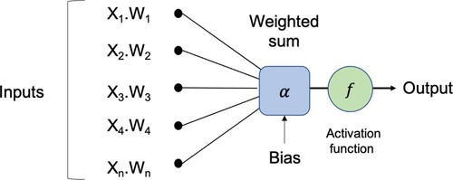
Figure 2 presents the multi-layered feed-forward neural network (MLP-NN), which consists of many layers. Layer 1 includes an input layer that matches the feature space and is followed by multiple nonlinearity layers. The final layer includes an output layer that matches the output space.

Figure 2. Multi-layer perceptron (MLP-NN) basic Architecture.

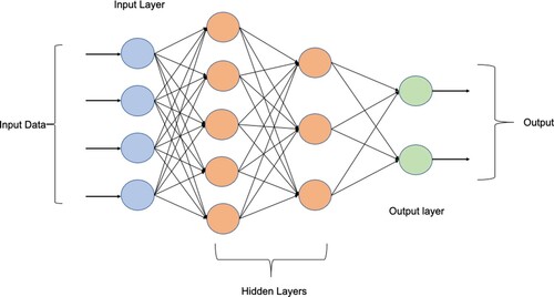
This primary architecture of the multi-layered neural networks will be used for carrying out the necessary DL tasks. The DL frameworks are regarded as models for hierarchical feature extraction, containing many nonlinearity levels. DL models have been shown to learn useful representations of raw data and perform well in dealing with complex engineering problems related to water resources management (Van et al., 2020).

4. Ensemble deep learning model

Bootstrap Aggregating (Bagging) is seen to be a Machine Learning (ML)-based meta-algorithm that could be used for improving the classification and the regression models with regards to their classification accuracy and stability (Pham et al., 2019). This model decreased the variance and prevented overfitting. Though it is generally used for decision tree models, it is compatible with several other model types. The idea of the bagging model (averaging for the regression problems having a continuous dependent variable of interest) is useful to predictive data mining. This combined the predicted classification (prediction) from various models or similar model types that are used for learning data. This model can be used for addressing the inherently unstable results noted when using complex models for a smaller data set (Dou et al., 2020). Presume that the data mining task involves building a model for predictive classification, where the dataset used for training the model (i.e. the learning data set that contains an observed classification) was small. The researcher can constantly sub-sample (using replacement) from this dataset and use a tree classifier (like CHAID) for the subsequent samples. Practically, different trees are grown for different samples, which indicates the uncertainty of the models noted in smaller datasets. One technique that is used for deriving the single prediction (for newer observations) included the use of all trees for the different samples and thereafter applying a simple voting process. Different trees predict the final classification. It should be noted that some of the weighted combinations of predictions (i.e. weighted vote or weighted average) could be derived and used. For the regression problems, the bootstrap aggregating has a similar procedure to produce a sub-set for samples based on the sampling rate and the number of iterations then all these sub-set delivered to the sub DL models to be trained individually. The final step is the aggregating by taking the mean predictions of models.

Ensemble Theory: Bagging is seen to be an ensemble technique. The Ensemble technique applies several models for acquiring a better predictive performance compared to what can be derived from the constituent models. An ensemble refers to a technique that combined several weak learners for developing a stronger learner. Evaluation of the prediction of the ensemble needs higher computation than the evaluation of one model. Hence, the ensembles are regarded as a technique that compensates for the poor learning algorithms (Yariyan et al., 2020).

Ensemble learning is a supervised learning algorithm in which multiple learning algorithms can be combined to make predictions. The trained ensemble represented one hypothesis. However, this hypothesis was not included in the hypothesis space of different models from which it was developed. Hence, ensembles display higher flexibility of functions that they represented. A few ensemble techniques (like bagging) decrease the issues related to the over-fitting of training data (Dou et al., 2020); hence, in this study, bagging techniques are developed to predict groundwater fluctuations.

5. Materials and methods

5.1. Case study

Selangor is a province that is located on the west coast of Peninsular Malaysia. It is one of Malaysia's warmest states, with high humidity and high temperature throughout the year. As the largest state economically, Selangor contains different industries that operate within. It is considered one of the country's states with multiple dry spells and faced severe water crises in the past. This study focuses on the southern part of Selangor, shown in Figure 3.

Figure 3. Map of the study area, showing the location of the observed wells.

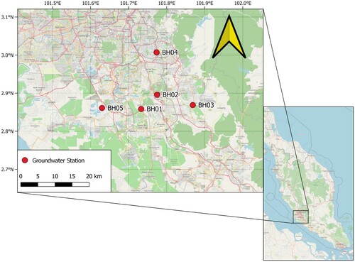
The study was conducted to predict the GWLs in five wells Jenderam Huzaifah (BH01), Bangi Lima (BH02), Beranag (BH03), Anak Yatim (BH04), and Paya Indah Wetland (BH05), which are located in different towns within Selangor (Jenderam, Bangi, Beranag, Kajang and Paya Indah Wetland) respectively. Two modeling techniques, DL and EDL, are applied to improve GWL estimation. To predict the groundwater levels, two scenarios are proposed, first scenario (S1): the 4 inputs are the GWL of the 4 wells (at the same point in time), and the output is the GWL of the remaining well (at the same point in time) and second scenario (S2): time series with lag time up to 20 days of GWL records in advance are used as inputs to predict the next day of GWL for all five wells individually. Table 1 shows summary statistics of the GWL in the wells under study which are used as an input for the models. This input data was normalized using the Z Transformation method, which is also called statistical normalization. The above normalization can subtract the average value from the data and divides it by standard deviation. The data used in this study was measured on a daily basis from 2017 until mid of 2018. the dataset will be divided into two subsets: 70% of the dataset will be used to train the proposed models, while 30% will be used to test the proposed models’ reliability. The data for all wells were taken at the same time period started at 20 October 2017–22 July 2018. The total record is 276, first 70% (194 records) taken as a training set from 20 October 2017 to 1 May 2018 and 30% (82 records) taken as testing set from 2 May 2018 to 22 July 2018.

Table 1. Descriptive statistics of the GWL in the wells under study.

Statistical parameter	BH01	BH02	BH03	BH04	BH05
Mean	17.10	15.307	16.363	13.996	16.389
Standard Error	0.027	0.018	0.008	0.014	0.0103
Median	17.065	15.23	16.35	13.92	16.34
Mode	17	15.17	16.37	13.85	16.26
Standard Deviation	0.449	0.299	0.135	0.228	0.171
Sample Variance	0.202	0.089	0.018	0.052	0.029
Kurtosis	−0.777	2.966	0.013	4.458	−0.912
Skewness	0.331	1.596	0.476	1.826	0.486
Range	1.83	1.6	0.68	1.57	0.64
Minimum	16.37	14.91	16.08	13.65	16.12
Maximum	18.2	16.51	16.76	15.22	16.76

5.2. Models development process

In this study, with regards to the development of DL models, a supervised protocol will be used for the pre-training phase in developing the DL model during the initialization step. Mean square error (MSE) will be used as a loss function to choose the best model after examining different activation functions. Lasso and ridge techniques will be used for regularization purposes to avoid the proposed model from the overfitting problem. And finally, the grid search method will be used for hyper-parameters optimization.

Regarding the development of EDL, Bagging technique is used to predict groundwater levels. Three steps will be used to develop this model. The dataset will be divided into a smaller subset, which is called the Bootstrap sample. The second step is where the bootstrap samples will be used to train the Machine Learning (ML) algorithms. The sampling rate used to be 0.1 and the number of iterations is 50 where a higher number of iterations and less sampling rate may cause more time consuming for training. Thus, 50 sub-deep learning models are created. The final step will be the aggregation, where it will be used to generate all possible outcomes and randomize the outcome. Finally, in this study Boosting Process will be introduced as a sophisticated algorithm for deriving weights for the weighted prediction.

The structure of the proposed two models can be seen in Figure 4. The first phase is to apply pre-processing; the input data will be normalized using the Z Transformation method, which is also called statistical normalization. The above normalization can subtract the average value from the data and divides it by standard deviation. Since the prediction models’ performance depends on the proper input selection and optimum values for internal parameters, selecting the best time lags is essential. Therefore, in this study, different sliding time windows are examined where the window size (time lag) ranged between 1-day and 20-day. In the second phase, the dataset will be divided into two subsets: 70% of the dataset will be used to train the proposed models, while 30% will be used to test the proposed models’ reliability. The third phase will be introduced to develop the proposed models: DL and EDL. During this phase, the hyper-parameters initialization and optimization will be examined. Table 2 shows the parameters set up for the proposed DL and the EDL models.

Figure 4. Deep learning and Ensemble Deep learning model structure-based windowing.

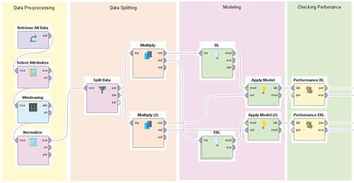
Table 2. Parameter setup for DL and EDL.

Parameter Set
Activation function	Exp Rectifier	Momentum ramp	1,000,000.0
Hidden layer sizes	50,50	Momentum stable	0.0
Reproducible_ (uses_1_thread)	false	Nesterov accelerated gradient	True
Use local random seed	false	Standardize	True
Local random seed	1992	L1	1.0E-5
epochs	100.0	L2	0.0
Compute variable importance	false	Max_w2	10.0
Train samples per iteration	−2	Loss function	Automatic
Adaptive rate	true	Distribution function	AUTO
epsilon	1.0E-8	Early stopping	False
rho	0.99	Stopping rounds	1
Learning rate	0.005	Stopping metric	AUTO
Learning rate annealing	1.0E-6	Stopping tolerance	0.001
Learning rate decay	1.0	Missing values handling	Mean Imputation
Momentum start	0.0

During the final phase, models need to be assessed for their performance to make sure they are reliable for implementation. To do so, the predicted outputs of each model are compared with the observed measurements of the groundwater levels in the wells. A total of 13 statistical indices were computed to evaluate the models as can be seen in Table 3.

Table 3. Selected performance indicators.

Equation	Performance indicator
$RMSE=\sqrt{{\displaystyle \frac{1}{n}}\sum _{i=1}^n{(y_i-\widehat{y_i})}^2}$	Root mean squared error, RMSE (Adamowski & Chan, 2011) presents the discrepancy existing between the observed and predicted values.
$AE={\displaystyle \sum _{i=1}^n|y_i-\widehat{y_i}|}$	Absolute error, AE is the measure of Absolute difference presented between the predicted and observed values.
$RE={\displaystyle \sum _{i=1}^n{\displaystyle \frac{|y_i-\widehat{y_i}|}{y_i}}}$	Relative error, RE refers to the absolute difference between the predicted and observed values divided by Observed Value.
$R{E}_L={\displaystyle \sum _{i=1}^n{\displaystyle \frac{|y_i-\widehat{y_i}|}{max(|y_i|,|\widehat{y_i}|)}}}$	Relative error lenient, REL represents the Absolute Deviation of prediction from Observed, divided by the maximal value between the Observed and Predicted values.
$R{E}_S={\displaystyle \sum _{i=1}^n{\displaystyle \frac{|y_i-\widehat{y_i}|}{min(|y_i|,|\widehat{y_i}|)}}}$	Relative error strict, RES indicates the Absolute Deviation of prediction from Observed value, divided by the minimal value between the Observed and Predicted values.
$NAE={\displaystyle \frac{AE}{{\displaystyle \frac{1}{n}}\sum _{i=1}^n|y_i|}}$	Normalized Absolut error, NAE represents the absolute difference between the observed and predicted values divided by the error noted if the average was predicted.
$RRSE=\sqrt{{\displaystyle \frac{\sum _{i=1}^n{(y_i-\widehat{y_i})}^2}{\sum _{i=1}^n{(y_i-\overline{y_i})}^2}}}$	Root relative squared error, RRSE indicates the sum of the squared error. It normalizes the squared error after dividing the total squared error for the simple predictor. After considering the square root of the RSE, the error is decreased to a similar dimension as the value that is predicted.
$SE={\displaystyle \frac{1}{n}}\sum _{i=1}^n(y_i-\widehat{y_i}{)}^2$	Squared error, SE refers to the average squared difference between the observed and predicted values.
$R={\displaystyle \frac{\sum _{i=1}^n(y_i-\overline{y_i})(\widehat{y_i}-\overline{\widehat{y_i}})}{\sqrt{\sum _{i=1}^n{(y_i-\overline{y_i})}^2}\sqrt{\sum _{i=1}^n{(\widehat{y_i}-\overline{\widehat{y_i}})}^2}}}$	Pearson correlation coefficient, R determines the strength of a linear relationship between the predicted and observed values.
$R^2=1-{\displaystyle \frac{\sum _{i=1}^N{(y_i-\widehat{y_i})}^2}{\sum _{i=1}^N{(y_i)}^2-{\displaystyle \frac{\sum _{i=1}^N{(\widehat{y_i})}^2}{N}}}}$	Coefficient of determination, R^2 is the measure of correlation existing between the observed and predicted values. It ranged between 0 and 1 (Adamowski & Chan, 2011).
$\text{Prediction average}={\displaystyle \frac{\sum _{i=1}^n(\widehat{y_i})}{n}}$	Prediction average indicates the sum of the predicted values divided by total no. of predictions.
$\text{spearman rho}=1-{\displaystyle \frac{6\times D_a^2}{A(A^2-1)}}$	Spearman rho is the non-parametric correlation measure. It can measure the linear relationship occurring between 2 variables. Da indicates the difference between the predicted and observed values.
Kendall tau	Kendall tau, represents the rank correlation occurring between the predicted and observed values. It determines the relationship strength between the predicted and observed values.

6. Results and discussion

Table 4 sum up the test results of the two deep learning methods in estimation of GWL (S1) and compare them with respect to 13 evaluation statistics. All the statistics agree that the EDL generally performs superior to the DL in the estimation of GWL of each station using data of remaining four wells except the Paya Indah Wetland in which the DL method provide better estimates compared to EDL; improvement in RMSE, NAE, RRMSE, R, Spearman rho and Kendall tau by 30.3%, 17.1%, 30.2%, 15.4%, 20.3%, and 22.5% using DL method, respectively. However, in Anak Yatim, EDL decreases RMSE from 0.169 to 0.160 by 5.3%, decreases NAE from 0.658 to 0.578 by 12.2%, decreases RRMSE from 0.649 to 0.614 by 5.4%, increases R from 0.792 to 0.811 by 2.4%, increases Spearman rho from 0.633 to 0.646 to 0.454 by 2.1, increases Kendall tau from 0.454 to 0.472 by 4%. Similarly, by applying the EDL method, in Berenang; decrement in RMSE, NAE and RRMSE are by 26.6%, 21.5% and 26.4% and increments in R, Spearman rho and Kendall tau by 10.3%, 3.2% and 5.3%; in Jenderam Huzaifah; decrement in RMSE, NAE and RRMSE are by 26.6%, 18.8% and 26.5% and increments in R, Spearman rho and Kendall tau by 14%, 7.5%, and 9.1%; in Bangi Lima; decrement in RMSE, NAE and RRMSE are by 24.9%, 17.6% and 24.8% and increments in R, Spearman rho and Kendall tau by 9.9%, 6.7%, and 11.8%, respectively.

Table 4. Deep learning and ensemble deep learning models’ performance based on the first scenario.

		Deep Learning Model					Ensemble Deep Learning Model
	Stations	Anak Yatim	Paya Indah Wetland	Beranang	Jenderam Huzaifah	Bangi Lima	Anak Yatim	Paya Indah Wetland	Beranang	Jenderam Huzaifah	Bangi Lima
	Root mean squared error (RMSE)	0.169	0.138	0.094	0.349	0.193	0.16	0.198	0.069	0.256	0.145
	Absolute error (AE)	0.120±0.118	0.117±0.073	0.072±0.060	0.265±0.228	0.130±0.143	0.105±0.120	0.141±0.138	0.057±0.040	0.215±0.139	0.107±0.098
	Relative error (RE)	0.85%±0.81%	0.71%±0.44%	0.44%±0.36%	1.56%±1.35%	0.84%±0.89%	0.74%±0.81%	0.86%±0.83%	0.35%±0.24%	1.27%±0.83%	0.69%±0.61%
	Relative error lenient (REL)	0.84%±0.80%	0.71%±0.44%	0.44%±0.36%	1.53%±1.31%	0.83%±0.88%	0.74%±0.81%	0.86%±0.83%	0.34%±0.24%	1.25%±0.81%	0.69%±0.61%
	Relative error strict (RES)	0.86%±0.83%	0.72%±0.45%	0.44%±0.37%	1.57%±1.37%	0.85%±0.92%	0.75%±0.84%	0.87%±0.86%	0.35%±0.24%	1.27%±0.84%	0.70%±0.63%
	Normalized absolute error (NAE)	0.658	0.756	0.708	0.693	0.55	0.578	0.912	0.556	0.563	0.453
	Root relative squared error (RRMSE)	0.649	0.774	0.708	0.784	0.614	0.614	1.109	0.521	0.576	0.462
	Squared error	0.028±0.071	0.019±0.020	0.009±0.018	0.122±0.181	0.037±0.090	0.025±0.078	0.039±0.066	0.005±0.006	0.066±0.079	0.021±0.046
	Correlation (R)	0.792	0.637	0.776	0.722	0.809	0.811	0.552	0.856	0.823	0.889
	Squared correlation (R2)	0.627	0.406	0.602	0.521	0.655	0.658	0.305	0.733	0.677	0.79
	Prediction average	13.989±0.260	16.390±0.178	16.374±0.132	17.069±0.445	15.320±0.314	13.989±0.260	16.390±0.178	16.374±0.132	17.069±0.445	15.320±0.314
	Spearman rho	0.633	0.539	0.779	0.724	0.827	0.646	0.448	0.804	0.778	0.882
	Kendall tau	0.454	0.386	0.602	0.547	0.638	0.472	0.315	0.634	0.597	0.713
Performance indicators

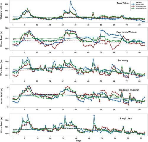
Figure 5 compares the time variation of actual and estimated GWL using DL and EDL models for the first scenario. As evident from the graphs, EDL estimates are closer to the actual data compared to the DL model.

Figure 5. Actual versus estimated water level for DL and EDL models for first scenario.

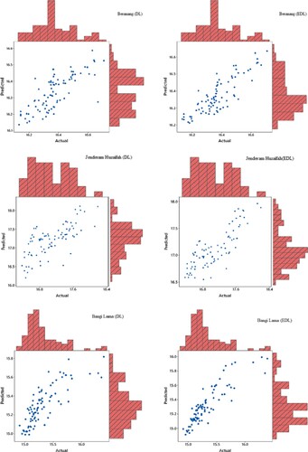
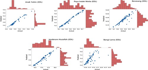
Marginal plots of the actual and estimated GWL data of each station are illustrated in Figure 6. By this plotting, distributions of the both actual and estimated values can also be observed. Marginal histograms were added to the scatter plot to visualize the distribution of the actual and predicted data. From the Figure 6, it can be said that the EDL model produced less scattered estimates and the distributions of actual and estimates by this model are more similar to each other compared to DL model.

Figure 6. Marginal plot for actual versus estimated values for the first scenario.

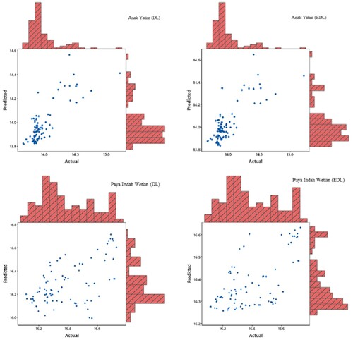
Figure 6b. Continued.

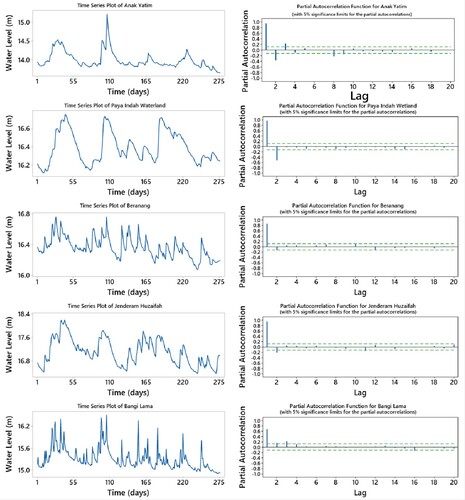
For the second scenario, partial auto-correlation functions (PCF) were analyzed to decide optimal inputs to the DL models to predict the GWL of each well. Time series plot and PCF are illustrated in Figure 7. First, the lagged inputs having significantly high correlations at the level of 5% were considered for the models, however, these inputs provided less accuracy. Then, low correlated lags were also included as inputs and obtained better accuracy. It should be noted here that eliminating some lags considering PCF is not a good idea in modeling with DL because eliminating lags may carry some important information which cannot be detected by the PCF. In addition, adding higher lagged inputs may reduce the weights DL models and provide better learning the investigated phenomenon. The PCF test has been used to illustrate the correlation of 20-day lags of GWL. A 20-day lags are used in the second scenario as inputs. The best inputs lags are selected by developing up to 200 models for both DL and EDL for each station.

Figure 7. Time series plot with partial autocorrelation for all wells.

The results of the DL models in predicting (S2) GWL of five stations are summed up in Table 5, As clearly seen from 13 statistics, the EDL had superior performance in predicting daily GWL in all five stations compared to DL model. Implementing EDL decreased the RMSE, NAE and RRMSE from 0.043, 0.249, and 0.242 to 0.038, 0.181, and 0.188 by 11.6%, 27.3% and 22.3% and increased the R, Spearman rho and Kendall tau from 0.978, 0.935, and 0.807 to 0.982, 0.945, and 0.835 by 0.4%, 1.1%, and 3.5%, respectively. Similarly, by implementing EDL, reduction in RMSE, NAE and RRMSE are by 12%, 8.3% and 13.7% and increments in R, Spearman rho and Kendall tau by 0.3%, 0.6%, and 2.5%; in Paya Indah Wetland; reduction in RMSE, NAE and RRMSE are by 21.5%, 9.9%, and 10.6% and increments in R, Spearman rho and Kendall tau by 4.9%, 3.6%, and 10.7%; in Beranang; reduction in RMSE, NAE and RRMSE are by 13.4%, 11.7%, and 16.7% and increments in R, Spearman rho and Kendall tau by 1.8%, 2.1%, and 2.4%; in Jenderam Huzaifah; reduction in RMSE, NAE and RRMSE are by 9.8%, 10.4%, and 5% and increments in R, Spearman rho and Kendall tau by 11.7%, 5.1%, and 10.3%; in Bangi Lima, respectively.

Table 5. Deep learning and ensemble deep learning models’ performance based on the second scenario.

		Deep Learning Model					Ensemble Deep Learning Model
	Stations	Anak Yatim	Paya Indah Wetland	Beranang	Jenderam Huzaifah	Bangi Lima	Anak Yatim	Paya Indah Wetland	Beranang	Jenderam Huzaifah	Bangi Lima
	Root mean squared error (RMSE)	0.043	0.025	0.065	0.127	0.205	0.038	0.022	0.051	0.11	0.185
	Absolute error (AE)	0.032±0.029	0.016±0.019	0.048±0.044	0.099±0.080	0.163±0.125	0.027±0.027	0.018±0.014	0.040±0.032	0.090±0.062	0.143±0.117
	Relative error (RE)	0.23%±0.21%	0.10%±0.11%	0.30%±0.27%	0.58%±0.46%	1.06%±0.78%	0.19%±0.19%	0.11%±0.08%	0.24%±0.20%	0.53%±0.36%	0.93%±0.73%
	Relative error lenient (REL)	0.23%±0.21%	0.10%±0.11%	0.29%±0.27%	0.58%±0.46%	1.05%±0.78%	0.19%±0.19%	0.11%±0.08%	0.24%±0.20%	0.53%±0.36%	0.92%±0.72%
	Relative error strict (RES)	0.23%±0.21%	0.10%±0.12%	0.30%±0.27%	0.58%±0.47%	1.07%±0.81%	0.19%±0.19%	0.11%±0.08%	0.24%±0.20%	0.53%±0.37%	0.94%±0.75%
	Normalized absolute error (NAE)	0.249	0.108	0.477	0.291	0.874	0.181	0.117	0.43	0.257	0.783
	Root relative squared error (RRMSE)	0.242	0.146	0.489	0.311	0.797	0.188	0.126	0.437	0.259	0.757
	Squared error	0.002±0.003	0.001±0.002	0.004±0.009	0.016±0.033	0.042±0.096	0.001±0.004	0.001±0.001	0.003±0.006	0.012±0.020	0.034±0.084
	Correlation (R)	0.978	0.99	0.876	0.953	0.648	0.982	0.993	0.919	0.97	0.724
	Squared correlation (R2)	0.956	0.981	0.768	0.909	0.42	0.965	0.987	0.844	0.941	0.525
	Prediction average	13.973±0.179	16.412±0.171	16.359±0.134	17.097±0.409	15.276±0.257	13.982±0.203	16.387±0.178	16.351±0.117	17.081±0.423	15.285±0.244
	Spearman rho	0.935	0.987	0.878	0.94	0.764	0.945	0.993	0.91	0.96	0.803
	Kendall tau	0.807	0.921	0.726	0.831	0.602	0.835	0.944	0.804	0.851	0.664
Performance indicators

Figures 8 and 9 illustrate the actual and predicted GWL by DL and EDL in the form of hydrograph. It can be apparently observed from the figures that the predictions produced by the EDL model are closer to the corresponding actual GWL data in all stations compared to DL model. Marginal plots of the implemented are compared in Figures 10 and 11. The graphs clearly show that the DL predictions are more scattered than the EDL and the similarity are higher for the EDL model. Both models gave the worst predictions for the Bangi Lima well. The reasons for this might be the lower autocorrelation and the sudden changes in the GWL as also observed from the Figure 7. As observed from Figure 7, there are sudden jumps and from low values to peaks and sudden drops from peaks to low values. This might have caused additional difficulties in learning (training) process of the DL methods.

Figure 8. Actual versus predicted water level for DL models for the second scenario.

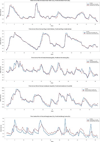
Figure 9. Actual versus predicted water level for EDL models for the second scenario.

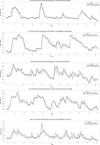
Figure 10. Marginal plot for actual versus predicted values for DL models of the second scenario.

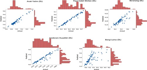
Figure 11. Marginal plot for actual versus predicted values for EDL models of the second scenario.

Finally, since the prediction models’ performance depends on the proper input selection and optimum values for internal parameters, selecting the best time lags is essential. Therefore, in this study, different sliding time windows are examined where the window size (time lag) ranged between 1-day and 20-day. Sensitivity analysis based on root mean square error (RMSE) is used to find the best time lag for each model (DL and EDL). It can be seen from Figure 12 that the EDL generally has lower RMSE than the DL in daily GWL prediction for most of the time lag selections in almost all the stations. The model exhibits a high level of precision within less time lag, ranging between 2 and 4. Table 6 shows the best time lag for each station.

Figure 12. RMSE versus window size (time lag).

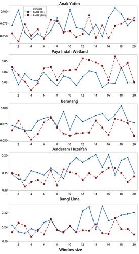
Table 6. Best time lag for each station.

	Best windowing size (No. of Lags)
Station	DL	EDL
Anak Yatim	4	2
Paya Indah Wetland	15	4
Beranang	4	4
Jenderam Huzaifah	3	3
Bangi Lima	3	4

7. Conclusion

Groundwater plays a significant role in today’s world as it counts for a large percentage of freshwater. Thus, an accurate prediction of groundwater levels has become an important aspect of industrial and urban project planning. The current study was conducted to predict the groundwater levels in 5 wells located in different towns in the state of Selangor, Malaysia, as they have faced continuous dry spells in recent years. A proposed ensemble DL model was developed, with its performance compared to a DL model's performance. The two models were developed based on two different input scenarios to predict the groundwater levels. In The first scenario, groundwater levels in one well were to be predicted using the groundwater levels in the remaining four wells, and in the second scenario, the groundwater levels in each well were to be predicted using up to 20-day time lag. Based on the results in the first scenario, the ensemble DL model outperformed the DL models in four out the five locations, however in Paya Indah Wetland well, the DL model had a better performance as it had a lower root mean squared error, lower absolute error, and lower squared error, as well as higher correlation. While in the second scenario, the ensemble model outperformed the DL model in all locations. The findings of these results indicate ensemble DL can be a reliable tool for predicting groundwater level. However, further investigations are recommended by hybridizing the EDL model to improve prediction performance such as Genetic-ensemble DL or using different meteorological and hydrological variables such as rainfall, temperature, evapotranspiration, and solar radiation inputs. Additionally, an enhancement of the results could be expected if a longer historical data were utilized in the modeling. The proposed models in this study were developed based on Malaysia's available groundwater level data. Therefore, the proposed models’ reliability could be validated in future work by using data from different regions with different climate conditions and compare it with advanced artificial intelligence models such as extreme learning machines and hybrid models.

Acknowledgements

The authors would like to thank National Hydraulic Research Institute of Malaysia (NAHRIM) for providing the data to conduct this study.

Disclosure statement

No potential conflict of interest was reported by the author(s).

References

- Adamowski, J., & Chan, H. F. (2011). A wavelet neural network conjunction model for groundwater level forecasting. Journal of Hydrology, 407(1–4), 28–40. https://doi.org/https://doi.org/10.1016/j.jhydrol.2011.06.013
- Alizamir, M., Kisi, O., Ahmed, A. N., Mert, C., Fai, C. M., Kim, S., Ahmed, A. N., Mert, C., Fai, C. M., Kim, S., Kim, N. W., & El-Shafie, A. (2020). Advanced machine learning model for better prediction accuracy of soil temperature at different depths. PLoS ONE, 15(4), e0231055. https://doi.org/https://doi.org/10.1371/journal.pone.0231055
- Baek, Y., & Kim, H. Y. (2018). Modaugnet: A new forecasting framework for stock market index value with an overfitting prevention LSTM module and a prediction LSTM module. Expert Systems with Applications, 113, 457–480. https://doi.org/https://doi.org/10.1016/j.eswa.2018.07.019
- Banadkooki, F. B., Ehteram, M., Ahmed, A. N., Teo, F. Y., Fai, C. M., Afan, H. A., Sapitang, M., & El-Shafie, A. (2020). Enhancement of groundwater-level prediction using an integrated machine learning model optimized by whale algorithm. Natural Resources Research, 29(5), 3233–3252. https://doi.org/https://doi.org/10.1007/s11053-020-09634-2
- Barzegar, R., Fijani, E., Asghari Moghaddam, A., & Tziritis, E. (2017). Forecasting of groundwater level fluctuations using ensemble hybrid multi-wavelet neural network-based models. Science of The Total Environment, 599–600, 20–31. https://doi.org/https://doi.org/10.1016/j.scitotenv.2017.04.189
- Bryngelson, S. H., Charalampopoulos, A., Sapsis, T. P., & Colonius, T. (2020). A Gaussian moment method and its augmentation via LSTM recurrent neural networks for the statistics of cavitating bubble populations. International Journal of Multiphase Flow, 127, 103262. https://doi.org/https://doi.org/10.1016/j.ijmultiphaseflow.2020.103262
- Candel, A., Ledell, E., & Bartz, A. (n.d.). Deep learning with H2O. http://h2o.ai/resources/
- Chang, F. J., Chang, L. C., Huang, C. W., & Kao, I. F. (2016). Prediction of monthly regional groundwater levels through hybrid soft-computing techniques. Journal of Hydrology, 541, 965–976. https://doi.org/https://doi.org/10.1016/j.jhydrol.2016.08.006
- Chitsazan, M., Rahmani, G., & Neyamadpour, A. (2015). Forecasting groundwater level by artificial neural networks as an alternative approach to groundwater modeling. Journal of the Geological Society of India, 85(1), 98–106. https://doi.org/https://doi.org/10.1007/s12594-015-0197-4
- Choubin, B., Hosseini, F. S., Fried, Z., & Mosavi, A. (2020). Application of Bayesian regularized neural networks for groundwater level modeling. CANDO-EPE 2020 - Proceedings, IEEE 3rd International Conference and Workshop in Obuda on Electrical and Power Engineering (pp. 209–212). https://doi.org/https://doi.org/10.1109/CANDO-EPE51100.2020.9337753
- Choubin, B., & Malekian, A. (2017). Combined gamma and M-test-based ANN and ARIMA models for groundwater fluctuation forecasting in semiarid regions. Environmental Earth Sciences, 76(15), 1–10. https://doi.org/https://doi.org/10.1007/s12665-017-6870-8
- Choubin, B., & Rahmati, O. (2021). Groundwater potential mapping using hybridization of simulated annealing and random forest. In P. Samui, H. Bonakdari, & R. Deo (Eds.), Water engineering modeling and mathematic tools (pp. 391–403). Elsevier. https://doi.org/https://doi.org/10.1016/b978-0-12-820644-7.00008-6
- Demirci, M., Üneş, F., & Körlü, S. (2019). Modeling of groundwater level using artificial intelligence techniques: A case study of Reyhanli region in Turkey. Applied Ecology and Environmental Research, 17(2), 2651–2663. https://doi.org/https://doi.org/10.15666/aeer/1702_26512663
- Dou, J., Yunus, A. P., Bui, D. T., Merghadi, A., Sahana, M., Zhu, Z., Chen, C-W., Han, Z., & Pham, B. T. (2020). Improved landslide assessment using support vector machine with bagging, boosting, and stacking ensemble machine learning framework in a mountainous watershed. Japan. Landslides, 17(3), 641–658. https://doi.org/https://doi.org/10.1007/s10346-019-01286-5
- Hoque, M. A., & Adhikary, S. K. (2020, February). Prediction of groundwater level using artificial neural network and multivariate timeseries models. Proceedings of the 5th International Conference on Civil Engineering for Sustainable Development (ICCESD 2020), Bangladesh. http://www.iccesd.com/
- Huang, F., Huang, J., Jiang, S. H., & Zhou, C. (2017). Prediction of groundwater levels using evidence of chaos and support vector machine. Journal of Hydroinformatics, 19(4), 586–606. https://doi.org/https://doi.org/10.2166/hydro.2017.102
- Huang, M., & Tian, Y. (2015). Prediction of groundwater level for sustainable water management in an arid basin using data-driven models. (Seee), 134–137. https://doi.org/https://doi.org/10.2991/seee-15.2015.33
- Kenda, K., Čerin, M., Bogataj, M., Senožetnik, M., Klemen, K., Pergar, P., Laspidou, C., & Mladenić, D. (2018). Groundwater modeling with Machine Learning techniques: Ljubljana polje aquifer. Proceedings, 2(11), 697. https://doi.org/https://doi.org/10.3390/proceedings2110697
- Kenda, K., Peternelj, J., Mellios, N., Kofinas, D., Čerin, M., & Rožanec, J. (2020). Usage of statistical modeling techniques in surface and groundwater level prediction. Journal of Water Supply: Research and Technology-Aqua, 69(3), 248–265. https://doi.org/https://doi.org/10.2166/aqua.2020.143
- Khaki, M., Yusoff, I., Islami, N., & Hussin, N. H. (2016). Artificial neural network technique for modeling of groundwater level in Langat basin, Malaysia. Sains Malaysiana, 45(1), 19–28.
- Kouziokas, G. N., Chatzigeorgiou, A., & Perakis, K. (2018). Multilayer feed forward models in groundwater level forecasting using meteorological data in public management. Water Resources Management, 32(15), 5041–5052. https://doi.org/https://doi.org/10.1007/s11269-018-2126-y
- Lai, V., Ahmed, A. N., Malek, M. A., Abdulmohsin Afan, H., Ibrahim, R. K., El-Shafie, A., & El-Shafie, A. (2019). Modeling the nonlinearity of sea level oscillations in the Malaysian coastal areas using machine learning algorithms. Sustainability, 11(17), 4643. https://doi.org/https://doi.org/10.3390/su11174643
- Li, H., Lu, Y., Zheng, C., Yang, M., & Li, S. (2019). Ground water level prediction for the arid oasis of Northwest China based on the artificial bee colony algorithm and a back-propagation neural network with double hidden layers. Water, 11(4), 860–820. https://doi.org/https://doi.org/10.3390/w11040860
- Li, Z., Yang, Q., Wang, L., & Martín, J. D. (2017). Application of RBFN network and GM (1, 1) for groundwater level simulation. Applied Water Science, 7(6), 3345–3353. https://doi.org/https://doi.org/10.1007/s13201-016-0481-5
- Lohani, A., & Krishan, G. (2015). Groundwater level simulation using artificial neural network in southeast, punjab, India. Journal of Geology & Geophysics, 4, 3. https://doi.org/https://doi.org/10.4172/2381-8719.1000206
- Massaoudi, M., Chihi, I., Sidhom, L., Trabelsi, M., Refaat, S. S., Abu-Rub, H., & Oueslati, F. S. (2021). An effective hybrid NARX-LSTM model for point and interval PV power forecasting. IEEE Access, 9, 36571–36588. https://doi.org/https://doi.org/10.1109/ACCESS.2021.3062776
- Mosavi, A., Hosseini, F. S., Choubin, B., Abdolshahnejad, M., Gharechaee, H., Lahijanzadeh, A., & Dineva, A. A. (2020). Susceptibility prediction of groundwater hardness using ensemble machine learning models. Water, 12(10), 2770. https://doi.org/https://doi.org/10.3390/w12102770
- Mosavi, A., Sajedi Hosseini, F., Choubin, B., Goodarzi, M., Dineva, A. A., & Rafiei Sardooi, E. (2021a). Ensemble boosting and Bagging based machine learning models for groundwater potential prediction. Water Resources Management, 35(1), 23–37. https://doi.org/https://doi.org/10.1007/s11269-020-02704-3
- Mosavi, A., Sajedi Hosseini, F., Choubin, B., Taromideh, F., Ghodsi, M., Nazari, B., & Dineva, A. A. (2021b). Susceptibility mapping of groundwater salinity using machine learning models. Environmental Science and Pollution Research, 28(9), 10804–10817. https://doi.org/https://doi.org/10.1007/s11356-020-11319-5
- Najah, A., El-Shafie, A., Karim, O. A., Jaafar, O., & El-Shafie, A. H. (2011). An application of different artificial intelligences techniques for water quality prediction. International Journal of Physical Sciences, 6(22), 5298–5308. https://doi.org/https://doi.org/10.5897/IJPS11.1180
- Natarajan, N., & Sudheer, C. (2020). Groundwater level forecasting using soft computing techniques. Neural Computing and Applications, 32(12), 7691–7708. https://doi.org/https://doi.org/10.1007/s00521-019-04234-5
- Osman, A. I. A., Ahmed, A. N., Chow, M. F., Huang, Y. F., & El-Shafie, A. (2021). Extreme gradient boosting (xgboost) model to predict the groundwater levels in Selangor Malaysia. Ain Shams Engineering Journal, 12(2), 1545–1556. https://doi.org/https://doi.org/10.1016/j.asej.2020.11.011
- Pham, B. T., Jaafari, A., Prakash, I., Singh, S. K., Quoc, N. K., & Bui, D. T. (2019). Hybrid computational intelligence models for groundwater potential mapping. Catena, 182, 104101. https://doi.org/https://doi.org/10.1016/j.catena.2019.104101
- Pourghasemi, H. R., Sadhasivam, N., Yousefi, S., Tavangar, S., Ghaffari Nazarlou, H., & Santosh, M. (2020). Using machine learning algorithms to map the groundwater recharge potential zones. Journal of Environmental Management, 265, 110525. https://doi.org/https://doi.org/10.1016/j.jenvman.2020.110525
- Sahoo, S., & Jha, M. K. (2015). On the statistical forecasting of groundwater levels in unconfined aquifer systems. Environmental Earth Sciences, 73(7), 3119–3136. https://doi.org/https://doi.org/10.1007/s12665-014-3608-8
- Sattari, M. T., Mirabbasi, R., Sushab, R. S., & Abraham, J. (2018). Prediction of groundwater level in Ardebil plain using support vector regression and M5 tree model. Groundwater, 56(4), 636–646. https://doi.org/https://doi.org/10.1111/gwat.12620
- Shamsuddin, M. K. N., Kusin, F. M., Sulaiman, W. N. A., Ramli, M. F., Baharuddin, M. F. T., & Adnan, M. S. (2017). Forecasting of groundwater level using artificial neural network by incorporating river recharge and river bank infiltration. MATEC Web of Conferences, 103, 04007. https://doi.org/https://doi.org/10.1051/matecconf/201710304007
- Takafuji, E. H. d. M., Rocha, M. M. d., & Manzione, R. L. (2019). Groundwater level prediction/forecasting and assessment of uncertainty using SGS and ARIMA models: A Case Study in the Bauru aquifer system (Brazil). Natural Resources Research, 28(2), 487–503. https://doi.org/https://doi.org/10.1007/s11053-018-9403-6
- Takeuchi, D., Yatabe, K., Koizumi, Y., Oikawa, Y., & Harada, N. (2020, May). Real-time speech enhancement using equilibrated RNN. ICASSP, IEEE International Conference on Acoustics, Speech and Signal Processing – Proceedings (pp. 851–855). https://doi.org/https://doi.org/10.1109/ICASSP40776.2020.9054597
- Van, S. P., Le, H. M., Thanh, D. V., Dang, T. D., Loc, H. H., & Anh, D. T. (2020). Deep learning convolutional neural network in rainfall-runoff modelling. Journal of Hydroinformatics, 22(3), 541–561. https://doi.org/https://doi.org/10.2166/hydro.2020.095
- Yadav, B., Ch, S., Mathur, S., & Adamowski, J. (2017). Assessing the suitability of extreme learning machines (ELM) for groundwater level prediction. Journal of Water and Land Development, 32(1), 103–112. https://doi.org/https://doi.org/10.1515/jwld-2017-0012
- Yadav, B., Gupta, P. K., Patidar, N., & Himanshu, S. K. (2020). Ensemble modelling framework for groundwater level prediction in urban areas of India. Science of the Total Environment, 712, 135539. https://doi.org/https://doi.org/10.1016/j.scitotenv.2019.135539
- Yang, S., & Tsai, F. T. C. (2020). Understanding impacts of groundwater dynamics on flooding and levees in Greater New Orleans. Journal of Hydrology: Regional Studies, 32, 100740. https://doi.org/https://doi.org/10.1016/j.ejrh.2020.100740
- Yariyan, P., Janizadeh, S., Van Phong, T., Nguyen, H. D., Costache, R., Van Le, H., & Tiefenbacher, J. P. (2020). Improvement of best first decision trees using Bagging and dagging ensembles for flood probability mapping. Water Resources Management, 34(9), 3037–3053. https://doi.org/https://doi.org/10.1007/s11269-020-02603-7
- Yousefi, H., Zahedi, S., Niksokhan, M. H., & Momeni, M. (2019). Ten-year prediction of groundwater level in Karaj plain (Iran) using MODFLOW2005-NWT in MATLAB. Environmental Earth Sciences, 78(12), 343. https://doi.org/https://doi.org/10.1007/s12665-019-8340-y