Flow analysis and optimization of a vertical axis wind turbine blade with a dimple

Abstract

In this study, the influences of the geometric characteristics of a dimple on the aerodynamic properties of a vertical axis wind turbine are investigated, and its configuration optimization that maximizes the wind turbine's performance is carried out. Three parameters that control the position, size and depth of the dimple are used to parameterize the dimple's configuration and to conduct optimization. With these parameters, when the flows around the wind turbines with various dimples are compared, several meaningful physical phenomena are found. First, a strong association between the position of a dimple and the power coefficient is found where the power coefficient increases as the position of the dimple approaches the trailing edge of the wind turbine blade. Second, high-performance enhancement tends to be achieved when a dimple is small, but this attribution becomes weaker as the dimple moves toward the trailing edge. Furthermore, when the flow of the optimal wind turbine is compared with the one without a dimple, a reduction of the blade wake and delay of the flow separation can be identified. Finally, the shed vortices from the optimal wind turbine blade are weaker and decay faster than the ones shed from the wind turbine without a dimple.

Keywords:

• Vertical-axis wind turbine
• dimple
• CFD simulation
• optimization
• performance improvement

1. Introduction

Generating renewable energy in urban areas has a great advantage because it makes on-site energy generation possible, hence not requiring massive energy transmission systems to transport the produced energy to the energy consumption site. Furthermore, in urban areas, plenty of wind can be generated at particular locations such as close to freeways and around tall buildings. Recycling these wasted energy sources in urban areas and producing renewable energy is highly promising from a sustainability aspect. Indeed, several researchers including Balduzzi et al. (2012), Tian et al. (2017), and Bani-Hani et al. (2018) have confirmed its feasibility.

A suitable type of wind turbine for urban area usage is a vertical axis wind turbine (VAWT). In the VAWT setup, it is possible to generate a constant power output regardless of the direction of the wind because its blades are installed perpendicular to the ground (Eriksson et al., 2008). In addition, a VAWT generates less noise (Riegler, 2003), has low construction and maintenance costs (Tjiu et al., 2015), and can generate energy at lower wind speeds than a horizontal axis wind turbine (HAWT) (Chong et al., 2013). Despite VAWT's beneficial characteristics, one obstacle hindering VAWT installation is its low efficiency in generating energy.

One factor that needs to be considered in increasing the VAWT's efficiency is how to efficiently convert from wind kinetic energy to the mechanical energy of the wind turbine, which is significantly related to the configuration of a wind turbine blade, as shown in Kang et al. (2014, december). This is because the configuration of the blade affects the essential aerodynamic features of the flow around the blade such as dynamic stall (Ferreira et al., 2009; Ma et al., 2019; McCroskey, 1981), intensity and decay rate of the shed vortex from the blade (Zhao et al., 2019), intensity of blade wakes (Brownlee, 1988; Simão Ferreira, 2009), and blade-wake interactions (Qamar & Janajreh, 2017; Scheurich et al., 2011). All of these aerodynamic features are significantly related to the wind turbine's performance, but the influences of the wind turbine's configuration on the performance and aerodynamic characteristics have been less well-studied compared with the ones for the HAWT due to the VAWT only recently being studied more.

In the present study, various configurations of VAWT blades are explored and their own performances are evaluated. Here, modification of the blade configuration is not implemented by changing the overall geometry of it but instead by mounting a dimple on the surface of the blade to make use of its effectiveness in improving the wind turbine's efficiency. Several researchers have attempted to carry out experiments and simulations in this aspect. For example, Olsman and Colonius (2011) installed a dimple on the upper side of the turbine blade airfoil and showed that the lift-to-drag ratio of the airfoil with the dimple is higher than that of the regular one. Ismail and Vijayaraghavan (2015) modified the NACA0015 wind turbine blade by mounting a dimple and vertical flap (known as a Gurney flap) and found that the modified wind turbine generates a higher lift coefficient and tangential force than the regular wind turbine. They also found that the high tangential force and low drag force are applied on the modified wind turbine due to the reduction of wake separated from the turbine. Zhu et al. (2019) simulated three modified wind turbines where two of them have a dimple-flap-combined device on the upper and lower surfaces, respectively, while the other one has the device on both sides of the surface and observed that all of these three turbines show higher power coefficients than the regular wind turbine. Sobhani et al. (2017) investigated the effects of dimples on wind turbines' aerodynamic properties by considering circular, square and triangular dimples mounted at several different locations and concluded that the performance of the wind turbine with the circular dimple located near the leading edge is the best. However, the configurations of the dimples dealt with in their study are limited and clear physical descriptions about the results are not provided.

Although these previous studies successfully showed the effectiveness of creating a dimple (or with a Gurney flap) on the wind turbine blade for performance enhancement, none of these studies investigated the influence of the dimple's parameters on the wind turbine's performance systematically. Moreover, the previous studies did not optimize the dimple's configuration for performance improvement and did not provide detailed flow comparison with corresponding physical interpretations between the wind turbines with and without the (optimal) dimple. In the current paper, CFD simulations of VAWTs with various dimples are carried out to figure out the influences of the dimple's geometric characteristics on their aerodynamic properties and optimization of the dimple's configuration is performed to maximize the turbine's performance. The type of wind turbine handled in the present study is a straight-bladed H-Darrieus wind turbine. The flow is simulated in 2D based on the fact that the longitudinal effects of the wind turbine are trivial if the blades are sufficiently long (Sobhani et al., 2017). The three-bladed NACA0021 wind turbine is chosen as the reference wind turbine because of its wide utilization in industry (Akansu et al., 2017; Tirkey et al., 2014), and a dimple is mounted on the lower surface of each of its blades. The performance of the wind turbine is evaluated with respect to the power coefficient. Three parameters that control the dimple's position, size and depth are used to vary the configuration of a dimple. The effects of these parameters are investigated at the condition where the maximum torque coefficient is measured (at the tip speed ratio $\lambda =2.5$). For optimization, a surrogate model is constructed using an artificial neural network (ANN), and a genetic algorithm is used as a searching method. As a result of optimization, the optimal wind turbine whose power coefficient is approximately $6.46\mathrm{\%}$ higher than the reference turbine is found.

The main contributions of the current study are as follows: First, the aerodynamic advantages of mounting the dimple on the surface of the wind turbine are verified, and the optimal wind turbine (the wind turbine with the optimal dimple) whose performance is enhanced at a wide range of the tip speed ratio is found. In addition, clear associations between the dimple parameters such as the dimple's position and size on the wind turbine's performance are discovered. Finally, profound physical interpretations explaining the reasons for performance enhancement in the optimal wind turbine are presented by comparing the flows between the reference and optimal wind turbines. Further descriptions regarding the present study's findings are provided in the rest of the paper.

2. Aerodynamics properties

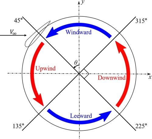
As shown in Figure 1, the path of a wind turbine's revolution can be divided into windward, upwind, leeward and downwind paths with respect to the azimuthal angle θ. The wind turbine blade shows its own aerodynamic characteristics at each of these paths. For example, as the angle of attack increases in the upwind path, the dynamic stall progresses and flow separation occurs. In the leedward, downward and windward paths, blade-wake interaction takes place as the blade passes across the wake produced by the other blades. All of these aerodynamic characteristics of the blade are complicated but important physical phenomena that should be investigated in detail.

Figure 1. Segmentation of the wind turbine path: windward, upwind, leeward and downwind regions.

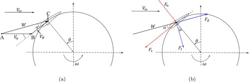
The axial flow velocity $V_a$ through the blade is the velocity component induced by the freestream velocity $V_{\mathrm{\infty }}$ (Mohammed et al., 2019). With an axial induction factor a (Beri & Yao, 2011), the axial flow velocity can be written in terms of $V_{\mathrm{\infty }}$ as (1) $V_a=V_{\mathrm{\infty }}(1-a).$(1) The axial flow velocity $V_a$ and the tangential velocity $V_{\theta }$ due to the rotation of the blade are two velocity components passing through the blade. If the relative velocity of the blade is defined as W, it can be computed by adding the velocity vectors of $V_a$ and $V_{\theta }$. This relation allows us to create the velocity triangle ABC shown in Figure 2(a), where α indicates the angle of attack of the airfoil. Applying the sine rule to the triangle gives (2) $\frac{V_a}{\sin \alpha }=\frac{V_{\theta }}{\sin (\theta -\alpha )}.$(2) With the relation of $\sin (\theta -\alpha )=\sin \theta \cos \alpha -\cos \theta \sin \alpha$, substituting it into Equation (2(2) $\frac{V_a}{\sin \alpha }=\frac{V_{\theta }}{\sin (\theta -\alpha )}.$(2) ) and multiplying $\sin \alpha$ to the equation gives (3) $V_a=\frac{V_{\theta }}{\sin \theta \cot \alpha -\cos \theta }.$(3) By rearranging Equation (3(3) $V_a=\frac{V_{\theta }}{\sin \theta \cot \alpha -\cos \theta }.$(3) ), it can be written as (4) $\tan \alpha =\frac{V_a\sin \theta }{V_{\theta }+V_a\cos \theta }.$(4) If the radius and angular velocity of the wind turbine are given as R and ω, respectively, the velocity $V_{\theta }$ can be written as $V_{\theta }=R\omega$. Then, from Equation (4(4) $\tan \alpha =\frac{V_a\sin \theta }{V_{\theta }+V_a\cos \theta }.$(4) ), the angle of attack α is derived as (5) $\alpha ={\tan }^{-1}(\frac{\sin \theta }{\frac{\lambda }{1-a}+\cos \theta }),$(5) where λ is a tip speed ratio, which is defined as (6) $\lambda =\frac{R\omega }{V_{\mathrm{\infty }}}.$(6) The resultant force applied to the blade (produced by the lift and drag of the blade) can be decomposed into the tangential and normal force components. If $C_l$ and $C_d$ denote the lift and drag coefficients of the blade, respectively, the tangential force coefficient $C_t$ and normal force coefficient $C_n$ of the blade can be derived as follows (see Figure 2(b)): (7) $\begin{array}{rl}{C}_t& =C_l\sin \alpha -C_d\cos \alpha \end{array}$(7) (8) $\begin{array}{rl}{C}_n& =C_l\cos \alpha +C_d\sin \alpha \end{array}$(8) From Equation (7(7) $\begin{array}{rl}{C}_t& =C_l\sin \alpha -C_d\cos \alpha \end{array}$(7) ), the tangential force $F_t$ generating the torque about the wind turbine's center is computed from (9) $F_t=\frac{1}{2}{C}_t\rho cH{W}^2,$(9) where ρ is air density, c is the blade chord length and H is the turbine height. Then, the torque M received by the blade can be calculated as (10) $M=F_{t}R,$(10) and the moment coefficient $C_m$ is calculated by (11) $C_m=\frac{M}{\frac{1}{2}\rho RA{V}_{\mathrm{\infty }}^2},$(11) where A is the turbine swept area. Because $C_t$ changes with respect to θ, it means the value of $F_t$ varies along the blade path. The average tangential force ${\overline{F}}_t$ on the blade for one revolution can be calculated by integrating Equation (9(9) $F_t=\frac{1}{2}{C}_t\rho cH{W}^2,$(9) ) over θ from [0, 2π]: (12) ${\overline{F}}_t=\frac{1}{2\pi }{\int }_0^{2\pi }{F}_t(\theta )\mathrm{d}\theta .$(12) With this average tangential force, the total torque Q can be calculated as (13) $Q=N\overline{F_t}R,$(13) where N is the number of blades, which is three in the present study. If A is defined as the turbine swept area, the power coefficient of the wind turbine $C_p$ is (14) $C_p=\frac{Q\omega }{\frac{1}{2}\rho A{V}_{\mathrm{\infty }}^3}.$(14)

Figure 2. Analysis of (a) velocity and (b) force on the VAWT blade.

3. Numerical approach

3.1. CFD simulation

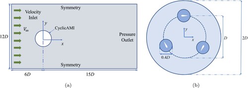
Figure 3 shows the computational domain for the wind turbine computational fluid dynamic (CFD) simulation. The total size of the computational domain is $21D$ and $12D$ in the streamwise direction (x direction) and longitudinal direction (y direction), respectively, where D is the turbine diameter. The distance from the inlet to the center of the wind turbine is $6D$, leaving a distance of $15D$ between the center of the wind turbine and the outlet of the computational domain. In the simulation, the boundaries of the computational domain should be fixed, but the wind turbine needs to rotate. To implement these simulation conditions, the mesh is decomposed into two regions. One is a stationary region that is fixed over the entire simulation and the other is a rotating region that rotates with the wind turbine. In the current paper, a circular rotating region is dealt with in which the diameter is $2D$, while the region that does not belong to the rotating region is defined as the stationary region. Around each wind turbine blade, a circular refinement region whose diameter is 0.4D is set to refine the mesh to resolve the flow properly near the blade. The velocity inlet and pressure outlet boundary conditions are used at the inlet and outlet of the computational domain, respectively. At the top and bottom surfaces, the symmetry boundary condition is applied. The no-slip condition is applied on each surface of the wind turbine blade. At the interface between the stationary and rotating regions, the cyclic arbitrary mesh interface boundary condition, which matches the physical properties across the interface, is utilized. The dynamic mesh approach is applied to make the rotating region revolve while the stationary mesh is fixed. The rotating mesh is created by using the meshing algorithm SALOME, while the stationary mesh is created by blockMesh. A structured grid with 15 layers is generated on the blade surface to capture the viscous effect of the flow near the blade's surface. The average and maximum y${}^{+}$ values of the structured grid are set to 1.04 and 3.92, respectively, which are the values that allow for capturing the effect of the wall properly. Unsteady two-dimensional Reynolds-averaged Navier-Stokes (RANS) equations are solved to simulate the flow using the open-source CFD code OpenFOAM. For turbulence modeling, the Spalart-Allmaras turbulence model is used with the kqRWallFunction and nutUSpaldingWallFunction for near-wall treatment. The PIMPLE algorithm is used with the second-order spatial discretization schemes for pressure and momentum and the first-order Gauss upwind scheme for turbulence. When the PIMPLE algorithm is used, the pressure equation is solved twice in each step for better convergence. The geometric agglomerated algebraic multi-grid solver is applied to solve algebraic equations for the pressure and the Gauss-Seidel method is used to solve for the velocity and turbulence quantities. As a time-stepping method, the Crank−Nicolson method with an off-centering coefficient of 0.9 is applied, as suggested in Greenshields (2015), to obtain better numerical stability than the pure Crank-Nicolson method (Seng et al., 2017).

Figure 3. A computational domain for the wind turbine CFD simulation. The size and boundary conditions of the stationary and rotating regions are presented in (a) and (b), respectively.

Castelli et al. (2011) carried out wind tunnel tests for the three-bladed NACA0021 wind turbine at several tip speed ratios and provided their experiment results with respect to the power coefficient. They also provided specifications of the tested wind turbine with the experimental conditions, allowing other researchers to use their experiment data for validation. With this experimental data, to verify the CFD simulations implemented in the current paper, the wind turbine that is geometrically identical to the one tested in Castelli et al. (2011) is chosen for the simulation. This three-bladed NACA0021 wind turbine will be referred to as the reference wind turbine in the rest of the current paper.

To compare the present study's simulation results with the experimental data, a grid sensitivity test was carried out in advance to find the proper mesh that would allow us to obtain reliable simulation results. For this purpose, the flow around the wind turbine with the 0.04c diameter semicircular dimple at $x_d=0.5c$ has been simulated with the four meshes created by changing the number of mesh points on the wind turbine airfoil. Table 1 shows the values of the power coefficients for these four meshes at $\lambda =2.5$. The variation of $C_p$ in the last row shows the difference of $C_p$ at the corresponding mesh with respect to the Mesh 4. As presented in the table, the variations of $C_p$ are significantly reduced from the Mesh 2. Among these four meshes, the intermediate one (Mesh 2) whose variation of $C_p$ is 0.97$\mathrm{\%}$ is used for further CFD simulations, which provides a good compromise between the simulation accuracy and computational cost efficiency.

Table 1. Change of $C_p$ at four independent meshes.

Types of mesh	Mesh 1	Mesh 2	Mesh 3	Mesh 4
Number of points on the airfoil	206	414	594	786
Number of cells	196,843	228,053	258,055	284,189
$C_p$	0.3777	0.3528	0.3485	0.3494
Variation of $C_p$ (%)	8.07	0.97	0.26	–

Note: The simulations are performed at $\lambda =2.5$ with the wind turbine having a NACA0021 airfoil profile.

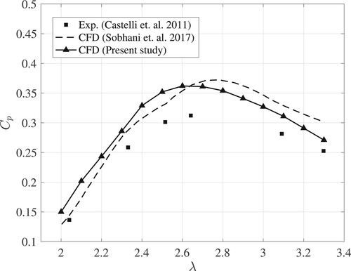
In Figure 4, the power coefficients obtained from the present study are compared with the experiment data (Castelli et al., 2011) and the CFD simulation results in Sobhani et al. (2017). The change in the power coefficients of the present study with respect to the tip speed ratio matches well with the experimental data, but the values of the current study's power coefficients are slightly higher than the ones measured from the experiment for all tip speed ratios. There are two primary reasons for this discrepancy. The first reason is because the CFD simulations conducted in the current paper are performed only with three wind turbine blades without the presence of the wind turbine's shaft. In this simulation circumstance, the kinetic energy of the wind cannot be dissipated around the shaft as it was in the experiment; therefore, the overestimated power coefficients of the present study's CFD simulations are inevitable. Despite this defect, ignoring the existence of the shaft is used for the wind turbine simulation not only in the current study, but also many other previous studies such as Castelli et al. (2011), Ma et al. (2019), Giorgetti et al. (2015) and Sobhani et al. (2017) because it allows more efficient CFD simulations with a reasonable accuracy. When the power coefficients of the present study are compared with the ones implemented by Sobhani et al. (2017) (one of the previous studies that simulated the reference wind turbine without the shaft), the two CFD simulation results show a similar order of accuracy, as shown in Figure 4. The other primary reason is the absence of tip vortices that are ignored by using 2D CFD simulations. In reality, tip vortices are generated around each end of the three wind turbine blades because of the instability of the flow at the tips. This flow instability reduces the torque produced by the wind turbine, especially around the ends of the blades, thereby reducing the overall performance of the wind turbine. However, in the present study, since 2D CFD simulations are carried out, the flow characteristics caused by the effect of the blade length cannot be sufficiently reflected in the simulations. Therefore, the flow instability existing around the ends of the blades is also ignored, which eventually leads to obtaining overestimated $C_p$ compared with the experiment data.

Figure 4. The power coefficients computed from the present study's CFD simulations are compared with the experimental data in Castelli et al. (2011) and the CFD simulation data in Sobhani et al. (2017) as a function of the tip speed ratio.

4. Optimization

To investigate influences of the configuration of a dimple on the blade's aerodynamic properties, the reference wind turbine (three-bladed NACA0021 wind turbine) is modified by mounting a dimple on the lower surface, which here refers to the suction side of the blade in the upstream region. The three parameters that control the configuration of a dimple with respect to the blade location, size and depth are introduced in the present study. With the parameters, the dimple is optimized to maximize the wind turbine's performance by dealing with the three dimple's parameters as design parameters for the optimization. The optimization is implemented under the simulation condition using the freestream velocity $V_{\mathrm{\infty }}=9$ m/s and $\lambda =2.5$. With these simulation conditions, the blade chord-based Reynolds number of the flow is $R{e}_c=1.37\times {10}^5$. The knowledge needed to understand the optimization process performed in the current paper is described in this section.

4.1. Dimple parameters

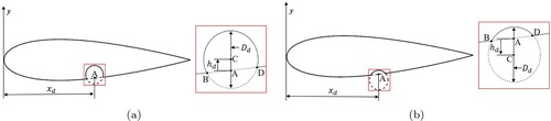
Figure 5 illustrates the three dimple's parameters ($x_d$, $D_d$ and $h_d$) considered in the current paper. The dimple location parameter $x_d$ defines the horizontal distance between the leading edge of the wind turbine airfoil and the center of the dimple, hence determining the location of the dimple on the airfoil. The diameter of the dimple's circle (the circle presented in the red box in the figure), which controls the size of the dimple, is defined as $D_d$. If point A in the figure denotes the place on the lower surface of the airfoil at $x=x_d$, the dimple's depth parameter $h_d$, which affects the aspect ratio of the dimple, is the signed distance from point A to the center of the dimple (presented as point C). Here, the value of the signed distance is positive if the center of the dimple (point C) is located above point A, leading to the generation of a thicker dimple than the one when the value is negative. Note that the dimple (arc BD plotted in solid line) is the segmentation of the dimple's circle, and the portion of the dimple in the circle is determined by the parameter $h_d$.

Figure 5. The three parameters determining the configuration of a dimple. The parameters $x_d$, $D_d$ and $h_d$ define the positions of the dimple, dimple circle's diameter and depth of the dimple, respectively. The dimples presented in (a) and (b) show the cases when the parameter $h_d$ is possitive and negative, respectively.

With these three parameters, the procedure to create a dimple on the wind turbine as follows: Based on the value of $x_d$, the location of point A is calculated by using the equation defining the NACA 0021 reference airfoil's lower surface (Moran, 2003). Then, the center of the dimple (point C) is defined by vertically moving point A by $h_d$, where the positive value of $h_d$ indicates moving the point A upward, while the negative value of $h_d$ indicates moving the point downward. Finally, computing the positions of the two contact points B and D (between the dimple's circle and the lower surface of the reference NACA0021 airfoil) enables us to define the arc BD, which is the configuration of the dimple. The effects of the parameters $x_d$, $D_d$ and $h_d$ are studied in Section 5.

4.2. Design of experiment

Understanding effects of design parameters on the engineering object's performance is crucial in the optimization process (Ez Abadi et al., 2020). Especially, the design of experiment, which generates a set of design points in the design space to test the response of the outputs as a function of the design parameters, is one of the most significant steps in the optimization. Numerous studies have investigated the methods that can represent a continuous design space with a finite number of design points (Durakovic, 2017; Kuram et al., 2013; Vicente et al., 1998). Because of the capability to efficiently represent the designated design space with a small number of design points, the D-optimal method (DuMouchel & Jones, 1994) and optimal Latin hypercube design method (Viana et al., 2010) are prominently used for the design of experiment. However, the method used in the current paper is the discrete level-based method (Oh, 2020), which distributes equally spaced design points in the design space because it has an advantage in investigating the behavior of the outputs with respect to the design parameters. Although the required number of design points in the discrete level-based method exponentially grows as the number of design parameters increases, making it only applicable when the number of design parameters is small, the number of design parameters handled in the current study (which is three) is small enough to apply the discrete level-based method.

Table 2 shows the lower and upper limits of the design parameters in the design of experiment. The points where the value of the output (power coefficient) is calculated are distributed within these ranges of the design parameters. For the parameter $x_d$, five design points are equally placed in the design space, but three design points are equally generated in each of the other design spaces (for parameters $D_d$ and $h_d$). According to the preliminary tests implemented by the authors of the current paper, the power coefficient varies the most sensitively with respect to the parameter $x_d$ than with the other parameters. Based on this observation, the design space of the parameter $x_d$ is more finely discretized than the others, helping to obtain the response of the power coefficient in more detail in the direction of $x_d$. When the discrete level-based method is applied with this setting, the total number of design points in the design of experiment is 45, indicating that the 45 CFD simulations should be implemented.

Table 2. Upper and lower bounds of the design parameters in the design of experiment.

Parameters	Lower bound	Upper bound
$x_d$	0.5c	0.9c
$D_d$	0.02c	0.06c
h_d	−0.005c	0.005c

4.3. Artificial neural network

Constructing a surrogate model gives the ability to predict the power coefficient at an arbitrary design point. Because of the surrogate model, the number of CFD simulations required to be conducted in the optimization is substantially reduced (Jouhaud et al., 2007). In the current paper, an ANN is utilized for the surrogate model's construction because of its high accuracy in predicting the associations between the input and output parameters (Ghalandari et al., 2019; Oh, 2020; Youssefi et al., 2009).

If $C_{p,i}$ and ${\hat{C}}_{p,i}$ are defined as the ith design point's power coefficients computed with the CFD and ANN, respectively, the ANN is trained by minimizing the loss function L, which is defined by the summation of the mean square deviation and the regularization penalty term (15) $L=\sum _{i=1}^N(C_{p,i}-{\hat{C}}_{p,i}{)}^2+\kappa \Vert \mathbf{w}{\Vert }_2^2,$(15) where N is the total number of training design points, κ is the regularization parameter and $\mathbf{w}$ is a vector of ANN's connectivity weights. Here, the regularization penalty term exists to avoid overfitting of the ANN caused by constructing a too complex model. After the ANN is built with the training design points, its accuracy is evaluated using the test design points the ANN has never seen in the training process. All 45 design points in the design of experiment are treated as training design points. For the test design points, the four arbitrary chosen design points located in the design space are used.

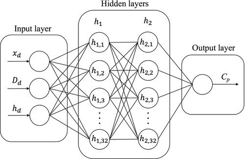
Figure 6 graphically illustrates the setting of the ANN constructed in the current paper. The ANN with two hidden layers where each of the layers has 32 neurons is applied to construct the surrogate model. The three dimple's parameters are inputs of the ANN and the power coefficient is the output. As the activation function, the rectified linear unit (ReLu) function is used. The regulation parameter and learning rate used in the current paper are ${10}^{-4}$ and 0.01, respectively. Constructing the surrogate modeling with the ANN is performed using the open-source library TensorFlow (Abadi et al., 2016).

Figure 6. The graphical description for the settings of the ANN. The three design parameters are trained using the ANN with two-hidden layers of 32 neurons each. The output of the ANN is set as the power coefficient.

4.4. Design exploration

After the surrogate model has been constructed, an optimal set of design parameters maximizing the power coefficient should be found. To successfully implement this task, a good searching method that can find a global (not local) optimum set should be used. The searching method used in the current paper is the genetic algorithm, which finds an optimal solution by mimicking the phenomenon of natural evolution. Unlike the gradient-based searching algorithms such as the steepest descent method and conjugate gradient method that easily converge to the local minimum solution (Shewchuk, 1994), the genetic algorithm does not use gradient information to search for the solution. Rather, it is a stochastic way of finding the optimal design parameters that are more likely to find the global minimum value. Once the initial populations of the sets of the design parameters are randomly created, the genetic algorithm starts the evolution process, including crossover, mutation and selection in the population pool to make the design parameters evolve over generations (Whitley, 1994). This evolution process is repeated until the maximum number of generations is reached or the change of the fitness value is smaller enough for the population. The population size and mutation rate of the genetic algorithm used in the current study are 50 and 0.01, respectively.

5. Results

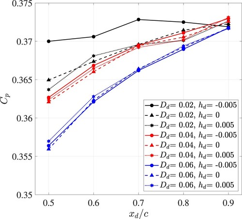
Figure 7 presents the distribution of the power coefficients of the 45 design points in the design of experiment step as a function of the three design parameters used in the current paper. In all cases, the wind turbines with dimples show better performance than the reference wind turbine, in which the power coefficient is approximately 0.352. For most $x_d$, the dimples with $D_d=0.02c$ and $h_d=-0.005c$ show the highest power coefficients when compared with the other cases. As the value of $x_d$ increases, meaning that the dimple approaches the trailing edge of the wind turbine blade, the power coefficient increases, regardless of the values of $D_d$ and $h_d$, except for the case when $D_d=0.02c$ and $h_d=-0.005c$, whose maximum power coefficient is measured at $x_d=0.7c$. In addition, as $x_d$ increases, the power coefficient is less sensitive to $D_d$ and $h_d$, which indicates that the influence of dimple's size and depth on the power coefficient diminishes as the dimple approaches the trailing edge. Furthermore, high power coefficient is identified when a dimple is small for most $x_d$ and the power coefficient more sensitively changes as a function of $x_d$ when the dimple is large ($D_d=0.06c$) than when it is small ($D_d=0.02c$ and $D_d=0.04c$). Among the dimples located along the same horizontal position, the influence of $h_d$ on the power coefficient is more clearly identified when the dimple is small ($D_d=0.02c$) than when it is large ($D_d=0.04c$ and $D_d=0.06c$).

Figure 7. Power coefficients of the 45 design points in the design of experiment.

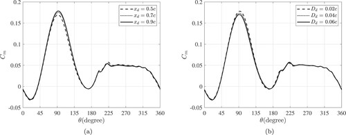
To identify the effects of the dimple's position, the moment coefficients of the three wind turbines where each one has the differently located but same-size ($D_d=0.06c$, $h_d=0$) semicircular dimples on the lower surface are presented in Figure 8(a). The difference of the moment coefficient with respect to the azimuthal angle for these three turbines are mostly shown at the upwind and downwind paths, while the difference is not clearly observed in the leeward and windward paths. This supports the fact that the physical phenomenon happens at the usual wind turbine: most of the torque rotating the wind turbine arises in the upwind and downwind paths so that the performance of the wind turbine can be roughly evaluated by identifying the distribution of the moment coefficient only in the upwind and downwind paths. One interesting point here is the opposite variation of the moment coefficient at the two paths with respect to $x_d$. As $x_d$ increases, the moment coefficient increases in the upwind path (especially around $\theta ={90}^{\circ }$), but a slight decrease of the moment coefficient is observed in the downwind path. The amount of increment of the moment coefficient in the upwind path is higher than its decrease in the downwind path, consequently making the rise of the power coefficient of the wind turbine with the dimple close to the trailing edge. When the moment coefficients of the wind turbines with the dimples created at the same $x_d$ and $h_d$ are compared, a similar phenomenon is found as $D_h$ reduces (see Figure 8(b)).

Figure 8. The moment coefficients of the three turbines with the differently located but same-size ($D_d=0.06c$, $h_d=0$) semicircular dimples are presented in (a). The same graph is presented in (b) but for the three wind turbines with the dimples created at the same $x_d$ and $h_d$ in which the values are $x_d=0.5c$ and $h_d=-0.005c$.

After figuring out the influences of the three dimple's parameters on the performance of the wind turbine, optimization is carried out with the parameters to search for the configuration of a dimple maximizing the wind turbine's performance. To prevent the genetic algorithm from finding a huge dimple that can make the wind turbine fragile, one constraint considered in the current paper is (16) $\frac{D_d/2+h_d}{t(x_d)}\le \gamma ,$(16) where γ is the constant defined by users and $t(x_d)$ is the thickness of the reference wind turbine airfoil at $x=x_d$. Because the numerator in Equation (16(16) $\frac{D_d/2+h_d}{t(x_d)}\le \gamma ,$(16) ) indicates the depth of the dimple at $x=x_d$, the left hand side of the equation implies the ratio of the dimple's depth regarding the reference airfoil's thickness at the center of the dimple. In the present study, γ is set to 0.5, assigning the constraint that the depth of the dimple cannot exceed half of the reference airfoil's thickness at the center.

From the results of the design of experiment, the power coefficient of the wind turbine with the dimple increases as the dimple approaches the trailing edge of the blade. Based on this, the upper limit of the design parameter $x_d$ is extended from 0.9c to 0.95c with the expectation that the dimple showing a higher power coefficient can be explored. Expanding the ranges of the design parameters after the design of experiment makes the ANN predict the power coefficient in the sense of extrapolation, but the ANN can provide a reasonable prediction accuracy even under this circumstance (Oh et al., 2017).

The optimization process used in the current paper is as follows: First, the 45 initial design points for the design of experiment are distributed in the design space. Next, each of wind turbines defined by the 45 design points is created, and their power coefficients are calculated by simulating the flow around them. Once the power coefficient is calculated, the ANN is trained with the dataset to construct a surrogate model for predicting the power coefficient with respect to the design parameters. The genetic algorithm searches for an optimal set of design parameters, which is expected to create an optimal wind turbine, and then, the actual power coefficient of the optimal wind turbine is computed using the CFD. After that, the ANN is retrained by adding the optimal set of design parameters with its CFD-computed power coefficient to the dataset, and the surrogate model is reconstructed using the most recent ANN. The genetic algorithm searches for a new optimal set of design parameters, and the process keeps continuing in this fashion. This loop is repeated until the maximum optimization iteration (defined here as 5) has been reached.

At all ANNs constructed during the optimization loop in the current study, both the training and test errors, which are defined as the root-mean-square deviation between the power coefficients computed from the ANN and CFD, are less than ${10}^{-3}$, which shows the ANNs' good prediction accuracy. The ANN-based optimization method in the current study finds the optimal set of the design parameters at at $x_d=0.95c$, $D_d=0.02c$ and $h_d=-0.0049c$. Mounting this optimal dimple on the reference wind turbine makes the power coefficient increase by approximately 6.46$\mathrm{\%}$ at $\lambda =2.5$. The wind turbine mounting this optimal dimple will be referred to as the optimal wind turbine in the rest of the paper.

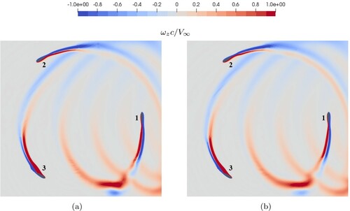
The contours of the instantaneous nondimensionalized z-vorticity at the reference and optimal wind turbines are shown in Figure 9. For each case, three turbine blades are marked as 1, 2 and 3 to visualize them clearly in the figure. The contours presented in Figure 9 are the moment when the azimuthal angle is $\theta ={270}^{\circ }$ with respect to turbine blade 1. In both cases, when blades 2 and 3 are compared, the trace of the blade wake is long and thick at blade 3, which means that the wake grows behind the blade as the wind turbine rotates in the upwind and leeward paths. Then, as the blade continues to rotate, the blade wake is shedded downstream in the downwind path.

Figure 9. Contours of the instantaneous nondimensionalized z-vorticity. (a) reference wind turbine (b) optimal wind turbine.

The moment coefficients of the reference and optimal wind turbines for the last turbine revolution are presented in Figure 10. In the upwind path, the most distinguishable discrepancy between the two turbines are identified approximately around ${85}^{\circ }\le \theta \le {135}^{\circ }$. In this range, the peak of the moment coefficient of the optimal wind turbine is not only higher compared with the reference wind turbine, but the peak is also observed approximately 2 degrees later, which seems to be related to the delay of the flow separation for the optimal wind turbine (see Figure 11 for more detail). For most of the downwind path, the moment coefficient of the optimal wind turbine is better than the reference wind turbine's one. It is believed that the reduction of the blade wake at the optimal wind turbine during the downwind path appears as the rise of the moment coefficient in the corresponding region.

Figure 10. Comparison of the moment coefficients for the last turbine revolution of the reference and optimal wind turbines. The red box in (a) is enlarged in (b).

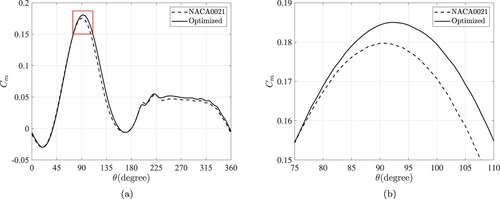
Figure 11. Streamlines around the reference and optimal wind turbines.

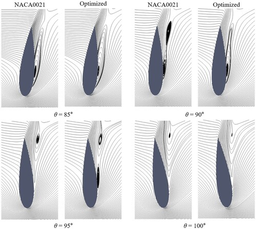
Figure 11 shows the streamlines around the reference and optimal wind turbines when they are located from $\theta ={85}^{\circ }$ to $\theta ={100}^{\circ }$. In each case, as the azimuthal angle increases, the vortex existing on the suction side of the wind turbine breaks into the two vortices where the primary vortex (existing close to the leading edge) is reattached to the surface of the wind turbine, while the secondary vortex (existing close to the trailing edge) dissipates around the trailing edge. From the figure, it is possible to see that the leading edge vortex in the reference case breaks up earlier compared with the optimal wind turbine case. The vortex formed on the surface of the reference wind turbine at $\theta ={85}^{\circ }$ starts to separate as the turbine rotates further, and two distinguishable vortices are seen at $\theta ={90}^{\circ }$, where the secondary vortex is about to shed from the primary vortex. However, at the optimal wind turbine, the apparent primary and secondary vortices are first detected at $\theta ={95}^{\circ }$, implying the separation arises between $\theta ={90}^{\circ }$ and $\theta ={95}^{\circ }$. The authors' further investigation finds that the separation in the optimal case occurs approximately 2 degrees later than the reference case, which is the same amount of delay that was identified at the peak points of the moment coefficients between the reference and optimal wind turbines. This is because the lift force over the airfoil rapidly decreases due to flow separation (Carr, 1988; Choudhry et al., 2014), and therefore, the fact that the flow separation of the reference wind turbine occurs 2 degrees earlier than the optimal one indicates that the rapid reduction of the lift force over the blade (causing a sudden decrease of the moment coefficient) arises with the same amount of degrees as earlier in the reference wind turbine. In other words, the dimple mounted on the surface of the optimal wind turbine causes a flow separation delay, and it makes the optimal wind turbine generate a higher lift force than the reference one, which appears as the increment of the power coefficient of the optimal wind turbine.

The performance of the optimal wind turbine is evaluated at different tip speed ratios to test its performance besides the tip speed ratio where it is optimized ($\lambda =2.5$). As shown in Figure 12, the increment of the power coefficients of the optimal wind turbine with respect to the reference wind turbine decreases as the tip speed ratio spreads out from $\lambda =2.5$, but the optimal wind turbine performs better than the reference one for all the test cases. The moment coefficients of the reference and optimal wind turbines as a function of the tip speed ratio are presented as contour plots in Figure 13(a,b), respectively, where the color indicates the values of the moment coefficients. Figure 13(c) shows the difference of the moment coefficient between the two wind turbines where a positive value means the moment coefficient of the optimal wind turbine is higher than the reference one. For both turbines, the maximum moment coefficients are shown around $\theta ={90}^{\circ }$, but the azimuthal angles when the moment coefficients are at their peak increase as the tip speed ratio rises. At high tip speed ratios, the moment coefficients of the optimal wind turbine are a bit uniformly higher than the reference ones. However, when the tip speed ratio is low, two apparent positive and negative regions are observed.

Figure 12. The power coefficients of the reference and optimal wind turbines are compared as a function of the tip speed ratio. Note that optimal wind turbine in this study is obtained at $\lambda =2.5$.

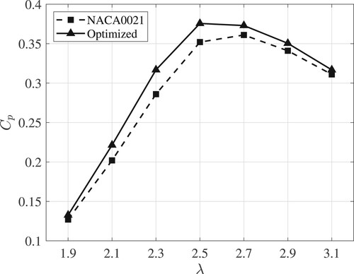
Figure 13. Contours of the moment coefficients of the reference and optimal wind turbines during the last turbine revolution are, repsectively, presented in (a) and (b) for different λ. The contour plotted in (c) shows the difference of the moment coefficient between the reference and optimal wind turbines where a positive number indicates a high moment coefficient of the optimal wind turbine.

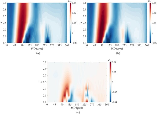
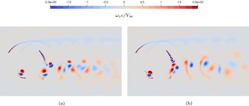
Figure 14 illustrates the contours of the instantaneous nondimensionalized z-vorticity at the reference and optimal wind turbines at $\lambda =1.9$. At both wind turbines, more distinct vortex shedding is observed than the one shown at $\lambda =2.5$. This is a natural phenomenon because a blade in a pitching motion at a low tip speed ratio experiences a wide variation regarding its angle of attack, and therefore, a dynamic stall more actively occurs on the blade operating at a low tip speed ratio. When the nondimensionalized z-vorticity contours at two wind turbines are compared, the vortices shedding from the reference turbine is stronger and last longer than the ones from the optimal wind turbine. When these persistent shed vortices meet another blade installed near the wake region, the pressure distribution on the blade will fluctuate, which can cause blade vibrations, noise increases and a deterioration of the turbine's performance.

Figure 14. Contours of the instantaneous nondimensionalized z-vorticity at $\lambda =1.9$. (a) reference wind turbine (b) optimal wind turbine.

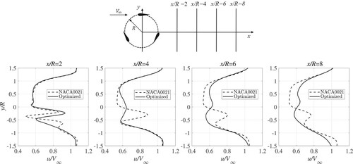
At $\lambda =1.9$, the streamwise direction time-averaged nondimensionalized velocities of the reference and optimal wind turbines are presented in Figure 15 at different downstream locations. Apparent discrepancies between the two wind turbines are shown at $-1<y/R<0$ due to the difference of the dissipation features of the shed vortices. The oscillation of the time-averaged nondimensionalized velocity, which is caused by the presence of the shed vortices, is not only small and narrow, but it also disappears quickly in the optimal case. This indicates that the vortices shed from the optimal wind turbine blades are weaker, distribute more locally and decay faster than the ones detached from the reference wind turbine blades, which supports the interpretation deduced from Figure 14.

Figure 15. The time-averaged (for last turbine revolution) nondimensionalized streamwise velocity of the reference and optimal wind turbines at $\lambda =1.9$. The data here are sampled at four different locations ($x/R=2,4,6$ and 8).

6. Conclusions

6.1. Summary

In the present study, the CFD simulations and optimization are carried out for a H-Darrieus VAWT with a dimple to investigate the effects of the dimple's configuration on the performance of the VAWT and to find the optimal configuration of a dimple maximizing its performance. The three-bladed NACA0021 wind turbine is chosen as the reference wind turbine and a dimple is mounted on the lower surface of each blade. To change the configuration of a dimple, the three parameters varying the dimple's position, size and depth are used. With these parameters, the optimization is performed at $\lambda =2.5$ using the ANN and genetic algorithm. After the aerodynamic properties of various wind turbines with dimples were investigated, the following conclusions are deduced:

• Among the parameters to control the configuration of a dimple, the dimple's position parameter most significantly affects the wind turbine's performance. As the position of the dimple approaches the trailing edge, the power coefficient of the wind turbine increases. From the dimple circle's diameter, which controls the size of the dimple, the smaller the diameter is, the higher the power coefficient will be obtained in the most cases, but this attribute becomes weaker as the dimple approaches the trailing edge. For the dimple's depth parameter, a change of the power coefficient is observed more clearly when the dimple size is small than when it is large.

• As a result of this optimization, the optimal configuration of a dimple showing approximately $6.46\mathrm{\%}$ performance improvement with respect to the reference wind turbine is found. When the flows around the reference and optimal wind turbine blades are compared, a reduction of the blade wake and delay of the flow separation are observed in the optimal case, which makes the optimal wind turbine better than the reference one.

• When the optimal wind turbine obtained at $\lambda =2.5$ is simulated at other tip speed ratios, the power coefficient of the optimal wind turbine is still higher than the reference wind turbine's power coefficient. However, the increment of the power coefficient is reduced as the tip speed ratio moves away from $\lambda =2.5$. When the flows of the reference and optimal wind turbines are investigated at $\lambda =1.9$, the shed vortices from the optimal wind turbine blade are weaker and decay faster than the ones shed from the reference blade. These flow characteristics indicate that the shed vortices produced by the optimal wind turbine less negatively affect the other wind turbines installed inside the wake region, which can be a significant advantage when the wind turbines are installed in an array.

6.2. Discussion

All dimples in the current study are placed on the particular wind turbine airfoil (NACA0021). Because of this restriction, it is not clearly investigated whether the physical observations made in the current study are also maintained when the wind turbine airfoil contour is modified. However, when the authors implement the flow simulation with a different wind turbine airfoil (NACA0015), the physical phenomenons observed with the NACA0021 wind turbine airfoil can still be identified. For example, a NACA0015 wind turbine with a 0.04c diameter semicircular dimple placed at x = 0.9c shows a flow separation delay compared with the NACA0015 wind turbine without a dimple. Not only that, but the wind turbine's performance is improved more when the dimple is created near the trailing edge and when the dimple size is small, which completely follows the observations made with dimple-equipped NACA0021 wind turbines and shows the expandability of the important findings of the current study. All simulation results conducted with the NACA0015 wind turbines are presented in Table 3.

Table 3. The power coefficients of the NACA0015 wind turbines with various dimples.

$x_d$	$D_d$	$C_p$
0.5c	0.02c	0.371
0.5c	0.04c	0.369
0.5c	0.06c	0.364
0.7c	0.04c	0.373
0.9c	0.04c	0.376

Note: For all wind turbines, the parameter $h_d$ is set to zero.

In addition, wind turbine simulations in the current study are carried out at the fixed pitching angle (when it is zero). However, the authors strongly believe that the performance of the wind turbine with a dimple will change as a function of the pitching angle and its performance can be intensified more by controlling the pitching angle properly. As a future work, the effects of the wind turbine's dimple will be analyzed by modifying the pitching angle, and its contribution will be investigated.

Nomenclature

a	=	Axial induction factor [-]
A	=	Turbine swept area [${\mathrm{m}}^2$]
c	=	Blade chord length [m]
$C_d$	=	Drag coefficient [-]
$C_l$	=	Lift coefficient [-]
$C_m$	=	Moment coefficient [-]
$C_n$	=	Normal force coefficient [-]
$C_t$	=	Tangential force coefficient [-]
$C_p$	=	Power coefficient [-]
${\hat{C}}_p$	=	Power coefficient computed with ANN [-]
D	=	Turbine diameter [m]
$D_d$	=	Dimple diameter [%c]
$F_t$	=	Tangential force [N]
${\overline{F}}_t$	=	Average tangential force [N]
$h_d$	=	Dimple depth [%c]
H	=	Turbine height [m]
M	=	Torque [$\mathrm{N}\cdot \mathrm{m}$]
Q	=	Total torque [$\mathrm{N}\cdot \mathrm{m}$]
R	=	Turbine radius [m]
$R{e}_c$	=	Blade chord-based Reynolds number ($c{V}_{\mathrm{\infty }}\sqrt{1+{\lambda }^2}/\nu$)[-]
$V_a$	=	Axial flow velocity [m/s]
$V_{\mathrm{\infty }}$	=	Freestream velocity [m/s]
$V_{\theta }$	=	Tangential velocity [m/s]
W	=	Relative wind velocity [m/s]
$x_d$	=	Dimple position [%c]
α	=	Angle of attack [deg]
γ	=	Constraint constant [-]
θ	=	Azimuthal angle [deg]
κ	=	Regularization factor [-]
λ	=	Tip speed ratio [-]
ν	=	Air kinematic viscosity [m${}^2$/s]
ρ	=	Air density [$\mathrm{kg}/{\mathrm{m}}^3$]
ω	=	Turbine angular velocity [rad/s]
${\omega }_z$	=	z-directional angular velocity [rad/s]
$\mathbf{w}$	=	Weight vector[-]
L	=	Loss function [-]

Disclosure statement

No potential conflict of interest was reported by the author(s).

Additional information

Funding

This work was supported by the National Research Foundation of Korea (NRF) grant funded by the Korea government (MSIT) (No. 2019K1A3A1A80113330).

References

- Abadi M., Barham P., Chen J., Chen Z., Davis A., Dean J., Devin M., Ghemawat S., Irving G., Isard M., Kudlur M., Levenberg J., Monga R., Moore S., Murray D. G., Steiner B., Tucker P., Vasudevan V., Warden P.,…Zheng X. (2016). TensorFlow: A System for Large-Scale Machine Learning. 12th USENIX Symposium on Operating Systems Design and Implementation (OSDI ’16).
- Akansu S. O., Dagdevir T., & Kahraman N. (2017). Numerical investigation of the effect of blade airfoils on a vertical axis wind turbine. Isı Bilimi ve Tekniği Dergisi, 38(1), 115–125.
- Balduzzi F., Bianchini A., Carnevale E. A., Ferrari L., & Magnani S. (2012). Feasibility analysis of a Darrieus vertical-axis wind turbine installation in the rooftop of a building. Applied Energy, 97, 921–929. https://doi.org/https://doi.org/10.1016/j.apenergy.2011.12.008
- Bani-Hani E. H., Sedaghat A., AL-Shemmary M., Hussain A., Alshaieb A., & Kakoli H. (2018). Feasibility of highway energy harvesting using a vertical axis wind turbine. Energy Engineering, 115(2), 61–74. https://doi.org/https://doi.org/10.1080/01998595.2018.11969276
- Beri H., & Yao Y. (2011). Double multiple streamtube model and numerical analysis of vertical axis wind turbine. Energy and Power Engineering, 3(3), 262. https://doi.org/https://doi.org/10.4236/epe.2011.33033
- Brownlee B. G. (1988). A vortex model for the vertical axis wind turbine [Unpublished doctoral dissertation]. Texas Tech University.
- Carr L. W. (1988). Progress in analysis and prediction of dynamic stall. Journal of Aircraft, 25(1), 6–17. https://doi.org/https://doi.org/10.2514/3.45534
- Castelli M. R., Englaro A., & Benini E. (2011). The Darrieus wind turbine: Proposal for a new performance prediction model based on CFD. Energy, 36(8), 4919–4934. https://doi.org/https://doi.org/10.1016/j.energy.2011.05.036
- Chong W., Pan K., Poh S., Fazlizan A., Oon C., Badarudin A., & Nik-Ghazali N. (2013). Performance investigation of a power augmented vertical axis wind turbine for urban high-rise application. Renewable Energy, 51, 388–397. https://doi.org/https://doi.org/10.1016/j.renene.2012.09.033
- Choudhry A., Arjomandi M., & Kelso R.. (2014). Lift curve breakdown for airfoil undergoing dynamic stall. In Proceedings of the 19th australasian fluid mechanics conference, Melbourne, Australia.
- DuMouchel W., & Jones B. (1994). A simple Bayesian modification of D-optimal designs to reduce dependence on an assumed model. Technometrics, 36(1), 37–47. https://doi.org/https://doi.org/10.1080/00401706.1994.10485399
- Durakovic B. (2017). Design of experiments application, concepts, examples: State of the art. Periodicals of Engineering and Natural Sciences, 5(3), 421–439. https://doi.org/https://doi.org/10.21533/pen.v5i3.145
- Eriksson S., Bernhoff H., & Leijon M. (2008). Evaluation of different turbine concepts for wind power. Renewable and Sustainable Energy Reviews, 12(5), 1419–1434. https://doi.org/https://doi.org/10.1016/j.rser.2006.05.017
- Ez Abadi A. M., Sadi M., Farzaneh-Gord M., Ahmadi M. H., Kumar R., & Chau K. w. (2020). A numerical and experimental study on the energy efficiency of a regenerative heat and mass exchanger utilizing the counter-flow Maisotsenko cycle. Engineering Applications of Computational Fluid Mechanics, 14(1), 1–12. https://doi.org/https://doi.org/10.1080/19942060.2019.1617193
- Ferreira C. S., Van Kuik G., Van Bussel G., & Scarano F. (2009). Visualization by PIV of dynamic stall on a vertical axis wind turbine. Experiments in Fluids, 46(1), 97–108. https://doi.org/https://doi.org/10.1007/s00348-008-0543-z
- Ghalandari M., Ziamolki A., Mosavi A., Shamshirband S., Chau K. W., & Bornassi S. (2019). Aeromechanical optimization of first row compressor test stand blades using a hybrid machine learning model of genetic algorithm, artificial neural networks and design of experiments. Engineering Applications of Computational Fluid Mechanics, 13(1), 892–904. https://doi.org/https://doi.org/10.1080/19942060.2019.1649196
- Giorgetti S., Pellegrini G., & Zanforlin S. (2015). CFD investigation on the aerodynamic interferences between medium-solidity Darrieus vertical axis wind turbines. Energy Procedia, 81, 227–239. https://doi.org/https://doi.org/10.1016/j.egypro.2015.12.089
- Greenshields C. J. (2015). OpenFOAM user guide (version, 3(1), 47). OpenFOAM Foundation Ltd.
- Ismail M. F., & Vijayaraghavan K. (2015). The effects of aerofoil profile modification on a vertical axis wind turbine performance. Energy, 80, 20–31. https://doi.org/https://doi.org/10.1016/j.energy.2014.11.034
- Jouhaud J. C., Sagaut P., Montagnac M., & Laurenceau J. (2007). A surrogate-model based multidisciplinary shape optimization method with application to a 2D subsonic airfoil. Computers & Fluids, 36(3), 520–529. https://doi.org/https://doi.org/10.1016/j.compfluid.2006.04.001
- Kang D. H., Shin W. S., & J. H. Lee (2014, December). Experimental study on the performance of urban small vertical wind turbine with different types. Journal of Fluid Machinery, 17(6), 64–68. https://doi.org/https://doi.org/10.5293/kfma.2014.17.6.064
- Kuram E., Ozcelik B., Bayramoglu M., Demirbas E., & Simsek B. T. (2013). Optimization of cutting fluids and cutting parameters during end milling by using D-optimal design of experiments. Journal of Cleaner Production, 42, 159–166. https://doi.org/https://doi.org/10.1016/j.jclepro.2012.11.003
- Ma L., Wang X., Zhu J., & Kang S. (2019). Dynamic stall of a vertical-Axis wind turbine and its control using plasma actuation. Energies, 12(19), 3738. https://doi.org/https://doi.org/10.3390/en12193738
- McCroskey W. J. (1981). The phenomenon of dynamic stall (Tech. Rep.). National Aeronuatics and Space Administration Moffett Field Ca Ames Research…
- Mohammed A. A., Ouakad H. M., Sahin A. Z., & Bahaidarah H. (2019). Vertical axis wind turbine aerodynamics: summary and review of momentum models. Journal of Energy Resources Technology, 141(5), Article 050801. https://doi.org/https://doi.org/10.1115/1.4042643
- Moran J. (2003). An introduction to theoretical and computational aerodynamics. Courier Corporation.
- Oh S. (2020). Comparison of a response surface method and artificial neural network in predicting the aerodynamic performance of a wind turbine airfoil and its optimization. Applied Sciences, 10(18), 6277. https://doi.org/https://doi.org/10.3390/app10186277
- Oh S., Jiang C. H., Jiang C., & Marcus P. S. (2017). Finding the optimal shape of the leading-and-trailing car of a high-speed train using design-by-morphing. Computational Mechanics, 62(1), 1–23. https://doi.org/https://doi.org/10.1007/s00466-017-1482-4
- Olsman W., & Colonius T. (2011). Numerical simulation of flow over an airfoil with a cavity. AIAA Journal, 49(1), 143–149. https://doi.org/https://doi.org/10.2514/1.J050542
- Qamar S. B., & Janajreh I. (2017). Investigation of effect of cambered blades on Darrieus VAWTs. Energy Procedia, 105, 537–543. https://doi.org/https://doi.org/10.1016/j.egypro.2017.03.353
- Riegler H. (2003). HAWT versus VAWT: Small VAWTs find a clear niche. Refocus, 4(4), 44–46. https://doi.org/https://doi.org/10.1016/S1471-0846(03)00433-5
- Scheurich F., Fletcher T. M., & Brown R. E. (2011). Simulating the aerodynamic performance and wake dynamics of a vertical-axis wind turbine. Wind Energy, 14(2), 159–177. https://doi.org/https://doi.org/10.1002/we.v14.2
- Seng S., Monroy C., & Malenica Š.. (2017)). On the use of Euler and Crank-Nicolson time-stepping schemes for seakeeping simulations in OpenFOAM . In VII International conference on computational methods in marine engineering.
- Shewchuk J. R. (1994). An introduction to the conjugate gradient method without the agonizing pain. Carnegie-Mellon University, Department of Computer Science.
- Simão Ferreira C. (2009). The near wake of the VAWT: 2D and 3D views of the VAWT aerodynamics.
- Sobhani E., Ghaffari M., & Maghrebi M. J. (2017). Numerical investigation of dimple effects on darrieus vertical axis wind turbine. Energy, 133, 231–241. https://doi.org/https://doi.org/10.1016/j.energy.2017.05.105
- Tian W., Mao Z., An X., Zhang B., & Wen H. (2017). Numerical study of energy recovery from the wakes of moving vehicles on highways by using a vertical axis wind turbine. Energy, 141, 715–728. https://doi.org/https://doi.org/10.1016/j.energy.2017.07.172
- Tirkey A., Sarthi Y., Patel K., Sharma R., & Sen P. K. (2014). Study on the effect of blade profile, number of blade, Reynolds number, aspect ratio on the performance of vertical axis wind turbine. International Journal of Science, Engineering and Technology Research (IJSETR), 3(12), 3183–3187.
- Tjiu W., Marnoto T., Mat S., Ruslan M. H., & Sopian K. (2015). Darrieus vertical axis wind turbine for power generation I: Assessment of Darrieus VAWT configurations. Renewable Energy, 75, 50–67. https://doi.org/https://doi.org/10.1016/j.renene.2014.09.038
- Viana F. A., Venter G., & Balabanov V. (2010). An algorithm for fast optimal Latin hypercube design of experiments. International Journal for Numerical Methods in Engineering, 82(2), 135–156. https://doi.org/https://doi.org/10.1002/nme.2750
- Vicente G., Coteron A., Martinez M., & Aracil J. (1998). Application of the factorial design of experiments and response surface methodology to optimize biodiesel production. Industrial Crops and Products, 8(1), 29–35. https://doi.org/https://doi.org/10.1016/S0926-6690(97)10003-6
- Whitley D. (1994). A genetic algorithm tutorial. Statistics and Computing, 4(2), 65–85. https://doi.org/https://doi.org/10.1007/BF00175354
- Youssefi S., Emam-Djomeh Z., & Mousavi S. (2009). Comparison of artificial neural network (ANN) and response surface methodology (RSM) in the prediction of quality parameters of spray-dried pomegranate juice. Drying Technology, 27(7–8), 910–917. https://doi.org/https://doi.org/10.1080/07373930902988247
- Zhao Z., Su D., Wang T., Xu B., Wu H., & Zheng Y. (2019). A blade pitching approach for vertical axis wind turbines based on the free vortex method. Journal of Renewable and Sustainable Energy, 11(5), Article 053301. https://doi.org/https://doi.org/10.1063/1.5099411
- Zhu H., Hao W., Li C., & Ding Q. (2019). Numerical study of effect of solidity on vertical axis wind turbine with Gurney flap. Journal of Wind Engineering and Industrial Aerodynamics, 186, 17–31. https://doi.org/https://doi.org/10.1016/j.jweia.2018.12.016