Numerical investigation on the scale-up rules of a supercritical water fluidized bed reactor using the two-fluid model

Abstract

The supercritical water fluidized bed reactor (SCWFBR) is a novel hydrogen production technique, so the understanding on its scale-up is limited. In this regard, the trial-and-error procedure is not an option for traditional experimental research because it is costly and high risk. To overcome these problems, numerical simulations were carried out in this study based on the two-fluid model (TFM) to examine the capability of different scale-up rules for the SCWFBR. The numerical model was first validated based on experimental results. Then, four different-sized SCWFBRs were designed, in which numerical simulations for both air–solid and supercritical water (SCW)–solid systems were conducted following different scale-up rules. The distributions of solid volume fraction, solid velocity and pressure in these reactors were fully investigated. Comparisons among the numerical results showed that keeping the Reynolds number, Froude number and dimensional inlet velocity constant is critical for the scale-up of both SCWFBRs and traditional gas–solid fluidized bed reactors (FBRs). Moreover, keeping the particle diameter constant is helpful in obtaining the similarity of the multiphase flow behavior. For the SCWFBR, but not for the traditional gas–solid FBR, a constant density ratio between solid and fluid should be kept during the scale-up. Finally, for the SCW–solid system with more active particle motions, the effect of the interparticle collisions should be considered in the scaling parameters at high Reynolds numbers.

KEYWORDS:

• Numerical simulation
• scale-up
• supercritical water
• fluidized bed reactor
• two-fluid model

1. Introduction

1.1. Background

The problem of global warming and depletion of traditional fossil sources is becoming more and more critical. In this scenario, the clean and efficient use of coal resources and further development of low-cost technologies for large-scale utilization of biomass energy are drawing tremendous attention from researchers worldwide. Hydrogen production based on supercritical water (SCW) is one of the most promising techniques in this regard (Correa & Kruse, 2017; Lu et al., 2011; Okolie et al., 2019). The main idea behind this technique is simply to put coal or/and biomass materials in a reactor filled with SCW, and hydrogen is produced through the chemical reaction between the solid materials and the SCW. Hydrogen energy is extremely clean to use and quite stable during transportation. Moreover, unlike traditional thermochemical conversion processes based on the combustion of biomass and coal in air, the SCW-based technique holds many advantages, such as direct gasification of lignite or wet biomass and efficient heating of bed materials. Most importantly, during the SCW-based hydrogen production process, those harmful nitrogen- and oxygen-containing contaminants are eliminated in the liquid phase as slags. In this way, nearly zero emissions of nitrogen oxides, sulfur oxides and solid particulate matters to the open air can be achieved. All of these advantages will make SCW-based hydrogen production one of the core techniques in the field of pollution-free conversion and utilization of clean energy in the coming decades.

During the SCW-based hydrogen production process, the mixing of the multiphase flow is achieved by the introduction of SCW through the solid materials, which takes place in a supercritical water fluidized bed reactor (SCWFBR). Previous studies have indicated that the hydrogen production rate essentially relies on the multiphase flow pattern in the reactor (Correa & Kruse, 2017; Lu et al., 2011; Okolie et al., 2019). Great efforts have been thus made to obtain the optimal flow pattern by laboratory experiments, according to the highest hydrogen production rate. Unfortunately, it is extremely hard to maintain this optimal flow in industrial reactors owing to the insufficient understanding of multiphase flow characteristics and scale-up rules. There is a huge risk in thoughtlessly scaling up the engineering reactors from a laboratory scale to an industrial size, which may have disastrous consequences. This is especially true for a time-consuming and expensive installation such as the SCWFBR, working in conditions of high pressure and temperature. In reality, traditional experimental measurements have great difficulty in providing comprehensive information for the scale-up of SCWFBRs. The current study aims to adopt numerical simulation as an alternative tool to investigate the spatial and temporal distribution of the multiphase flow in different-sized SCWFBRs, and to highlight the influences of the reactor structure and operating parameters. Optimization and scale-up of the SCWFBR can be thus achieved without large investments.

1.2. Previous work

In recent decades, the SCWFBR has been widely used for hydrogen production because it can overcome the drawback of plugging in tubular reactors (Lu et al., 2013; Matsumura & Minowa, 2004) and also because it exhibits higher gasification efficiency. Numerical simulations have played a vital role in the study of SCWFBR because the limitation of physical experimental measurement can be broken and more light can be shed on the complex process. Compared with the high investment in physical experiments, computer modeling is a much cheaper way to quantify the influence of various key operation parameters. Moreover, numerical simulations are helpful for understanding the mechanism of interaction between solids and SCW. Among various numerical schemes, the two-fluid model (TFM) is favored for solving actual engineering problems owing to its superiority in computational efficiency. For example, Wei et al. (2013) carried out TFM simulations to determine the optimal feeding methods and feeding rates of solid materials into the SCWFBR by examining their effects on solid distribution and residence time distribution. Lu, Wei, et al. (2015) established a novel TFM via a non-spherical particle drag model and adopted it to simulate the SCWFBR. A pseudo-homogeneous bed expansion between the classically bubbling and homogeneous fluidization was innovatively observed based on their numerical results. Lu et al. (2016) also adopted a TFM to investigate the SCWFBR and traditional gas–solid fluidized bed reactor (FBR) with an immersed tube. It was found that a high particle concentration could enhance the heat transfer coefficient around the tube in the traditional gas–solid FBR, but the opposite effects were observed for the SCWFBR. Based on the numerical results of the TFM, Ren et al. (2020) found that the increase in temperature can improve heterogeneous flow structure in the SCWFBR, especially in particle-dilute flow. Yao and Lu (2017) carried out TFM simulations to investigate the effects of operation conditions and reactor structure on gas yield and residence time, and explored the optimal operation rules for increasing gas yield.

Almost all of the aforementioned studies focused on the laboratory-scale SCWFBR. However, it is questionable to directly apply the knowledge obtained from laboratory-scale reactors to design a full-scale installation. This is because the multiphase flow can show completely different behavior in different-sized reactors, even though they have geometric similarity. For example, the increase in the reactor size can cause an increase in the bubble rising velocity (Matsen, 1996) and the enhancement of solid mixing and diffusion (Bashiri et al., 2010) owing to the decrease in the boundary wall effect (Werther, 1974). Complicating the problem is the art of scale-up, which is still subject to many uncertainties and pitfalls (Rüdisüli et al., 2012). As mentioned by Matsen (1997): ‘Scale-up is not an exact science, but is rather that mix of physics, mathematics, witchcraft, history and common sense that we call engineering’. For the scale-up of traditional gas–solid FBRs, Knowlton et al. (2005) claimed that the optimum type of hydrodynamic fluid/solid contacting mode must be determined and maintained during the scale-up. Knowlton et al. (2005) also confirmed the importance of numerical simulation in predicting the effect of reactor size on the multiphase hydrodynamics. The intuitive rule to guide the scale-up is to utilize one or a group of scaling parameters regardless of reactor size. By doing so, the multiphase flow, although in different-sized reactors, should show similar behavior, as long as those dimensionless scaling parameters are not varied. This kind of scaling parameter has been obtained from the non-dimensionalization of the mass and momentum balances and their boundary conditions by Glicksman (1984, 1988), Glicksman et al. (1993, 1994), Horio et al. (1986), Bricout and Louge (2004) and Bonniol et al. (2009). Their capability to guide the scale-up of traditional gas FBR has been examined by several other researchers. Based on TFM simulations, Ommen et al. (2006) argued that the full set (Glicksman, 1984) of scaling parameters provides the worst predictive results during the scale-up, while the simplified (Glicksman, 1988) and the extended sets perform better, but neither leads to complete similarity. In contrast, the TFM numerical results of Wang et al. (2009) and Wu et al. (2016) showed that the full set of scaling parameters (Glicksman, 1984) is competent in predicting the multiphase flow behavior and heat transfer when scaling up a jetting FBR. The Eulerian–Lagrangian numerical results of Maio and Renzo (2013) indicated that the full set of scaling parameters (Glicksman, 1984) produces scaled systems preserving the similitude for all scale factors, whereas the simplified set (Glicksman, 1988) does not. The latter is only valid for a scale factor of 2, while for a factor of 4 the similitude properties are lost. Maio and Renzo (2013) believed that the failure of the scaling rules is due to too many assumptions and simplifications being made. For example, it is common in the scaling rules to assume incompressible fluid and no interparticle collisions (Jong & Ommen, 2009) and to ignore surface forces on particles due to static charge (Kelkar & Ng, 2002). Ebrahimi et al. (2017) conducted Eulerian–Lagrangian simulations to fully examine the full set of scaling parameters (Glicksman, 1984) on a single-spout FBR, and found a very good overall hydrodynamic similarity for all of the test cases. A minor discrepancy observed between the base and scaled cases was explained through force analysis.

In addition to verifying the scaling parameters, numerical simulations were adopted to investigate the scale-up effect of various FBRs. Zhong et al. (2013) used the TFM to numerically study the minimum spouting velocity of scaled-up spouted beds. Verma et al. (2015) used the TFM to fully investigate the differences in bubble and solid flow characteristics among FBRs with different diameters. Lu et al. (2017) used the TFM to discuss the scale-up effects through simulations of a series of methanol-to-olefins (MTO) reactors of different sizes. These works again confirm that the TFM is a competent tool for investigating the scale-up of large-scale reactors.

1.3. Motivation for and summary of this work

A survey of the literature showed that previous research mainly focused on the scale-up of traditional gas FBR, whereas disagreement over the capability of different scale-up rules still exists. Furthermore, the question of whether those scale-up rules can be used to design an SCWFBR remains open. The numerical results of Lu, Huang, et al. (2015) showed that bubble dynamic characteristics in the SCWFBR differ significantly from those in traditional gas–solid FBRs. The aim of the current study is thus straightforward: to conduct numerical simulations to discuss the change in multiphase flow behavior during the scale-up and finally to determine a suitable scale-up rule for the SCWFBR. The determined scale-up rule could be directly adopted by other researchers to scale up their own reactors. The remainder of the paper is organized as follows. Section 2 introduces the numerical issues. Section 3 presents the validation of the TFM model. Section 4 reports the numerical results with corresponding discussion. Finally, conclusions are drawn in Section 5.

2. Governing equations and scaling-up methodology

2.1. Governing equations

The TFM (Boemer et al., 1998) treats both solid and fluid phases as interpenetrating continua, and the kinetic theory of granular flow is used for the closure of the solid stress term. The method has been successfully applied to simulate pressurized and SCWFBRs. The governing equations include conservation of mass, momentum and component transport equations, as shown in Table 1. The interaction between the fluid and solid phases is calculated using the Syamlal and O’Brien model (Syamlal & O’Brien, 1989).

Table 1. Governing equations of the two-fluid model (TFM).

Equations
Continuity equation
$\frac{\mathrm{\partial }}{\mathrm{\partial }t}\left({\alpha }_f{\rho }_f\right)+\mathrm{\nabla }\cdot \left({\alpha }_f{\rho }_f{\overrightarrow{v}}_f\right)=0$
$\frac{\mathrm{\partial }}{\mathrm{\partial }t}\left({\alpha }_s{\rho }_s\right)+\mathrm{\nabla }\cdot \left({\alpha }_s{\rho }_s{\overrightarrow{v}}_s\right)=0$
Momentum equation
$\frac{\mathrm{\partial }}{\mathrm{\partial }t}\left({\alpha }_f{\rho }_f{\overrightarrow{v}}_f\right)+\mathrm{\nabla }\cdot \left({\alpha }_f{\rho }_f{\overrightarrow{v}}_f{\overrightarrow{v}}_f\right)=-{\alpha }_f\mathrm{\nabla }p+\mathrm{\nabla }\cdot {\overline{\overline{\tau }}}_f+{\alpha }_f{\rho }_f\overrightarrow{g}+K_{fs}\left({\overrightarrow{v}}_s-{\overrightarrow{v}}_f\right)$
$\frac{\mathrm{\partial }}{\mathrm{\partial }t}\left({\alpha }_s{\rho }_s{\overrightarrow{v}}_s\right)+\mathrm{\nabla }\cdot \left({\alpha }_s{\rho }_s{\overrightarrow{v}}_s{\overrightarrow{v}}_s\right)=-{\alpha }_s\mathrm{\nabla }p-\mathrm{\nabla }{p}_s+\mathrm{\nabla }\cdot {\overline{\overline{\tau }}}_s+{\alpha }_f{\rho }_f\overrightarrow{g}+K_{fs}\left({\overrightarrow{v}}_f-{\overrightarrow{v}}_s\right)$
Solid fluctuation equation
$\frac{3}{2}\left[\frac{\mathrm{\partial }}{\mathrm{\partial }t}\left({\alpha }_s{\rho }_s{\mathrm{\Theta }}_s\right)+\mathrm{\nabla }\cdot \left({\alpha }_s{\rho }_s\overrightarrow{{\upsilon }_s}{\mathrm{\Theta }}_s\right)\right]=\left(-\mathrm{\nabla }{p}_s\overline{\overline{\mathrm{I}}}+{\overline{\overline{\tau }}}_s\right):\mathrm{\nabla }{\upsilon }_s+\mathrm{\nabla }\cdot \left(K_{\theta s}\mathrm{\nabla }{\mathrm{\Theta }}_s\right)-{\gamma }_{\mathrm{\Theta }s}$
Interphase exchange coefficients
$K_{fs}=\frac{3{\alpha }_s{\alpha }_f{\rho }_f}{4{{\nu }^2}_{r,s}{d}_s}{C}_D\left(\frac{R{e}_s}{{\nu }_{r,s}}\right)\left|{\overrightarrow{\nu }}_s-{\overrightarrow{\nu }}_f\right|$
$C_D={\left(0.63+\frac{4.8}{\sqrt{R{e}_s/{\nu }_{r,s}}}\right)}^2$
$R{e}_s=\frac{{\rho }_f{d}_s\left|{\overrightarrow{\nu }}_s-{\overrightarrow{\nu }}_f\right|}{{\mu }_f}$
${\nu }_{r,s}=0.5\left(A-0.06R{e}_s+\sqrt{{\left(0.06R{e}_s\right)}^2+0.12R{e}_s\left(2B-A\right)+A^2}\right)$ $A={{\alpha }_f}^{4.14}$ $B=\left\{\begin{array}{l}\begin{array}{ll}0.8{{\alpha }_f}^{1.28}& {\alpha }_f\le 0.85\end{array}\\ \begin{array}{cc}{{\alpha }_f}^{2.65}& {\alpha }_f>0.85\end{array}\end{array}\right.$
Stress tensor of solid phase
${\overline{\overline{\tau }}}_s={\alpha }_s{\mu }_s\left(\mathrm{\nabla }{\overrightarrow{v}}_s\text{ + }{\left(\mathrm{\nabla }{\overrightarrow{v}}_s\right)}^T\right)+{\alpha }_s\left({\lambda }_s-\frac{2}{3}{\mu }_s\right)\mathrm{\nabla }\cdot {\overrightarrow{v}}_s\overline{\overline{I}}$
Solid pressure
$p_s={\alpha }_s{\rho }_s{\mathrm{\Theta }}_s+2{\rho }_s\left(1+e_{ss}\right){{\alpha }_s}^2{g}_{o,ss}{\mathrm{\Theta }}_s$
Radial distribution function
$g_{o,ss}={\left[1-{\left(\frac{{\alpha }_s}{{\alpha }_{s,max}}\right)}^{\frac{1}{3}}\right]}^{-1}$
Solid shear tensor
${\mu }_s={\mu }_{s,col}+{\mu }_{s,kin}+{\mu }_{s,fr}$
Solid collision viscosity
${\mu }_{s,col}=\frac{4}{5}{\alpha }_s{\rho }_s{d}_s{g}_{o,ss}\left(1+e_{ss}\right){\left(\frac{{\mathrm{\Theta }}_s}{\pi }\right)}^{\frac{1}{2}}{\alpha }_s$
Kinetic viscosity
${\mu }_{s,kin}=\frac{10{\rho }_s{d}_s\sqrt{{\mathrm{\Theta }}_s\pi }{\left[1+\frac{4}{5}\left(1+e_{ss}\right){\alpha }_s{g}_{o,ss}\right]}^2}{96{\alpha }_s\left(1+e_{ss}\right)g_{o,ss}}$
Solid frictional viscosity
${{\mu }_{s,f}}_r=\frac{p_{friction}\sin \phi }{2\sqrt{I_{2D}}}$
Bulk viscosity
${\lambda }_s=\frac{4}{3}{\alpha }_s{\rho }_s{d}_s{g}_{o,ss}\left(1+e_{ss}\right){\left(\frac{{\mathrm{\Theta }}_s}{\pi }\right)}^{\frac{1}{2}}$
Diffusion coefficient for granular energy
$K_{\theta s}=\frac{150}{384\left(1+e_{ss}\right)g_{o,ss}}{\left[1+\frac{6}{5}\left(1+e\right)g_{o,ss}{\alpha }_s\right]}^2\sqrt{\pi {\rho }_s}{d}_s{\mathrm{\Theta }}^{\frac{1}{2}}+2{{\alpha }_s}^2{\rho }_s{d}_s{g}_{o,ss}\left(1+e\right){\left(\frac{\mathrm{\Theta }}{\pi }\right)}^{\frac{1}{2}}$
Collisional dissipation of energy
${\gamma }_{\mathrm{\Theta }s}=\frac{12\left(1-{e_{ss}}^2\right){{\alpha }_s}^2{\rho }_s{g}_{o,ss}{{\mathrm{\Theta }}_s}^{\frac{3}{2}}}{d_s\sqrt{\pi }}$
Kinetic energy of random fluctuations
${\varphi }_{fs}=-3K_{fs}{\mathrm{\Theta }}_s$

In this study, a commercial solver (Ansys Fluent^TM v15.0) is used to solve these equations, in which a pressure-based solver is applied. The first order upwind scheme is applied for the spatial discretization of the momentum equations. Finally, a Gauss–Seidel solver in conjunction with an algebraic multigrid method is applied to solve the resulting system.

2.2. Scaling-up methodology

In this study, two scale-up rules are examined, namely the simplified set (Glicksman et al., 1993) and the viscous set (Glicksman, 1988) of scaling parameters. The full set of scaling parameters was popularly employed in the previous studies but is not strictly followed here because the fluid properties need to be tuned to make the dimensionless parameters constant for different reactors. The SCW is the focus of this study, rather than any other kind of fluid. And the effects of relevant scaling parameters (Re_s and L₀/d_s) are also fully discussed in this study. The simplified set of scaling parameters is given as < Fr = (u₀)²/(gL₀), ρ_s/ρ_f, u₀/u_mf, L₁/L₂ and Φ >, while the viscous set of scaling parameters is given as < Fr = (u₀)²/(gL₀), u₀/u_mf, L₁/L₂ and Φ >, where u₀ is the inlet superficial velocity and Φ is the particle sphericity (Φ = 1 in this study). In other words, the simplified set of scaling parameters is essentially equal to the viscous set but with an additional constant, ρ_s/ρ_f. As mentioned in Section 1.2, the advantage of these scaling parameters lies in the fact that keeping them constant may lead to similar multiphase flow characteristics that are irrelevant to reactor size. Therefore, these parameters can be a reliable guide in designing a large industrial reactor when one only has knowledge for laboratory-scale reactors.

3. Model validation

The validation of the numerical model is carried out by comparing the current numerical results of the minimum fluidization velocity (u_mf) with the experimental measurements of Lu et al. (2013). The computational domain of the validation case is a two-dimensional rectangle with the inlet SCW entering from the bottom. Its sketch map can be found in the ‘× 1’ case in Figure 1, which will also be used as the base case during the scale-up. The main parameters used in the validation case are shown in Table 2 according exactly to the experimental settings (Lu et al., 2013). In this study, the density and viscosity of the SCW in different working conditions are shown in Table 3, and are calculated by IAPWS-IF97 (Wagner et al., 2000). In each simulation, the side walls of the reactor are set as no-slip boundaries for both phases. Initially, the particle materials are stagnant and the solid volume fraction is set as 0.56. The SCW is introduced at the reactor bottom and exits the reactor from the top, which is set as the outflow. In this section, the predictive correlation of Lu et al. (2013) is used to briefly estimate the u_mf. Then, the initial inlet velocity is set as 2u_mf and decreases gradually. The interval of the velocity decrement is set as 0.001 m/s, while each velocity step stays constant for 10 s. However, in the regular study cases in Section 4, a constant inlet velocity is directly given. All of the numerical simulations are carried out on a workstation with Intel Xeon Gold 6126 24-core 2.6 GHz and 2.59 GHz (two processors), 80 GB. The overall time for each case is around 300 physical hours, including preprocessing, solution and postprocessing.

Figure 1. Sketch map of the computational domain during the scale-up.

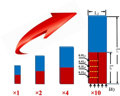
Table 2. Simulation parameters used in the validation case.

Term	Parameter	Value(s)
SCW	Pressure [MPa]	23, 25, 27
	Temperature [K]	633, 653, 693
Bed material	Type	Geldart group B
	Initial solid fraction	0.56
	ρs [kg/m^3]	2620, 2650
	ds [μm]	200, 213
Bed geometry	Domain height [m]	0.6
	Domain width [m]	0.035
	Initial bed height [m]	0.1, 0.13, 0.15, 0.2
	Grid size [m]	0.001

Note: SCW = supercritical water.

Table 3. Supercritical water (SCW) density and viscosity under different working conditions (Lu et al., 2013).

Temperature [K]	Pressure [MPa]	Density [kg/m^3]	Viscosity [Pa·s]
633	23	576.01	6.6336E-05
653	23	209.10	3.0729E-05
693	23	112.72	2.7566E-05
693	25	131.94	2.8433E-05
693	27	155.44	2.9640E-05

Figure 2 compares the effective weight of the bed materials between the current numerical results and previous experimental data (Lu et al., 2013). The predictive results, based on the equation of Yao and Lu (2017), $\mathrm{\Delta }P={\alpha }_s\left({\rho }_s-{\rho }_f\right)g{L}_0$, are also given as an additional reference. Here, the effective weight of the bed materials is equal to their actual weight after removing the buoyancy. The corresponding pressure drop value is read as an average when the superficial velocity of the SCW is beyond u_mf. It can be found in Figure 2 that the current numerical results are in line with previous results, thus showing the high accuracy of the model.

Figure 2. Comparison of the effective weight of the bed materials for the physical experiment (Lu et al., 2013), equation-predicted results (Yao & Lu, 2017) and current numerical simulation.

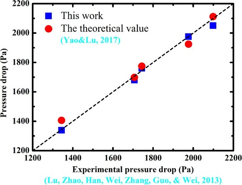
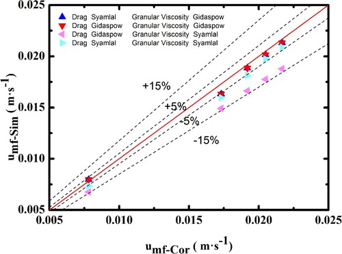
Figure 3 gives a quantitative comparison of u_mf between the experimental measurements (Lu et al., 2013) and current numerical results using different numerical models. It can be observed that the predictive errors obtained from the Gidaspow model of granular viscosity and the Syamlal model of drag force (Syamlal & O’Brien, 1989) are all below 5%, which again indicates the very good capability of these models in simulating the SCWFBR. The error here is defined as: |Experimental results − Numerical results|/Experimental results. Note that the same sets of numerical simulations are also conducted using other drag force and granular viscosity models. A comparison among these cases is helpful for selecting the optimal numerical model. All of the numerical results are provided in Figure 3, and the comparison clearly shows that the model of granular viscosity plays the dominant role in affecting the numerical accuracy. Better results can be obtained when using the Gidaspow model of granular viscosity than the Syamlal model. This is because the granular viscosity is responsible for the interlocking capability of the particle materials. A stronger interlocking capability leads to a larger minimum fluidization velocity. However, it seems that the Syamlal model of drag force performs better than the Gidaspow model. Therefore, the Gidaspow model of granular viscosity and the Syamlal model of drag force are adopted in all the numerical simulations below.

Figure 3. Comparisons of u_mf obtained by the physical experiment (Lu et al., 2013) and current numerical simulation.

A grid independence test is also conducted in this study. Here, square grids are adopted, and it is clearly seen in Table 4 that the numerical results will not be changed by further increasing the grid number. Thus, the ‘5083’ case is adopted for all calculations.

Table 4. Obtained minimum fluidization velocity based on different grid systems (P = 23 MPa, T = 633 K, d_s= 200 μm and ρ_s = 2650 kg/m³).

Cells	Minimum fluidization velocity [m/s]
1192	0.00820
5083	0.00781
20,965	0.00781

4. Results and discussion

The main aim of this section is to examine the available scale-up rule for the SCWFBR using the previously validated TFM model. Thus, four different-sized SCWFBRs are designed, as shown in Figure 1. Detailed geometric information is listed in Table 5, in which the ‘× 1’ case is used as the base case. The scale-up factors, ‘× 2’, ‘× 4’ and ‘× 10’ are exerted on the initial bed height, domain width and domain height of the base case. Therefore, the geometric similarity of these SCWFBRs can be kept during the scale-up. The working conditions are set as P = 25 MPa and T = 923 K, at which ρ_f = 64.83 kg/m³ and μ_f = 3.6415E-05 Pa·s. Note that these are the typical working conditions for the SCWFBR (Lu, Wei, et al., 2015; Yao & Lu, 2017).

Table 5. Fluidized bed reactor (FBR) geometries used in the numerical simulations.

	No.
	1	2	3	4
Scale-up factor	× 1 (base)	× 2	× 4	× 10
Domain height [m], L1	0.6	1.2	2.4	6
Domain width [m], L2	0.035	0.07	0.14	0.35
Initial bed height [m], L0	0.2	0.4	0.8	2

To make the findings of this study generalizable, two sets of numerical simulations are carried out in parallel for air–solid and SCW–solid systems. The details of these numerical simulations can be found in Tables 6 and 7, respectively. The bed material in this study can be classified as Geldart B particles. In these tables, the u_mf values for air–solid and SCW–solid systems are calculated based on the predictive correlations of Wen and Yu (1966) and Lu et al. (2013), respectively. As shown in Tables 6 and 7, a total of 16 study cases are designed, in which C01 and C09 are set as the base cases for the air–solid and SCW–solid systems, respectively. Cases C02, C03, C04, C10, C11 and C12 are scaled up according to the simplified set of scaling parameters, while the remaining cases (C06, C07, C8, C14, C15 and C16) are scaled up according to the viscous set of scaling parameters. C05 and C13 are especially designed according to the viscous set of scaling parameters but have the same size as the base cases, C01 and C09, respectively. For each study case, the numerical simulation runs for 80 s, numerical results are saved every 0.001 s and results are averaged from 20 to 80 s.

Table 6. Settings in the numerical simulations of the air–solid system.

No.	Bed	ρs [kg/m^3]	ds [μm]	u0 [m/s]	umf [m/s]	1/Fr	ρs/ρf	u0/umf	L1/L2	Res	Ar
C01	× 1	2600	300.0	0.25491	0.07587	30.19	2122	3.36	17.14	5.24	2,633
C02	× 2	2600	359.5	0.36050	0.10729	30.19	2122	3.36	17.14	8.87	4,532
C03	× 4	2600	433.2	0.50982	0.15173	30.19	2122	3.36	17.14	15.12	7,929
C04	× 10	2600	562.4	0.80610	0.23991	30.19	2122	3.36	17.14	31.04	17,350
C05	× 1	1500	396.4	0.25491	0.07586	30.19	1224	3.36	17.14	6.92	3,505
C06	× 2	3710.9	300.0	0.36050	0.10729	30.19	3029	3.36	17.14	7.40	3,759
C07	× 4	3035	400.0	0.50982	0.15173	30.19	2478	3.36	17.14	13.96	7,287
C08	× 10	3245.2	500.0	0.80610	0.23991	30.19	2649	3.36	17.14	27.59	15,219

Table 7. Settings in the numerical simulations of the supercritical water (SCW)–solid system.

No.	Bed	ρs [kg/m^3]	ds [μm]	u0 [m/s]	umf [m/s]	1/Fr	ρs/ρf	u0/umf	L1/L2	Res	Ar
C09	× 1	2650	200.0	0.06596	0.01963	451	40.88	3.36	17.14	23.48	9,918
C10	× 2	2650	247.8	0.09328	0.02776	451	40.88	3.36	17.14	41.15	18,865
C11	× 4	2650	315.5	0.13191	0.03926	451	40.88	3.36	17.14	74.09	38,943
C12	× 10	2650	467.1	0.20857	0.06208	451	40.88	3.36	17.14	173.44	126,350
C13	× 1	1500	274.0	0.06596	0.01963	451	23.14	3.36	17.14	32.17	14,158
C14	× 2	1896	300.0	0.09328	0.02776	451	29.25	3.36	17.14	49.82	23,711
C15	× 4	1797.2	400.0	0.13191	0.03926	451	27.72	3.36	17.14	93.93	53,172
C16	× 10	3344	400.0	0.20857	0.06208	451	51.58	3.36	17.14	148.52	100,647

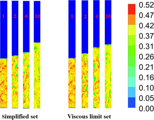
Figure 4 shows typical instantaneous distributions of the solid volume fraction in the SCW–solid system at 60 s. It can be seen that the overall flow behavior in different-sized SCWFBRs is generally similar. Owing to the difference in Re_s, the non-dimensional expansion of the bed height is observed to increase with the reactor size. To conduct a quantitative comparison in the following subsections, four heights are selected to pick the average data, as shown in the ‘× 10’ case in Figure 1, namely, 0.1L₀, 0.3L₀, 0.5L₀ and 0.9L₀. The discrepancy in numerical data at these positions will be adopted to judge the similarity among different cases.

Figure 4. Instantaneous distributions of the solid volume fraction in the supercritical water (SCW)–solid system at 60 s. Numerical results are shown using the same size as the base case for clear comparison.

4.1. Scale-up of the air–solid system

Figure 5 shows the distributions of the solid volume fraction in the air–solid system at the selected positions. It can be observed that the solid volume fraction close to the reactor boundary is lower than that near the center line. The non-uniformity of the solid volume fraction along the radial direction increases with the bed height, which is a typical phenomenon during the fluidization process. It can also be seen that both the simplified and viscous sets of scaling parameters are competent in predicting the multiphase flow behavior during the scale-up. The similarity among C01, C05 and two ‘× 2’ cases (C02 and C06) is very good in all of the selected positions. This means that both sets of scaling parameters do a very good job in scaling up the traditional gas–solid FBR of the ‘× 2’ cases. However, in both sets of scaling parameters, the degree of similarity decreases when the reactors are further scaled up to the ‘× 4’ and ‘× 10’ cases. This is mainly due to the increase in Re_s for the enlarged reactors. As seen in Figure 5, the average data for C04 are not stable owing to the high Re_s. In general, the comparison of the solid volume fraction indicates that, for the air–solid system, the viscous set of scaling parameters performs better than the simplified set, although the former was originally proposed for cases at low Re_s.

Figure 5. Distributions of the solid volume fraction in the air–solid system at selected positions: (a) h = 0.1L₀; (b) h = 0.3L₀; (c) h = 0.5L₀; (d) h = 0.9L₀.

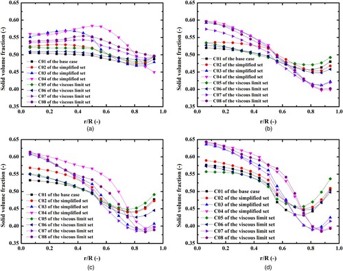
Figure 6 shows the distribution of the solid vertical velocity in the air–solid system at the selected positions, which tells almost the same story as Figure 5. The solid vertical velocity close to the boundary is low owing to the wall retardation effect. The similarity among the base case C01, C05 and the two ‘× 2’ cases is acceptable, while it becomes worse in larger reactors. From Figure 6, it is also shown that the viscous set of scaling parameters performs better than the simplified set. The superiority of the viscous set of scaling parameters over the simplified set indicates that ρ_s/ρ_f is not playing a key role in the scale-up of the air–solid system. To clearly present the capability of different scaling parameters, a relative deviation of a variable, x, is defined here as (1) $R_k\left(x\right)=\frac{\sum _{j=1}^n{\left(x_{k_j}-{\dot{x}}_{k_j}\right)}^2}{n}$(1) where k runs from 1 to 4, as mentioned earlier in Section 4, standing for different heights, 0.1L₀, 0.3L₀, 0.5L₀ and 0.9L₀, respectively, and j runs all the data acquisition points from left to right at the kth height. $\dot{x}$ is the data taken from the base cases, C01 or C09, for gas–solid or SCW–solid systems, respectively. The relative deviations for solid volume fraction and solid vertical velocity in the air–solid system are shown in Figures 7 and 8, respectively. In these figures, a short bar indicates that the relative deviation between the corresponding case and base case is small, and thus that there is a good similarity.

Figure 6. Distributions of the solid vertical velocity in the air–solid system at selected positions: (a) h = 0.1L₀; (b) h = 0.3L₀; (c) h = 0.5L₀; (d) h = 0.9L₀.

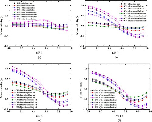
Figure 7. Relative deviations for solid volume fraction in the air–solid system between different cases with C01. Details are given in Figure 5.

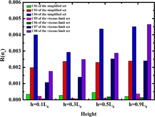
Figure 8. Relative deviations for solid vertical velocity in the air–solid system between different cases with C01. Details are given in Figure 6.

The results in Figures 7 and 8 are exactly the same as those in Figures 5 and 6, but are shown in a much clearer way. By carefully examining Table 6, it is found that, in addition to the considered scaling parameters, d_s, Re_s and Ar may have a great influence on the scaled numerical results; these are expressed as (2) $\begin{array}{rl}Ar& =\frac{d_s^2{\rho }_f({\rho }_s-{\rho }_f)g}{{\mu }_s^2}\end{array}$(2) (3) $\begin{array}{rl}R{e}_{mf}& =(C_1^2+C_{2}Ar{)}^{0.5}-C_1\end{array}$(3) where C₁ and C₂ are constants. In other words, keeping any or all of these three parameters constant may lead to better similarity during the scale-up. Since Re_mf ∝ Re_s in this study, the roles of Re_s and Ar are equivalent and thus only Re_s is considered below. The discussion on the roles of Re_s and d_s is continued by checking more numerical results. Before this, the overall performance of the two sets of scaling parameters for the air–solid system is shown in Figure 9, which is based on the data of the solid volume fraction. The exact value of |C0i–C01| here does not make physical sense but is only an indicator to show the similarity of different cases with C01. Lower |C0i–C01| stands for higher similarity. A global comparison indicates that the similarity decreases from C06, C02, C05, C07, C03, C08 to C04, and decreases with the increase in the difference of their d_s. It can be clearly seen that the viscous set of scaling parameters performs better than the simplified set for each equally sized reactor (|C06–C01| < |C02–C01|, |C07–C01| < |C03–C01| and |C08–C01| < |C04–C01|).

Figure 9. Overall performance of two sets of scaling parameters for the air–solid system.

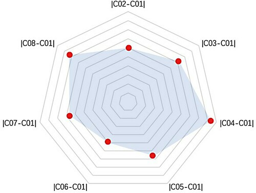
Furthermore, it can be observed that the similarity between C01 and C06 is the closest when they have the same particle diameter, d_s. This finding leads the authors to conclude that both Re_s and d_s are critical for maintaining the similarity during the scale-up of the air–solid system. Re_s plays the dominant role in keeping the multiphase flow behavior similar, which is consistent with the full set of scaling parameters (Glicksman, 1984). Contrary to the full set (Glicksman, 1984), the current numerical results indicate that the more similar d_s is, the more similar the multiphase flow behavior will be. In other words, to maintain the similarity, it is practical to keep Re_s constant during the scale-up. To do so, one should keep d_s fixed while tuning other variables to reach the same Re_s. The particle diameter, d_s, should not be enlarged with the reactor size following a constant L₀/d_s, as required by the full set of scaling parameters (Glicksman, 1984).

4.2. Scale-up of the SCW–solid system

Figure 10 shows the relative deviations of the solid volume fraction in the SCW–solid system at the selected positions. Similarly to the air–solid system, Figure 10 shows that both sets of scaling parameters can do a very good job in scaling up the SCWFBR of the ‘× 2’ cases. In contrast to the gas–solid system, it is found that the simplified set of scaling parameters performs better than the viscous set for the SCWFBR, indicating that ρ_s/ρ_f plays a critical role in the scale-up of the SCWFBR. This is mainly because the ρ_f of SCW is much larger than that of gas, which is comparable with ρ_s. When comparing the base case C09 and the scaled cases, it is not difficult to find that keeping Re_s similar can lead to a good similarity of the solid volume fraction, even though they may have quite different values of d_s or ρ_s/ρ_f. The high correlation between the similarity and Re_s is also in line with that for the air–solid system and the full set of scaling parameters (Glicksman, 1984).

Figure 10. Relative deviations for solid volume fraction in the supercritical water (SCW)–solid system between different cases with C09.

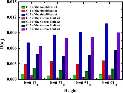
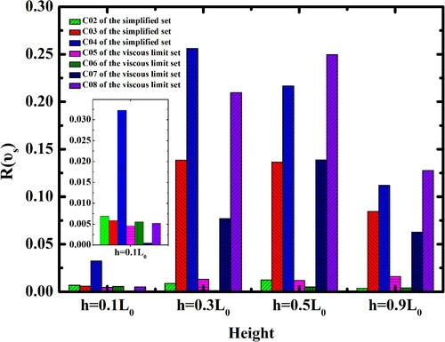
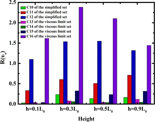
Figure 11 shows the relative deviations of the solid vertical velocity in the SCW–solid system at the selected positions. In general, it can be seen that the influence of Re_s on the similarity of the compared cases is obvious. That is, when the difference in Re_s between the two cases is large, the similarity becomes poor. However, combining Table 7 and Figure 11, one can find that the similarity of the solid vertical velocity among the cases does not strictly follow the difference in Re_s. This may be due to the large density of SCW causing large drag forces on the solid particles and strongly affecting their motion. As a result, the influence of the interparticle collisions increases with Re_s and thus introduces more fluctuation to the solid vertical velocity at high Re_s. Therefore, the effect of interparticle collisions should be considered in the scaling parameters for the SCW–solid system (Jong & Ommen, 2009; Maio & Renzo, 2013).

Figure 11. Relative deviations for solid vertical velocity in the supercritical water (SCW)–solid system between different cases with C09.

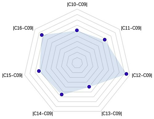
The relative deviations of pressure in the SCW–solid system at the selected positions are further examined in Figure 12. It can be observed that the changing trend in pressure with Re_s has perfect agreement with the solid volume fraction. Therefore, the overall performance of two sets of scaling parameters for the SCW–solid system can be presented as Figure 13, in which the similarity between the base and scaled cases increases with the decrease in the difference of their Re_s. The overall performance of the two sets of scaling parameters for the SCW–solid system is shown in Figure 13. It can be seen that the viscous set of scaling parameters performs better than the simplified set for each equally sized reactor (|C10–C09| < |C14–C09|, |C11–C09| < |C15–C09|, but |C12–C01| > |C16–C09|).

Figure 12. Relative deviations for pressure in the supercritical water (SCW)–solid system between different cases with C09.

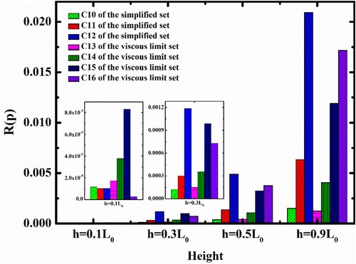
Figure 13. Overall performance of two sets of scaling parameters for the supercritical water (SCW)–solid system.

5. Concluding remarks

In this paper, numerical simulations are carried out based on the TFM. The numerical results are used to examine the capability of different scale-up rules for the SCWFBR. Four different-sized SCWFBRs are designed and the distributions of solid volume fraction, solid velocity and pressure in these reactors are investigated. From a critical comparison, the following conclusions can be drawn:

1. The parameters < Re_s, Fr = (u₀)²/(gL₀), u₀/u_mf, L₁/L₂ and Φ > can be used to guide the scale-up of the traditional gas–solid FBR, although the similarity can drop with the increase in the reactor size. Furthermore, to keep Re_s constant during the scale-up, it is ideal to keep d_s constant while tuning other relevant parameters.

2. For the SCW–solid system, < Re_s, Fr = (u₀)²/(gL₀), ρ_s/ρ_f, u₀/u_mf, L₁/L₂ and Φ > can be used to guide the scale-up. The additional limit of ρ_s/ρ_f on the traditional gas–solid FBR is a result of the large SCW density, which also leads to more active particle motions. Finally, the effect of interparticle collisions should be considered in the scaling parameters for the SCW–solid system at high Re_s.

It must be mentioned that the current work only contains cold models describing flow patterns. Therefore, a more detailed study via hot (Ye et al., 2020) and complex models (Zhang et al., 2021) on the temperature and species distributions in different-sized reactors could provide more accurate guidelines for scale-up in future work. Furthermore, the combination of machine learning and computational fluid dynamics (CFD) data (Ghazvinei et al., 2018; Mosavi et al., 2019; Shamshirband et al., 2020) has been drawing tremendous attention in efforts to predict the macroscopic and microscopic hydrodynamic parameters of various FBRs. Such successful combinations will lead to a further reduction in computational cost during the design when considering big data. In this way, a true three-dimensional simulation of an actual industrial-scale reactor could be made available. It must be admitted that the information provided by two-dimensional numerical results is quite limited; however, a two-dimensional simulation may be enough, as a first and cheaper approach, to capture the general features of the multiphase flow pattern. Three-dimensional simulations are necessary for an accurate description of the flow.

Nomenclature

$Ar$	=	Number of geometric properties [–]
$CD$	=	Drag coefficient [–]
$d_s$	=	Particle diameter [m]
$e_{ss}$	=	Coefficient of restitution for particle collisions [–]
$Fr$	=	Froude number [–]
$f$	=	Fluid phase (subscript)
$\overrightarrow{g}$	=	Gravity acceleration [m/s2]
$g_{o,ss}$	=	Radial distribution function [–]
$h$	=	Bed height [m]
$\overline{\overline{I}}$	=	Unit tensor [Pa]
$I_{2D}$	=	Second invariant of the deviatoric stress tensor [Pa]
$K_{fs}$	=	Interphase drag coefficient [–]
$k_{{\mathrm{\Theta }}_s}$	=	Diffusion coefficient [–]
$L_0$	=	Initial bed height [m]
$L_1$	=	Domain height [m]
$L_2$	=	Domain width [m]
$p$	=	Pressure by all phases [Pa]
$p_{friction}$	=	Frictional pressure [Pa]
$p_s$	=	Solid pressure [Pa]
$R{e}_{mf}$	=	Reynolds number based on minimum fluidization velocity [–]
$R{e}_s$	=	Reynolds number [–]
$s$	=	Solid phase (subscript)
$u_0$	=	Velocity of fluid [m/s]
$u_{mf}$	=	Minimum fluidization velocity [m/s]
$\overrightarrow{v}$	=	Velocity [m/s]
${\nu }_{r,s}$	=	Terminal velocity correlation for the solid phase [m/s]
$\alpha$	=	Volume fraction [–]
${\alpha }_{s,max}$	=	Packing limit [–]
${\mathrm{\Theta }}_s$	=	Granular temperature [K]
$\lambda$	=	Bulk viscosity [kg/(m·s)]
$\mu$	=	Shear viscosity [kg/(m·s)]
${\mu }_{s,col}$	=	Solid collision viscosity [kg/(m·s)]
${\mu }_{s,fr}$	=	Solid frictional viscosity [kg/(m·s)]
${\mu }_{s,kin}$	=	Solid kinetic viscosity [kg/(m·s)]
$\rho$	=	Density [kg/m3]
${\overline{\overline{\tau }}}_f$	=	Fluid phase stress–strain tensor [Pa]
${\overline{\overline{\tau }}}_s$	=	Solid phase stress–strain tensor [Pa]
${\gamma }_{{\mathrm{\Theta }}_s}$	=	Collisional dissipation of energy [–]
$\mathrm{\Phi }$	=	Degree of sphericity
$\phi$	=	Angle of internal friction [°]
${\phi }_{fs}$	=	Energy exchange between the fluid phase and solid phase [–]

Acknowledgments

The authors sincerely acknowledge the National Natural Science Foundation of China and the Natural Science Foundation of Liaoning Province for the financial support on this research.

Disclosure statement

No potential conflict of interest was reported by the authors.

Additional information

Funding

This work was supported by National Natural Science Foundation of China [grant number 12072071]; Natural Science Foundation of Liaoning province [grant number 2019-MS-125]; National Key R&D Program of China [grant number 2016YFB0600101-4].

References

- Bashiri, H., Mostoufi, N., Radmanesh, R., Sotudehgharebagh, R., & Chaouki, J. (2010). Effect of bed diameter on the hydrodynamics of gas-solid fluidized beds. Iranian Journal of Chemistry and Chemical Engineering, 29(3), 27–36. https://doi.org/http://doi.org/10.1016/j.ijrmhm.2010.06.003
- Boemer, A., Qi, H., & Renz, U. (1998). Verification of Eulerian simulation of spontaneous bubble formation in a fluidized bed. Chemical Engineering Science, 53(10), 1835–1846. https://doi.org/https://doi.org/10.1016/S0009-2509(98)00044-X
- Bonniol, F., Sierra, C., Occelli, R., & Tadrist, L. (2009). Similarity in dense gas–solid fluidized bed, influence of the distributor and the air-plenum. Powder Technology, 189(1), 14–24. https://doi.org/https://doi.org/10.1016/j.powtec.2008.05.011
- Bricout, V., & Louge, M. Y. (2004). A verification of Glicksman’s reduced scaling under conditions analogous to pressurized circulating fluidization. Chemical Engineering Science, 59(13), 2633–2638. https://doi.org/https://doi.org/10.1016/j.ces.2004.03.017
- Correa, C. R., & Kruse, A. (2017). Supercritical water gasification of biomass for hydrogen production – Review. The Journal of Supercritical Fluids, 133, 573–590. https://doi.org/https://doi.org/10.1016/j.supflu.2017.09.019
- Ebrahimi, M., Siegmann, E., Prieling, D., Glasser, B. J., & Khinast, J. G. (2017). An investigation of the hydrodynamic similarity of single-spout fluidized beds using CFD-DEM simulations. Advanced Powder Technology, 28(10), 2465–2481. https://doi.org/https://doi.org/10.1016/j.apt.2017.05.009
- Ghazvinei, P. T., Darvishi, H. H., Mosavi, A., Yusof, K., Alizamir, M., & Shamshirband, S. (2018). Sugarcane growth prediction based on meteorological parameters using extreme learning machine and artificial neural network. Engineering Applications of Computational Fluid Mechanics, 12(1), 738–749. https://doi.org/https://doi.org/10.1080/19942060.2018.1526119
- Glicksman, L. R. (1984). Scaling relationships for fluidized beds. Chemical Engineering Science, 39(9), 1373–1379. https://doi.org/https://doi.org/10.1016/0009-2509(84)80070-6
- Glicksman, L. R. (1988). Scaling relationships for fluidized beds. Chemical Engineering Science, 43(6), 1419–1421. https://doi.org/https://doi.org/10.1016/0009-2509(88)85118-2
- Glicksman, L. R., Hyre, M., & Woloshun, K. (1993). Simplified scaling relationships for fluidized beds. Powder Technology, 77(2), 177–199. https://doi.org/https://doi.org/10.1016/0032-5910(93)80055-F
- Glicksman, L. R., Hyre, M. R., & Farrell, P. A. (1994). Dynamic similarity in fluidization. International Journal of Multiphase Flow, 20, 331–386. https://doi.org/https://doi.org/10.1016/0301-9322(94)90077-9
- Horio, M., Nonaka, A., Sawa, Y., & Muchi, I. (1986). A new similarity rule for fluidized bed scale-up. AICHE Journal, 32(9), 1466–1482. https://doi.org/https://doi.org/10.1002/aic.690320908
- Jong, W. D., & Ommen, J. R. V. 2019. Scale-up in fluidized bed biomass combustion, 33–60.
- Kelkar, V. V., & Ng, K. M. (2002). Development of fluidized catalytic reactors: Screening and scale-up. AICHE Journal, 48(7), 1498–1518. https://doi.org/https://doi.org/10.1002/aic.690480714
- Knowlton, T. M., Karri, S., & Issangya, A. (2005). Scale-up of fluidized-bed hydrodynamics. Powder Technology, 150(2), 72–77. https://doi.org/https://doi.org/10.1016/j.powtec.2004.11.036
- Lu, B., Zhang, J., Luo, H., Wang, W., Li, H., & Ye, M. (2017). Numerical simulation of scale-up effects of methanol-to-olefins fluidized bed reactors. Chemical Engineering Science, 171, 244–255. https://doi.org/https://doi.org/10.1016/j.ces.2017.05.007
- Lu, Y., Huang, J., Zheng, P., & Jing, D. (2015). Flow structure and bubble dynamics in supercritical water fluidized bed and gas fluidized bed: A comparative study. International Journal of Multiphase Flow, 73, 130–141. https://doi.org/https://doi.org/10.1016/j.ijmultiphaseflow.2015.03.011
- Lu, Y., Wei, L., & Wei, J. (2015). A numerical study of bed expansion in supercritical water fluidized bed with a non-spherical particle drag model. Chemical Engineering Research & Design, 104, 164–173. https://doi.org/https://doi.org/10.1016/j.cherd.2015.08.005
- Lu, Y., Zhang, T., & Dong, X. (2016). Numerical analysis of heat transfer and solid volume fraction profiles around a horizontal tube immersed in a supercritical water fluidized bed. Applied Thermal Engineering, 93, 200–213. https://doi.org/https://doi.org/10.1016/j.applthermaleng.2015.09.026
- Lu, Y., Zhao, L., & Guo, L. (2011). Technical and economic evaluation of solar hydrogen production by supercritical water gasification of biomass in China. International Journal of Hydrogen Energy, 36(22), 14349–14359. https://doi.org/https://doi.org/10.1016/j.ijhydene.2011.07.138
- Lu, Y., Zhao, L., Han, Q., Wei, L., Zhang, X., & Guo, L. (2013). Minimum fluidization velocities for supercritical water fluidized bed within the range of 633-693K and 23-27MPa. International Journal of Multiphase Flow, 49, 78–82. https://doi.org/https://doi.org/10.1016/j.ijmultiphaseflow.2012.10.005
- Maio, F., & Renzo, A. D. (2013). Verification of scaling criteria for bubbling fluidized beds by DEM–CFD simulation. Powder Technology, 248, 161–171. https://doi.org/https://doi.org/10.1016/j.powtec.2013.03.029
- Matsen, J. M. (1996). Scale-up of fluidized bed processes: Principle and practice. Powder Technology, 88(3), 237–244. https://doi.org/https://doi.org/10.1016/S0032-5910(96)03126-9
- Matsen, J. M. (1997). Design and scale-up of CFB catalytic reactors. Springer Netherlands.
- Matsumura, Y., & Minowa, T. (2004). Fundamental design of a continuous biomass gasification process using a supercritical water fluidized bed. International Journal of Hydrogen Energy, 29(7), 701–707. https://doi.org/https://doi.org/10.1016/j.ijhydene.2003.09.005
- Mosavi, A., Shamshirband, S., Salwana, E., Chau, K. W., & Tah, J. (2019). Prediction of multi-inputs bubble column reactor using a novel hybrid model of computational fluid dynamics and machine learning. Engineering Applications of Computational Fluid Mechanics, 13(1), 482–492. https://doi.org/https://doi.org/10.1080/19942060.2019.1613448
- Okolie, J. A., Rana, R., Nanda, S., Dalai, A. K., & Kozinski, J. A. (2019). Supercritical water gasification of biomass: A state-of-the-art review of process parameters, reaction mechanisms and catalysis. Sustainable Energy & Fuels, 3(3), 578–598. https://doi.org/https://doi.org/10.1039/C8SE00565F
- Ommen, J., Teuling, M., Nijenhuis, J., & Wachem, B. (2006). Computational validation of the scaling rules for fluidized beds. Powder Technology, 163(1-2), 32–40. https://doi.org/https://doi.org/10.1016/j.powtec.2006.01.010
- Ren, C., Jin, H., Ren, Z., Ou, Z., & Guo, L. (2020). Simulation of solid-fluid interaction in a supercritical water fluidized bed with a cold jet. Powder Technology, 363, 687–698. https://doi.org/https://doi.org/10.1016/j.powtec.2020.01.034
- Rüdisüli, M., Schildhauer, T. J., Biollaz, S. M. A., & van Ommen, J. R. (2012). Scale-up of bubbling fluidized bed reactors – A review. Powder Technology, 217, 21–38. https://doi.org/https://doi.org/10.1016/j.powtec.2011.10.004
- Shamshirband, S., Babanezhad, M., Mosavi, A., Nabipour, N., Hajnal, E., & Nadai, L. (2020). Prediction of flow characteristics in the bubble column reactor by the artificial pheromone-based communication of biological ants. Engineering Applications of Computational Fluid Mechanics, 14(1), 367–378. https://doi.org/https://doi.org/10.1080/19942060.2020.1715842
- Syamlal, M., & O’Brien, T. J. (1989). Computer simulation of bubbles in a fluidized bed. AICHE Symposium Series, 8, 22–31.
- Verma, V., Padding, J. T., Deen, N. G., & Kuipers, J. (2015). Effect of bed size on hydrodynamics in 3-D gas–solid fluidized beds. AICHE Journal, 61(5), 1492–1506. https://doi.org/https://doi.org/10.1002/aic.14738
- Wagner, W., Cooper, J. R., Dittmann, A., Kijima, J., Kretzschmar, H., Kruse, A., Mares, R., Oguchi, K., Sato, H., & Stocker, I. (2000). The IAPWS industrial formulation 1997 for the thermodynamic properties of water and steam. Journal of Engineering for Gas Turbines & Power, 122(1), 150–184. https://doi.org/https://doi.org/10.1115/1.483186
- Wang, Q., Zhang, K., Brandani, S., & Jiang, J. (2009). Scale-up strategy for the jetting fluidized bed using a CFD model based on two-fluid theory. The Canadian Journal of Chemical Engineering, 87(2), 204–210. https://doi.org/https://doi.org/10.1002/cjce.20148
- Wei, L., Lu, Y., & Wei, J. (2013). Hydrogen production by supercritical water gasification of biomass: Particle and residence time distribution in fluidized bed reactor. International Journal of Hydrogen Energy, 38(29), 13117–13124. https://doi.org/https://doi.org/10.1016/j.ijhydene.2013.01.148
- Wen, C. Y., & Yu, Y. H. (1966). A generalized method for predicting the minimum fluidization velocity. AICHE Journal, 12(3), 610–612. https://doi.org/https://doi.org/10.1002/aic.690120343
- Werther, J. (1974). Influence of the bed diameter on the hydrodynamics of gas fluidized beds. ACS Symposium Series, 70(141), 53–62.
- Wu, G., Wang, Q., Zhang, K., & Wu, X. (2016). CFD simulation of hydrodynamics and heat transfer for scale-up of the jetting fluidized beds. Powder Technology, 304, 120–133. https://doi.org/https://doi.org/10.1016/j.powtec.2016.08.021
- Yao, L., & Lu, Y. (2017). Supercritical water gasification of glucose in fluidized bed reactor: A numerical study. International Journal of Hydrogen Energy, 42(12), 7857–7865. https://doi.org/https://doi.org/10.1016/j.ijhydene.2017.03.009
- Ye, X., An, X., Zhang, H., & Guo, B. (2020). Numerical simulation on flow and evaporation characteristics of desulfurization wastewater in a bypass flue. Engineering Applications of Computational Fluid Mechanics, 14(1), 411–421. https://doi.org/https://doi.org/10.1080/19942060.2020.1719891
- Zhang, H., Huang, Y., An, X., Yu, A., & Xie, J. (2021). Numerical prediction on the minimum fluidization velocity of in a supercritical water fluidized bed reactor: Effect of particle size distributions. Powder Technology, 389, 119–130. https://doi.org/https://doi.org/10.1016/j.powtec.2021.05.015
- Zhong, W., Liu, X., Grace, J. R., Epstein, N., Ren, B., & Jin, B. (2013). Prediction of minimum spouting velocity of spouted bed by CFD-TFM: Scale-up. Canadian Journal of Chemical Engineering, 91(11), 1809–1814. https://doi.org/https://doi.org/10.1002/cjce.21865