Evaluating shallow mixing layer in partially-distributed canopy flows using DA-LES: bed friction, water shallowness and canopy denseness

ABSTRACT

Shallow mixing layers developed in partially-distributed canopy flows (PCFs) are important for water conveyance, sediment transport and solute dispersion. In this paper, we address the response of shallow mixing layers in PCFs to several influential factors associated with bed friction, water shallowness and canopy denseness using depth-averaged Large Eddy Simulation (DA-LES). The results show that under certain canopy denseness, shallow mixing layers in PCFs display asymptotic behaviour for the variation of bed friction and water shallowness, consistent with classic shallow mixing layers. The canopy drag encourages the asymmetric growth of the inner and outer parts of the mixing layer, and this effect decreases when bed friction and water shallowness become pronounced. Characteristic velocity and length scales show similarity well delineated by exponential decay function regarding a stabilization efficiency parameter. The exception happens for the inner length scale of the mixing layer when only changing canopy density. We conclude that changing the canopy denseness can encourage the overall shift of mixing layer scaling regarding a broad range of bed friction and water shallowness. Furthermore, the bed friction parameter thresholding triggering flow instability of mixing layers in PCFs is found about 0.03, lower than 0.09 for splitter-plate induced mixing layers.

KEYWORDS:

• Shallow mixing layers
• partially-distributed canopy flows
• characteristic scales
• stabilization efficiency
• scaling shift

1. Introduction

Riparian/near-bank vegetation is commonly observed to extend longitudinally, forming porous obstructive canopies partially across open surface waters such as rivers, streams and wetlands (Guo et al., 2020; Gurnell et al., 2001). The continuity in vegetative drag alters transversely, leading to a significant lateral shear interface (Yan et al., 2022a), triggering horizontal flow instability (de Lima & Izumi, 2014), and inducing lateral spatial distribution in flow velocity and bed shear stress (Nezu & Onitsuka, 2001). Consequently, flow conveyance, sediment transport and solute dispersion are re-adjusted compared with non-vegetated water courses. It has been shown that the transformation of hydrodynamics has sound impacts on fluvial processes (Gurnell, 2014; Xu et al., 2020), environment conservation (Chen & Cho, 2019; Li et al., 2023) and flood routes (Anderson et al., 2006; van Zelst et al., 2021).

Lateral canopy shears are fundamental hydrodynamic features in partially-distributed canopy flows (PCFs), which have been broadly addressed by previous studies. White and Nepf (2007) observed that a lateral shear layer grew in the adjacent outer zone, and velocity profiles for different scenarios can collapse onto a general curve with proper characteristic scales (velocity scale and length scale). On the other hand, horizontal flow instability is the cause of canopy-scale vortices, causing high momentum of the outer zone penetrating into the neighbouring canopy interior and producing mixing-layer-type lateral profiles of longitudinal velocity (Figure 1). The penetration distance was found associated with the resistance capability of the canopy, which was linked with a canopy drag scale (C_da)⁻¹ (Nepf, 2012; White & Nepf, 2008). With the momentum balance equation averaged over water depth and these scaling scales, the solution of depth-averaged velocity at equilibrium can be achieved for different canopy and flow configurations (Ben Meftah et al., 2014; Liu & Shan, 2019; Meftah & Mossa, 2016; White & Nepf, 2008).

Figure 1. Conceptual sketch of partially-distributed canopy flows (PCFs).

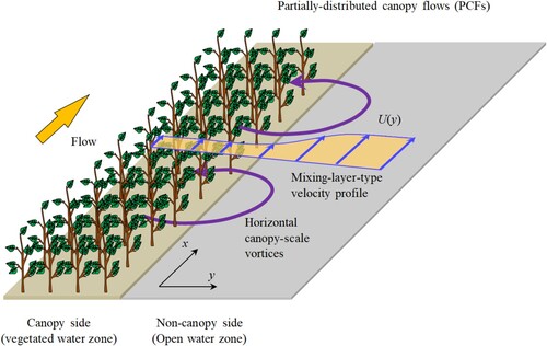
Horizontal canopy-scale vortices are important to adjust the lateral-distributed flow structure by altering lateral mixing and thus turbulence viscosity (Ben Meftah et al., 2014; White & Nepf, 2007, 2008; Zhang et al., 2023). Due to the occurrence of lateral velocity shear, PCFs can be comparable to typical shallow mixing layers such as splitter plate flows and compound channel flows (Chu & Babarutsi, 1988; Ghidaoui & Kolyshkin, 1999). For this type of flow referred to as shallow mixing layers, understanding the effects of bed friction and water shallowness is important for completing the generalization of shallow mixing layers and horizontal coherent vortices in PCFs. For a shallow mixing layer, the mixing layer width is likely to be suppressed by a rougher bottom and shallower water due to the stabilization effect. A bed friction parameter incorporating the effects of bed friction and water shallowness can be used to evaluate the stability of the shallow mixing layer. A judgement criterion is that for this parameter <0.09 horizontal flow instability can be generated for splitter-plate-induced shallow mixing layers (Chu & Babarutsi, 1988). For PCFs, Nepf (2012) also noted that the scenario of ah > 0.1 (a is the canopy density and h is the flow depth) triggered canopy-scale vortices. The effects of bed friction and water shallowness, however, were assumed negligible.

The effects of bed friction and water shallowness on lateral mixing layers in PCFs have not been systematically examined with experimentation and numerical modelling. However, several linear and nonlinear stability analysis works have been carried out for the examination of these effects (de Lima & Izumi, 2014; Lima & Izumi, 2011). According to the theoretical results, the interface oscillating flow motions are likely to be stabilized in the range of high bed shear effect, moderate Froude number and sufficiently small and large vegetation densities. The former two effects essentially accounting for bed friction and water shallowness for PCFs are consistent with common shallow mixing layers. However, these studies cannot provide insights into the response and quantification of characteristic scales of shallow mixing layers in PCFs to associated influential factors, which thus motivates this study.

Modelling the hydrodynamics of canopy flows has been implemented for decades. For s partially-distributed setting, both Reynolds-averaged and large-eddy numerical methods have been reported for the modelling. For three-dimensional modelling, Su and Li (2002) conducted a LES modelling of PCFs, and showed the formation of the KH vortices. Yan et al. (2016) improved the Spalart-Allmrous turbulence model with the physically accurate representation of the characteristic length scale and successfully reproduced the near-bed velocity deflection in the junction region of submerged-type PCFs. The above two studies formulated the canopy drag as a sink term in the governing equations and focused on the large-scale vortex dynamics on the flow fields, which saved the computational cost. Mapping the grids on the entire solid boundaries (including vegetation stems), Huai et al. (2015), Liu et al. (2022) and Koken and Constantinescu (2023) visualize the both canopy-scale vortices and stem-scale wakes for PCFs and the three-dimensional effects of vortex evolution. Since the full-dimensional modelling of PCFs even for Reynolds-averaged methods is computationally costly, the above studies focused on a few modelling scenarios and examined the mechanical matters.

Owing to shallow water problem that the horizontal dimension of the flow motion substantially prevails over the vertical dimension, depth-averaged modelling is prevalent in modelling water and sediment movement problems (Duan & Nanda, 2006; Hinterberger et al., 2007; Lazzarin & Viero, 2023; Molls & Chaudhry, 1995; Wu, 2004; Xu et al., 2020; Yan et al., 2022b; Yang et al., 2013). Intuition and applied mathematics suggest that three-dimensional numerical modelling should be more accurate than the depth-averaged version since the flow of full dimensions is resolved. However, due to complex boundaries and computational grids, depth-averaged modelling might be more appropriate for some particular cases. For example, Lloyd and Stansby (1997) compared the depth-averaged modelling and three-dimensional modelling of flow around a conical island which is a typical shallow water problem, and the results showed that the depth-averaged modelling prevailed over the 3D modelling. Kasvi et al. (2015) argued that the modelling performances of 2D and 3D hydro-morphological models for a real meander were quite equivalent. For PCFs, the mean and fluctuating flow motions are horizontal due to the production of horizontal canopy-scale vortices. Compared with the flow around an obstacle, PCFs should be more subjected to shallow waters, since no significant large-scale vortices such as horseshoe vortex structure that is three-dimensional are likely to be generated. Depth-averaged Large Eddy Simulation (DA-LES) was reported to effectively capture the time-mean depth-averaged flow fields and periodically-oscillating instantaneous flow field in PCFs (Jia et al., 2022; Nadaoka & Yagi, 1998), with the bottom-induced turbulence represented by a subdepth scale turbulence model (Elder, 1959). These arguments justify the applicability of the DA-LES approach in evaluating the hydrodynamic behaviour of shallow mixing layers in PCFs influenced by various impacts, particularly concentrating on canopy-scale vortices only. More importantly, with a lower computational burden, the DA-LES can encourage a statistical analysis of shallow mixing layers in PCFs in analogy to previous studies of other shallow mixing layers.

In this paper, we aim to address the effects of bed friction and water shallowness in stabilizing the horizontal oscillating flow motion and thus suppressing shallow mixing layers in PCFs. The effect of canopy denseness is also examined. A well-validated DA-LES model (Jia et al., 2022) is used to produce a fundamental depth-averaged instantaneous flow velocity field for analyzing time-mean velocity, Reynolds shear stress and characteristic scales of shallow mixing layers in PCFs. Particular attention is placed on whether the similarity of shallow mixing layers in PCFs exists across a broad range of bed friction, water shallowness and canopy denseness.

2. Methodology

The assessment of vortex evolution and associated depth-averaged hydrodynamics needs to resolve at least the horizontal large-scale vortices with the governing equations and model the subdepth scale turbulence rising from the bottom. This can be done with the implementation of depth-averaged LES (DA-LES) modelling embedded in Nays2DH.

2.1. Mathematical model

To solve large-scale motions of shallow waters, a spatial filter is applied to remove small-scale motions that are not resolvable due to grid size restriction. The corresponding governing equations are as follows.

Continuity equation. (1) $\begin{array}{r}\frac{\mathrm{\partial }h}{\mathrm{\partial }t}+\frac{\mathrm{\partial }\left(\mathrm{hu}\right)}{\mathrm{\partial }x}+\frac{\mathrm{\partial }\left(\mathrm{hv}\right)}{\mathrm{\partial }y}=0\end{array}$(1)

Momentum equations (2) $\begin{array}{rl}& \frac{\mathrm{\partial }\left(\mathrm{hu}\right)}{\mathrm{\partial }t}+\frac{\mathrm{\partial }\left(h{u}^2\right)}{\mathrm{\partial }x}+\frac{\mathrm{\partial }\left(\mathrm{huv}\right)}{\mathrm{\partial }y}=-\mathrm{gh}\frac{\mathrm{\partial }\eta }{\mathrm{\partial }x}+T_x-\frac{{\tau }_{\mathrm{bx}}}{\rho }+\frac{F_x}{\rho }\end{array}$(2) (3) $\begin{array}{rl}& \frac{\mathrm{\partial }\left(\mathrm{hv}\right)}{\mathrm{\partial }t}+\frac{\mathrm{\partial }\left(\mathrm{huv}\right)}{\mathrm{\partial }x}+\frac{\mathrm{\partial }\left(h{v}^2\right)}{\mathrm{\partial }y}=-\mathrm{gh}\frac{\mathrm{\partial }\eta }{\mathrm{\partial }y}+T_y-\frac{{\tau }_{\mathrm{by}}}{\rho }+\frac{F_y}{\rho }\end{array}$(3) (4) $\begin{array}{rl}& {\tau }_{\mathrm{bx}}=\rho C_{f}u\sqrt{u^2+v^2},{\tau }_{\mathrm{by}}=\rho C_{f}v\sqrt{u^2+v^2}\end{array}$(4) (5) $\begin{array}{rl}& F_x=\frac{1}{2}\rho C_d\mathrm{ahu}\sqrt{u^2+v^2},F_y=\frac{1}{2}\rho C_d\mathrm{ahv}\sqrt{u^2+v^2}\end{array}$(5) where t is the time, x and y are longitudinal and transverse coordinates, u and v are longitudinal and transverse velocity components, h is the water depth, η is the surface level, ρ is the fluid density, T_x and T_y are longitudinal and transverse components of stresses acting on the water body, τ_bx and τ_by are the longitudinal and transverse components of bed shear stress, F_x and F_y are longitudinal and transverse components of vegetative drag force, C_d is the drag coefficient, a is the canopy density, and c_f is the bed friction coefficient determined by Manning's roughness coefficient n_m with $c_f=g{n}_m^2/h^{1/3}$.

The variables (u, v and h) to be solved represent spatially averaged ones. Generally, the grid size for capturing large-scale motions should be sufficiently fine. Therefore, the spatial averaging (filtering) of the original Navier-Stokes equations leaves extra stress terms (T_x and T_y), imposing dispersive effects on the resolved flow. For a depth-averaged problem, the stress terms should incorporate the effect of both unsolved horizontal motions and subdepth scale turbulence. Basically, the grid size is fine enough for the 2D motions, particularly for horizontally large-scale-vortex-dominated shallow waters. Only the subdepth scale turbulence needs to be modelled (Hinterberger et al., 2007; Nadaoka & Yagi, 1998). The subdepth scale turbulence arises from the interaction between flow and bottom vertically, and this effect theoretically adds a 3D turbulence effect in the depth-averaged modelling. Previous modelling works regarding DA-LES or 2D unsteady Reynolds-averaged Navier-Stokes (URANS) employed a simple formulation that correlates the eddy viscosity (v_t) from the subdepth scale turbulence to the local hydrodynamics, (6) $\begin{array}{r}{\nu }_t=\frac{\kappa }{6}h{u}_{\ast }\end{array}$(6) where u_* is the eddy viscosity and κ is the von Kármán constant equal to 0.4.

Through the relationship between stresses, strain rate and eddy viscosity, (7) $\begin{array}{rl}{T}_x& =\frac{\mathrm{\partial }}{\mathrm{\partial }x}\left({\nu }_{t}h\frac{\mathrm{\partial }u}{\mathrm{\partial }x}\right)+\frac{\mathrm{\partial }}{\mathrm{\partial }y}\left({\nu }_{t}h\frac{\mathrm{\partial }u}{\mathrm{\partial }y}\right),\\ T_y& =\frac{\mathrm{\partial }}{\mathrm{\partial }x}\left({\nu }_{t}h\frac{\mathrm{\partial }v}{\mathrm{\partial }x}\right)+\frac{\mathrm{\partial }}{\mathrm{\partial }y}\left({\nu }_{t}h\frac{\mathrm{\partial }v}{\mathrm{\partial }y}\right)\end{array}$(7)

The governing equations can be finally closed.

It is worth noting that mathematically the stress terms play roles in diffusing variable gradients or enhancing the mixing process. Pronounced stresses may tend to stabilize flow and depress large-scale vortices. Operationally, a factor is thus used to multiply Equation (6) and a sensitive study is conducted, finding the appropriate factor = 0.2.

The finite difference method is applied to discretize the governing equations on a structured mesh. The cubic interpolated pseudoparticle (CIP) method is used as the numerical scheme with a third order to obtain the numerical solution in an explicit form. The numerical method solves boundary problems while introducing little numerical diffusion, and algorithm implementation is more straightforward than for other high-order upwind (Jang & Shimizu, 2005, 2007). The aim of this study is to assess the behaviour of the vortex during evolution impacted by the variable canopy blocking ratio rather than the spatial distribution after flow entering the canopy reach. Therefore, periodic boundary conditions are applied with a low cost grid system and computational domain. However, the computational domain (longitudinal dimension) should be sufficiently long to avoid the fact the wavelength of large-scale vortices is larger than half the reach length. One advantage of the simulation results from periodic boundary conditions is that the small-scale vortices at the early stage of the evolution can be analogous to non-fully-developed regions, and the large-scale vortices at the equilibrium stage are analogous to fully-developed regions. In the modelling, no ‘seeds' of flow instability from small disturbances at the inlet are introduced following previous studies (Li & Zhang, 2010; Nadaoka & Yagi, 1998), which merely cannot accelerate the triggering of flow instability and does not influence our assessments.

2.2. Model validation and grid convergence

This verification of depth-averaged LES model has been examined with the lateral profiles velocity and Reynolds shear stress in Case 1 from White and Nepf (2007) by the previous study (Jia et al., 2022). A brief description of the canopy and flow configurations is presented below. A model vegetation canopy was partially placed in a 13m-long, 1.2m-wide flume over the entire length. The canopy width is 0.4 m, which blocked 1/3 of the channel. The model canopy consisted of uniformly-distributed solid cylinders of the diameter d = 6.5 mm. The canopy geometry configuration closely resembles the illustration in Figure 1, featuring solid cylinders to represent vegetation stems.

The interval space between neighbouring cylinders was 4.4 cm both longitudinally and transversely, producing a canopy density of a = 9m⁻¹. The channel bed was horizontal, meaning that the surface energy slope became the driving force for flow development. The water discharge was Q = 0.009m³/s, which was estimated by integrating the transverse velocity profile in the fully-developed flow region. With the water depth of h = 6.8 cm, the cross-sectional mean velocity U_av= 0.11 m/s, producing the Froude number Fr = U_av/(gh)^1/2= 0.009 and the Reynolds number Re = U_avh/v = 7500. For a shallow mixing layer subject to parallel flows with different velocities (splitter plate shallow mixing layer), the bed-friction effect on the horizontal large-scale vortices diminished when a dimensionless bed friction parameter $S=\frac{c_f\delta }{2h}\frac{U_m}{\mathrm{\Delta }U}$ smaller than 0.09 (Chu & Babarutsi, 1988). The bed has a roughness of manning coefficient n_m= 0.015 and thus c_f= 0.002. In this number, δ is the width of the transverse shear flow, U_m is the averaged value of U₁ and U₂ [0.5(U₁+ U₂)], and ΔU is the velocity difference across the shear layer [U₁-U₂] with U₁= constant velocity on the lower-velocity side and U₂= constant velocity on the higher-velocity side. For PCFs, horizontal canopy-scale vortices were also suggested to occur when ah far exceeds 0.1 (Nepf, 2012). However, the latter parameter does not account for the effects of bed friction, water shallowness and velocity shear.

With a periodic boundary imposed on the downstream, the computational domain is 5 m long, covering nearly three times the longitudinal width of a vortex. The independence of grids was confirmed by the sensitivity of three sets of grids (namely, coarse, mediate and fine grids) to the modelling results (Jia et al., 2022). Finally, the mediate grids with dx = 0.02 m and dy = 0.01 m, correspond to 1/250L × 1/120B, which are also chosen in the present modelling. The time step is 0.0025s, which is small enough to ensure the convergence of computation by satisfying the Courant–Friedrichs–Lewy stability condition ($\frac{u\mathrm{\Delta t}}{\mathrm{\Delta }x}+\frac{v\mathrm{\Delta t}}{\mathrm{\Delta }y}\le 1$).

The mean hydrodynamics are calculated by ensemble averaging of instantaneous hydrodynamics. For periodic-boundary-based computations, the hydrodynamics can be interpreted to repeat in the entire computational domain and a spatially-distributed hydrodynamic property along a certain longitudinal transect can somehow represent the time series of such property at a certain location along this transect. The mean hydrodynamics can be calculated by ensemble averaging of instantaneous hydrodynamics along a certain longitudinal transect for a small time period. Similar treatments can be found in other periodic-boundary-based LES modelling studies (Nadaoka & Yagi, 1998; Xie et al., 2013).

The verified DA-LES model is then used to examine the effects of canopy denseness, bed roughness and shallowness on the PCFs-induced mixing layer. To evaluate the effects of bed friction, water shallowness and canopy denseness on the behaviour of shallow mixing layers in PCFs, influential factors including manning coefficient n, bed slope S_b, water discharge Q and canopy density a are selected for result generalization. All the factors are direct or indirect to influence the basic fundamental flow properties and may involve more than one aspect of influence. For instance, the increasing manning coefficient strengthens bed friction effect but weakens water shallowness effect; canopy density mainly alters canopy denseness and may influence water shallowness. In total, we present various modelling scenarios, with changing the value of one target factor while fixing the others, that is for manning coefficient n, S_b= 0.00025, Q = 0.09m³/s and a = 9m⁻¹; for bed slope S_b, n = 0.015s/m^1/3, Q = 0.09m³/s and a = 9m⁻¹; for water discharge Q, n = 0.015s/m^1/3, S_b= 0.005 and a = 9m⁻¹; for canopy density a, n = 0.015s/m^1/3, S_b= 0.00025 and Q = 0.09m³/s. The main parametric informaiton of the modelling is summarized in Table 1.

Table 1. Summary of modelling runs.

Runs	Q m^3/s	Sb	n s/m^1/3	a m^−1	h m	Uav m/s	Re	Fr	S	Controlling factor
1	0.009	0.00025	0.015	9	0.0695	0.108	7500	0.131	0.007	Varying n
2	0.009	0.00025	0.02	9	0.0802	0.094	7500	0.105	0.010
3	0.009	0.00025	0.025	9	0.0895	0.084	7500	0.089	0.010
4	0.009	0.00025	0.03	9	0.0985	0.076	7500	0.077	0.013
5	0.009	0.00025	0.035	9	0.1066	0.070	7500	0.069	0.014
6	0.009	0.00025	0.04	9	0.1145	0.066	7500	0.062	0.018
7	0.009	0.00025	0.045	9	0.1217	0.062	7500	0.056	0.017
8	0.009	0.00025	0.06	9	0.1417	0.053	7500	0.045	0.014
9	0.009	0.00025	0.015	9	0.0695	0.108	7500	0.131	0.007	Varying Sb
10	0.009	0.0005	0.015	9	0.0628	0.119	7500	0.152	0.011
11	0.009	0.00075	0.015	9	0.0551	0.136	7500	0.185	0.013
12	0.009	0.001	0.015	9	0.05	0.150	7500	0.214	0.014
13	0.009	0.0015	0.015	9	0.0438	0.171	7500	0.261	0.016
14	0.009	0.002	0.015	9	0.0399	0.188	7500	0.300	0.017
15	0.009	0.005	0.015	9	0.0297	0.253	7500	0.468	0.023
16	0.009	0.01	0.015	9	0.0239	0.314	7500	0.648	0.028
17	0.003	0.005	0.015	9	0.0147	0.170	2500	0.448	0.019	Varying Q
18	0.0045	0.005	0.015	9	0.0191	0.196	3750	0.454	0.026
19	0.006	0.005	0.015	9	0.0229	0.218	5000	0.461	0.030
20	0.009	0.005	0.015	9	0.0297	0.253	7500	0.468	0.023
21	0.012	0.005	0.015	9	0.0358	0.279	10000	0.471	0.019
22	0.015	0.005	0.015	9	0.0414	0.302	12500	0.474	0.016
23	0.025	0.005	0.015	9	0.0583	0.357	20833	0.473	0.011
24	0.04	0.005	0.015	9	0.0771	0.432	33333	0.497	0.009
25	0.009	0.00025	0.015	1	0.0616	0.122	7500	0.157	0.016	Varying a
26	0.009	0.00025	0.015	5	0.0679	0.110	7500	0.135	0.008
27	0.009	0.00025	0.015	9	0.0695	0.108	7500	0.131	0.007
28	0.009	0.00025	0.015	11	0.0694	0.108	7500	0.131	0.007
29	0.009	0.00025	0.015	15	0.0704	0.107	7500	0.128	0.007
30	0.009	0.00025	0.015	20	0.07	0.107	7500	0.129	0.006
31	0.009	0.00025	0.015	30	0.0701	0.107	7500	0.129	0.005
32	0.009	0.00025	0.015	50	0.0709	0.106	7500	0.127	0.004

Note: Run 1 is the reference run verified by Case 1 of White and Nepf (2007) and several runs are repeatedly listed in the table.

3. Results

3.1. Water depth

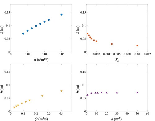
Water depth is an important parameter to characterize the shallowness of an open water body, considering a fixed-width channel (B = 1.2 m). An open flow with an aspect ratio defined by channel width divided by water depth greater than 5 is known as shallow water flow. From the simulated results, the aspect ratio ranges from 8.46-81.6 across all simulated scenarios, corresponding to a water depth of 0.14-0.015 m. Previous studies demonstrated that the shallowness of flow significantly influences the growth of the mixing layer, which before examining the mixing shear characteristics requires an initial assessment of water depth variation in response to changed values of the selected controlled factors (Figure 2). Clearly, the water depth varies monotonously with the controlling factors. Specifically, water depth grows with the increase in manning coefficient (n), water discharge (Q) and canopy density (a), but decreases with the increase in bed slope (S_b). It should be noted that the variation range of water depth is sensitive to the value change of factors, except for scenarios of changing canopy density, which is counterintuitive and to our knowledge is not reported by other studies. Therefore, solely changing canopy density might be not essential to the growth of PCFs-type mixing layers due to insignificant changes in water shallowness.

Figure 2. Water depth influenced by changing values of the factors.

3.2. Lateral distribution of the mean flow

For partially-distributed canopy flows (PCFs), a two-layer mean flow structure including the lateral distribution of longitudinal flow velocity and Reynolds shear stress across the inner layer (canopy side) and outer layer (non-canopy side) is a hydrodynamic signature. Figure 3 shows the variation of the lateral distribution of the mean flow influenced by changed controlled factors, which can well account for the vortex fields in the previous section. For the mean velocity, it is interesting that for the changed manning coefficient and water discharge, the constant velocity in the inner layer remains unchanged as the factors increase in magnitude. This is mainly because with the same bed slope and canopy density, the inner-layer velocity is developed to contribute the balance between canopy drag and gravitational force (1/2C_daU₁²= gS_b and U₁= (2gS_b/C_da)^1/2). According to the momentum balance, the increase in bed slope or decrease in canopy density can lead to an increase in the constant inner-layer velocity, which is well illustrated in Figure 3b,d. Moreover, the variation of U₁ is not pronounced for high canopy densities due to the inverse association. For example, the velocity difference between a = 9 and 50m⁻¹ is ∼0.015 m/s, which corresponds to the difference of ∼ 0.027 m/s between a = 1 and 5m⁻¹.

Figure 3. Lateral profiles of (a) longtidinal velocity U and (b) Reynolds shear stress τ_xy influenced by the factors.

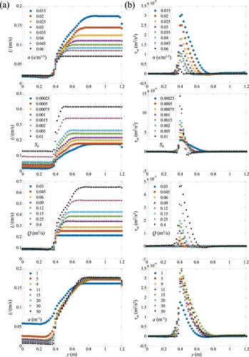
The constant outer-layer velocity varies soundly nearly for all controlled factors being changed, except for canopy density. The momentum balance for fully-developed flows in the absence of vegetation canopy has gS_bh = 1/2c_fU₂² with c_f= gn²/h^1/3, yielding U₂= (2S_bh^4/3/n²)^0.5. First, the constant outer-layer velocity decreases consistently with the growing manning coefficient. Although the water depth plays a positive role in the manning relationship, the bed friction seems to contribute more to determining the velocity. It can be seen that the outer layer dominates the growth of the lateral shear mixing. With the decrease in the outer-layer velocity due to the increasing manning coefficient, the mixing layer width also decreases. Water discharge works quite similarly to the manning coefficient but in an opposite way. A higher water discharge produces a larger constant outer-layer velocity and mixing shear width. This might be interpreted in a way that the water depth.

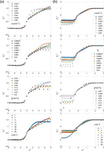
Similarity essentially exists in the lateral profiles of longitudinal velocity and Reynolds shear stress in shallow mixing layers, suggesting the scalability of these lateral profiles (Proust et al., 2017). Also, with proper lengths, PCFs conform to similarity due to the nature of shallow mixing layers (White & Nepf, 2007, 2008). However, such similarity has not been examined when the stabilization effect on the mixing layer is significant. Here, we present the scaling for the longitudinal velocity. For the inner layer (canopy zone), the inner length scale of the mixing layer controls the shape of the lateral profiles. Based on the delineation of the structure of the mixing layer (White & Nepf, 2007), the length scales respective to the inner and outer layers are calculated as characteristic velocity differences divided by the velocity gradient for the corresponding sub-layers, respectively. Specifically, the inner-layer characteristic velocity difference is U_ed-U₁, with the velocity inflection point simply assumedly coincident with the canopy edge; and the outer-layer characteristic velocity difference is U₂-U_m, where U_m is the velocity of the velocity gradient match point between the inner layer and outer layer. Thus, we have δ_i= (U_ed-U₁)/(dU/dy|_yed) and δ_o= (U₂-U_m)/(dU/dy|_ym).

Figure 4 shows the results of scaled lateral profiles of longitudinal velocity for the inner layer [U_i* = (U-U₁)/(U_ed-U₁)/2 and y_i* = (y-y_ed)/δ_i] and outer layer [U_o* = (U₂-U)/(U₂-U_m)/2 and (y-y_m)/δ_o]for different scenarios. It can be observed that under different influences, the inner-layer profiles and outer-layer profiles of scaled longitudinal velocity well collapse onto universal curves for the two sub-layers. However, we can also find that the scaled profiles of longitudinal velocity cannot be completely universal regarding either the inner length scale or the outer length scale. This is owing to the asymmetry of the shallow mixing layers in PCFs, differing from splitter plate or compound channel flows (Proust et al., 2017; Proust et al., 2022).

Figure 4. Two-layer similarity in the lateral profiles of longtidinal velocity U regarding (a) inner length scale and (b) outer length scale.

3.3. Oscillating vortex fields

The vortex fields of fully developed flows for PCFs influenced by different controlled factors are illustrated in Figure 5. By fixing other input parameters, one controlled factor is changed gradually to observe the responding simulated results. First, we examine the effect of bed roughness indicated by the manning coefficient (n) on the vortex fields (Figure 5a). It is intrusive that higher bed roughness tends to resist and stabilize flow motion. As a result, the horizontal scales (length and width) of canopy-scale vortices decay with increasing manning coefficient. With one window, the number of vortex circulation (indicated by concentrated vorticity) effectively increases. Particularly, we can claim that the vortex transforms into something like perturbations along the lateral edges. However, a larger manning coefficient, with other parameters being constant (e.g. water discharge, energy slope and canopy density), can also promote the increase in water depth, which might destabilize the flow motion due to the weakened shallowness effect. Therefore, it can be said that the enhanced bed friction effect outperforms the weakened shallowness effect with an increase in the manning coefficient that characterizes bed roughness.

Figure 5. Oscillating vortex fields for PCFs influenced by the factors.

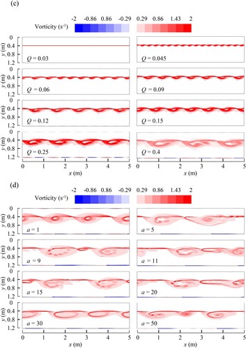
Figure 5b shows the spatial pattern of vortex fields for changed bed slope (S_b). Similar to the manning coefficient, with an increasing bed slope, the horizontal scales of the vortex are likely to decay. The magnitude of vorticity tends to increase as the bed slope increases, which differs from the effect of increasing the manning coefficient indicated by insignificant varied vorticity. This difference is due to the shear extent near the lateral canopy edge. Increasing bed slope with a constant water discharge, manning coefficient and canopy density, results in decreasing water depth (or enhanced shallowness) but increasing velocity difference between the canopy side and non-canopy side that might induce Kelvin-Helmholtz flow instability. Therefore, increasing bed slope through enhancing the shallowness effect destabilizes the canopy-scale vortices effectively.

Then, the effect of increasing water discharge (Figure 5c) is examined with a relatively high bed slope (S_b= 0.005), which inherently tends to impose a stabilization effect on large vortex growth. Solely increasing mass flux with other controlled factors fixed not only strengthens the lateral shear but also promotes the increase in water depth (or weakens shallowness). Such two tendencies are understood to feed positive back to the growth of horizontal vortices. The results rationally support the above understanding by showing that both the amplitude and wavelength of the vortex structure increase for a higher water discharge.

As for canopy density (Figure 5d), it essentially controls the division of mass and momentum of canopy side and non-canopy side. The simulated results show that as the canopy density gradually increases, the scale variation of vortices is insignificant compared with other factors. It can be concluded the vortex length (or wavelength) becomes slightly smaller for the lowest and highest canopy density, which is indicated by more vortex circulation with the same referenced sampling window. However, the lateral penetration of the vortices tends to be enhanced as canopy density decreases. This consistently agrees with previous experimental studies (Nepf, 2012; White & Nepf, 2008). A noticeable case is that for the lowest canopy density (a = 1m⁻¹), the penetration length (or inner length) of a vortex becomes comparable to the outer length, while the latter far exceeds the former as canopy density increases. The results suggest that canopy density might be not important to vortex growth but important to the lateral alignment of the vortex. As suggested previously (Nepf, 2012), horizontal canopy-scale vortices occur for ah > 0.1. However, vortices are also triggered when ah = 0.067. This inconsistency might be owing to the experimental measurement difficulty of vortices under a very small canopy density.

4. Discussion

4.1. Characterisc scales

The proceeding evaluations of mean flow and vortex fields in various scenarios of changing influential factors suggested that the growth of turbulent mixing layers in PCFs is suppressed due to either increasing bed friction or enhancing water shallowness. This is consistent with the knowledge previously gained from classic shallow mixing layers such as splitter plate flows and compound channel flows (Chu & Babarutsi, 1988; Ghidaoui & Kolyshkin, 1999). Differing from such classic shallow mixing shears whose extents on the slow- and fast- flow sides are equal, the inner and outer parts of the mixing layer in PCFs are commonly asymmetric. The inner is far smaller than the outer due to the presence of the canopy drag, except for the scenario of the smallest canopy density (a = 1m⁻¹) (Figure 5). Therefore, a mixing layer in PCFs against the canopy edge is suggested to own inner- and outer-layer length scales, in addition to a full-length scale as their sum. Additionally, the constant velocity difference across the mixing layer and the maximum Reynolds shear stress can be used to account for the velocity scales, which are consistent with classic studies of shallow mixing layers (Chu & Babarutsi, 1988; White & Nepf, 2007).

Figure 6 shows the behaviour of the velocity scales and length scales in PCFs vary with the changed value of influential factors. Nearly all the characteristic scales vary monotonously with the factors, except for 2(τ_xy)^1/2/(U₁+ U₂) at the small-value range of manning coefficient and bed slope. Generally, the six scale parameters decrease with the increase in manning coefficient and bed slope, and increase with the increase in water discharge. As shown previously, increasing the manning coefficient and bed slope tends to stabilize the flow in the mixing shear layer as indicated by smaller-scale vortices in one computational domain (Figure 5). Regarding n and S_b, the significant decay of length scales (δ_i, δ_o, δ_i+ δ_o) corresponds to the dimensionless velocity difference [2(U₂-U₁)/(U₁+ U₂)] approaching 1 when the significant destabilization of the flow. This approaching-to-one phenomenon can be found for smaller water discharge and canopy density as well, under which the vortex is not significantly triggered. The causes accounting for the decrease in 2(U₂-U₁)/(U₁+ U₂) regarding the two factors, however, are inconsistent. All characteristic velocities [U₁, U₂ and (U₁+ U₂)/2] decrease for increasing n while increasing for increasing S_b, which correspond to increase and decrease in water depth, respectively. Therefore, either bed friction or water shallowness cannot solely determine whether the mixing layer in PCFs grows or not. According to the current results, an in-depth analyzed factor, e.g. the dimensionless velocity difference, seems a good indicative candidate, which unfortunately is indirectly obtained. In addition, the decrease in the length scales performs a linear trend for n, which differs from the exponential decay trend for S_b. This on the other hand also demonstrates that the destabilization effect between increasing n and S_b might be distinct.

Figure 6. Dependence of characteristic scales of shallow mixing layers in PCFs (velocity scales [2(U₂-U₁)/(U₁+ U₂) and 2(τ_xy)^1/2/(U₁+ U₂)] and length scales [δ_i, δ_o, δ_i+ δ_o and δ_o/δ_i]) on the influential factors.

The increase in water discharge, clearly, tends to enhance the flow instability, indicated by the increase in both velocity scales and length scales (Figure 6). With a larger water discharge, a freer confinement environment for the vortex growth is created due to both larger water depth and characteristic velocities. Differing from conventional shallow mixing layers, the canopy layer can impose resistance to avoid the further expansion of the vortices on the slow-speed canopy side. As canopy density increases, the dimensionless velocity difference and Reynolds shear stress monotonously increase, while the inner length decreases. Notably, the outer length initially increases till a = 15m⁻¹ and then decreases for larger density despite larger dimensionless velocity difference and Reynolds shear stress. The vortex shrink behaviour due to the increasing canopy denseness has been reported in vertically-circulated vortices in submerged canopy flows by Poggi et al. (2004) and Nepf (2012). The essential mechanism is that the shear production of feeding energy into the vortices should be balanced by the dissipation of the canopy drag as explained by Nepf (2012). When the canopy is sufficiently dense, the canopy drag may reduce as the stem wakes cannot be fully developed due to the stem sheltering effect (X), such that the reached vortex scale is also suppressed. This might be well understood with an extreme scenario that which an extremely dense canopy layer behaves like a solid wall, above which a smaller-scale wall-detached structure is generated.

The ratio of inner length to outer length (δ_o/δ_i) indicates the symmetric extent of the mixing layer. The mixing layer tends to be less asymmetric as indicated by decreasing δ_o/δ_i, as the manning coefficient and bed slope increase and the discharge decreases. This is consistent with the tendency of destabilizing canopy-scale vortices. A lower canopy density can also produce less asymmetry of vortices without reducing significantly the scales of inner and outer layers, which is due to that the reduced canopy drag allows more momentum penetration.

The influential factors soundly determine the quantities of characteristic scales (i.e. velocity scales and length scales) of mixing layers for PCFs, which is well addressed by changing one while fixing others. To quantify these effects, a parameter ($\mathrm{Se}=\frac{c_f}{2h}\frac{U_m}{\mathrm{\Delta }U}$) which has the reversal dimension of a length scale is used for evaluating the dependency relation. This parameter originates from the dimensionless bed friction parameter $S=\frac{c_f\delta }{2h}\frac{U_m}{\mathrm{\Delta }U}$, which for conventional mixing layers (splitter plate flows and compound channel flows) is used to evaluate the destabilization effect of bed friction and water shallowness. Therefore, Se can be interpreted as the stabilization efficiency on average over the entire mixing layer. Because the velocity difference of mixing layer is incorporated into this parameter, we only address length scales here.

Figure 7 shows the dependency relationship between the characteristic scales (velocity scales [2(U₂-U₁)/(U₁+ U₂) and 2(τ_xy)^1/2/(U₁+ U₂)] and length scales [δ_i, δ_o, δ_i+ δ_o and δ_o/δ_i]) and stabilization efficiency parameter Se. It can be observed that all characteristic scales well depend on the proposed stabilization efficiency parameter Se. 2(U₂-U₁)/(U₁+ U₂) decreases with Se, which can be fitted by a negative logarithmic function with the correlation attaining R²= 0.96. 2(τ_xy)^1/2/(U₁+ U₂) is shown to have negative linear dependence with S_e, with a lower correlation R²= 0.9 compared with the velocity. All length scales (δ_i, δ_o and δ_i+δ_o) decrease as the stabilization efficiency parameter (Se) increases, indicating that the mixing layers for PCFs tend to be stable with the enhanced combined effect of bed friction and water shallowness. Interestingly, the ratio of outer length to inner length (δ_o/δ_i) also decreases with S_e, indicating that with higher stabilization efficiency the mixing layer becomes narrower but more symmetric. This in turn suggests that the outer part of the mixing layer is easier to be disturbed than the inner part does, which is essentially attributed to the constraint arising from canopy drag. Expect the inner length scale regarding the variation of canopy density, all length scales and scale ratio nearly collapse onto universal curves of exponential decay function with the fitting correlation R²= 0.79 and above. The data of the inner length scale under different canopy densities sets a standalone trend, which differs from the outer length scale. Since the outer length scale dominates the width of the mixing layer for most scenarios of high canopy density (see Figure 5), the width of the mixing layer and the scale ratio of outer to inner length can also follow the fitting curve for all influential factors including canopy density. We reasonably speculate that a certain canopy density owns a certain fitting curve for the inner length with variable bed friction and water shallowness.

Figure 7. Dependence of characteristic scales (velocity scales [2(U₂-U₁)/(U₁+ U₂) and 2(τ_xy)^1/2/(U₁+ U₂)] and length scales [δ_i, δ_o, δ_i+ δ_o and δ_o/δ_i]) on stabilization efficiency parameter (Se).

There exists a standalone dependency of the inner length scale on the stabilization efficiency parameter Se regarding the scenario of changing canopy density. Increasing canopy density negligibly influences bed friction and water shallowness but enhances the interface shear. These combined effects lead to the reduction of stabilization efficiency parameter Se. However, the inner length does not correspondingly increase, which suggests that the conventional concept of stabilization effect does not apply to the canopy layer and the canopy drag plays a negative role in the growth of the inner part of the mixing layer.

The product of the stabilization efficiency parameter (Se) and mixing layer width (δ_i+δ_o) yields the bed friction parameter, which can indicate the stability regime of shallow mixing layers. For splitter plate flows, Chu and Babarutsi (1988) suggested that with the parameter smaller than 0.09, the mixing layer became unstable. For all modelling scenarios in this work, S = Se(δ_i+δ_o) ranges from 0.0042 to 0.03, with the flow of the maximum-value case (S = 0.03) is stable (see Figure 5c). Therefore, it is suggested that mixing layers in PCFs are harder to be destabilized due to the presence of the canopy resistance compared with other mixing layer flows.

4.2. Wave periodicity

The periodicity of the horizontal large-scale vortices is also a fundamental property that needs to draw particular attention, which can guide the practical sampling of the real-world fluctuating velocities. Following Jia et al., (2022), wavelength (λ) is estimated as the averaged distance between neighbouring vortices over at least 10 cycles after the flow is fully developed, while wavenumber (k) is calculated based on the inherent relation k = 2π/λ. Therefore, a greater wavelength means a lower wavenumber, which suggests the larger scales of interface vortices.

Figure 8 shows the dependence of wavelength and wavenumber on individual influential factors. Similar to the characteristic length scales, the wavelength decreases with increasing manning coefficient or bed slope and increases with increasing water discharge, suggesting that the horizontal large-scale vortices grow in lateral and longitudinal directions, simultaneously. Wavenumber, correspondingly, presents the opposite behaviour. Regarding the effect of canopy density, the wavelength nearly remains constant except for the smallest and largest densities, which is similar to the variation of outer length. Thus, the wavenumber nearly remains at a constant lower level compared with the other three scenarios. This is because the change in canopy density imposes a negligible stabilization effect on the mixing layer.

Figure 8. Dependence of wavelength (λ) and wavenumber (k) of oscillating horizontal canopy-scale vortices in PCFs on the influential factors.

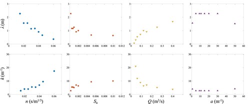
Figure 9 shows the scaling characteristics of the periodicity of horizontal large-scale vortices against the stabilization efficiency parameter (Se). In consistency with the lateral length scales (particularly the outer length and full length), the wavelength also decays with the increase in S_e, fitted with an exponential decay function (R²= 0.91). The wavenumber, however, can be scaled by a linear function of Se (R²= 0.87). Larger biases occur for larger SL, at which the flow tends to be stabilized by the combined effect of bed friction and water shallowness. This might be attributed to amplified statistical errors when coping with small-scale eddies.

Figure 9. Dependence of (a) wavelength (λ) and (b) wavenumber (k) of oscillating horizontal canopy-scale vortices in PCFs on the stabilization efficiency parameter (Se) and (c) wavelength on the width of mixing layer.

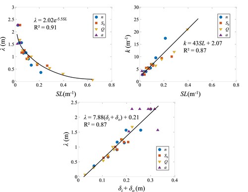
Also, we present the comparison between the lateral length and wavelength, which can imply the full planar geometric shape of horizontal vortices. It can be generally concluded that the longitudinal length of horizontal vortices greatly outweighs the lateral length by over five times, indicating the horizontal vortices are elongated for PCFs. The elongation of large-scale vortices for PCFs differs from the comparable lateral and longitudinal scales for shallow mixing layers for parallel and non-parallel streams in far fields (Cheng & Constantinescu, 2020, 2021) and is similar to the scenarios for floodplain flows (Van Prooijen et al., 2000). Based on the continuity principle, this highly anisotropic property suggests that the intensity of streamwise fluctuations becomes far greater than the lateral fluctuations. The planar geometric shape of horizontal vortices is self-similar across a wide range of flow configurations. The similarity can be described by a linear function between the lateral length and longitudinal length, i.e. λ = 7.88(δ_i+δ_o) + 0.21 with R²= 0.87. The exception again occurs for the scenarios of changing canopy density, which can be explainable that the inner length of the mixing layer becomes larger when the canopy is sparser with the outer length changing slightly.

4.3. Implications and limitations

The colonization of vegetation across the bed is shown to trigger horizontal oscillation motions along the junction between the main channel (non-canopy zone) and flow-retarded channel (canopy zone), inherently similar to other natural shallow mixing layers. Under a certain canopy configuration, the mixing behaviour for PCFs follows consistently that for typical shallow mixing layers, the bed friction and water shallowness are able to stabilize oscillating flow motion and suppress the mixing processes. Unlikely, the denseness (or porosity) of the canopy plays a significant role in mediating the inner (canopy-side) mixing processes, essentially differing from other types. A denser canopy leads to more outward-asymmetric horizontal vortices so that transversely-transport scalar (such as suspended sediment and plant seeds) is somehow limited to the margin of the canopy. This may account for why elongated patches of pioneering vegetation are often found to occur on bar margins (Asaeda et al., 2010; Zhou et al., 2018). Thus, a conceptual model can be concluded to describe the shallow mixing shear caused large-scale vortex system in PCFs as shown in Figure 10.

Figure 10. Conceptual model of shallow mixing shear caused large-scale vortex system in PCFs mediated by canopy denseness, flow shallowness and bed friction. The change in the various effects is indicated by the darkening and lightening of the colours.

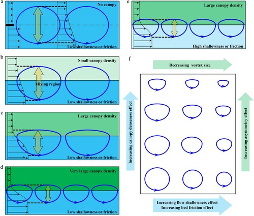
For a splitter plate shallow mixing layer, nearly symmetric KH vortices are developed due to the initial differential velocity profile (Figure 10a). When a sparse canopy is present partially on the bed with negligible bed effect (friction and shallowness effects), KH vortices are able to be triggered and maintained by the porous canopy-caused differential velocity profile. However, due to the canopy drag, the inner part of the vortices is not fully developed compared with the counterpart in the main channel, leading to an asymmetric distorted vortex system. This geometry distortion is facilitated by the increasing canopy denseness effect (Figure 10b). It can be expected that the sufficiently high canopy denseness can suppress the growth of the vortex system with the wave number increasing. Regarding the bed effect, either high shallowness or friction plays a role in stabilizing the shallow mixing layers (with smaller vortex scales), which is similar to other shallow mixing layers. Owing to the canopy porosity, the threshold of the bed frictional parameter triggering the instability of shallow mixing layers in PCFs becomes lower compared with other non-vegetated shallow mixing layers, indicating a more stable flow field. Therefore, a comprehensive understanding can be achieved that a particular denseness configuration of canopy sets up channel planform for shallow mixing layer development, which can follow a universal mixing asymptotic behaviour affected by bed friction and water shallowness. The variation of canopy denseness, however, encourages another mixing asymptotic behaviour by only shifting the basic one. Figure 10e summarizes the above processes with a simple schematic phenomenological model.

Our results can be applicable to nearly all scenarios of the PCFs with a vertically uniform canopy density of about a = 9m⁻¹. The current results cannot be generalized particularly for variable canopy densities due to a lack of sufficient experimental and numerical data analysis. By changing canopy density while fixing other factors, the results can provide new insights into the role of the near-bank canopy in medicating the mixing behaviour for PCFs in contrast to other typical shallow mixing layers.

Another concern is that the results are based on two-dimensional shallow open water equations. Although for the condition of PCFs, the horizontal length scale overwhelms the vertical counterpart, the recent three-dimensional experimental works (Yan et al., 2022a; Yan et al., 2023) revealed that the junctional flow is obviously three-dimensional both for submerged and emergent conditions due to turbulence anisotropy produced by multiple (solid or porous) boundaries. Despite good agreement between the modelled transverse profiles of depth-averaged flow velocity and Reynolds shear stress and the observed data, we cannot be ascertain that the depth-averaged modelling is consistently reasonable when the influence of bed friction and water shallowness is significant. Our results, therefore, are suggested to be further confirmed by sophisticated results from three-dimensional numerical modelling or experiment observation.

5. Conclusions

In recent decades, hydrodynamics, sediment transport and solute dispersion in partially-distributed canopy flows (PCFs) or similarly-configured flows have been discussed heatedly for understanding fluvial processes, promoting environmental preservation and mitigating flood hazards. Previous documents gain numerous conclusions with weak consideration of the effects of bed friction and water shallowness, which exert a stabilization effect on oscillating flow motion across the lateral interface of the canopy. This may set uncertainty to the application of relevant theory. To address this issue, depth-averaged Large Eddy Simulation (DA-LES) is used to model PCFs to provide fundamental data for evaluating shallow mixing layers under the variation of bed friction, water shallowness and canopy denseness. The main conclusions are drawn in the following,

1. The influence of bed friction, water shallowness and canopy denseness is produced by changing manning coefficient, bed slope and water discharge and canopy density. The transverse profile of time-mean depth-averaged flow velocity and Reynolds shear stress mediated by the influential factors follows the scaling behaviour subjected to shallow mixing layers. The presence of canopy drag, however, limits the further lateral extension of the mixing layer into the canopy, requiring the scaling length scale for the mixing-layer-type distribution to be consistent with the inner and outer parts of the mixing layers.

2. In contrast to typical shallow mixing layers (splitter plate flows and compound channel flows), the mixing layers in PCFs tend to be highly asymmetric. This is because the outer part can be freely disturbed while the inner part is highly constrained by the canopy drag. The asymmetry effect of mixing layers is weakened as canopy denseness decreases as well as bed friction and water shallowness are more felt.

3. Characteristic scales of shallow mixing layers in PCFs are found to be similar regarding a stabilization efficiency parameter, which can be delineated by exponential decay functions. The variation of canopy denseness, however, sets the scales associated with the inner part of the mixing layer to bias from the similarity, and it plays a role in making an overall shift of characteristic scale similarity in mixing layers for a broad range of bed friction and water shallowness.

4. The bed friction parameter thresholding (about 0.03) in PCFs is lower than compared with other shallow mixing layers (e.g. about 0.09 for splitter plate flows). It is inferred that the partially-distributed canopy tends to inhibit the instability of the shallow mixing layers in PCFs. Finally, we propose a conceptual model of describing the hydrodynamic behaviour and vortex system of PCFs-caused shallow mixing layers.

Disclosure statement

No potential conflict of interest was reported by the author(s).

Data availability

Data will be made available on request.

Additional information

Funding

This research was supported by the Open Research Fund of State Key Laboratory of Simulation and Regulation of Water Cycle in River Basin, China Institute of Water Resources and Hydropower Research, Grant NO. IWHR-SKL-KF202320, College Students’ Innovative Entrepreneurial Training Plan Program (C2023127033, C2024129167).

References

- Anderson, B. G., Rutherfurd, I. D., & Western, A. W. (2006). An analysis of the influence of riparian vegetation on the propagation of flood waves. Environmental Modelling & Software, 21, 1290–1296. https://doi.org/10.1016/j.envsoft.2005.04.027
- Asaeda, T., Gomes, P. I., & Takeda, E. (2010). Spatial and temporal tree colonization in a midstream sediment bar and the mechanisms governing tree mortality during a flood event. River Research and Applications, 26, 960–976. https://doi.org/10.1002/rra.1313
- Ben Meftah, M., De Serio, F., & Mossa, M. (2014). Hydrodynamic behavior in the outer shear layer of partly obstructed open channels. Physics of Fluids, 26, 065102. https://doi.org/10.1063/1.4881425
- Chen, W. Y., & Cho, F. H. T. (2019). Environmental information disclosure and societal preferences for urban river restoration: Latent class modelling of a discrete-choice experiment. Journal of Cleaner Production, 231, 1294–1306. https://doi.org/10.1016/j.jclepro.2019.05.307
- Cheng, Z., & Constantinescu, G. (2020). Near-and far-field structure of shallow mixing layers between parallel streams. Journal of Fluid Mechanics, 904, A21. https://doi.org/10.1017/jfm.2020.638
- Cheng, Z., & Constantinescu, G. (2021). Shallow mixing layers between non-parallel streams in a flat-bed wide channel. Journal of Fluid Mechanics, 916. https://doi.org/10.1017/jfm.2021.254
- Chu, V. H., & Babarutsi, S. (1988). Confinement and bed-friction effects in shallow turbulent mixing layers. Journal of Hydraulic Engineering, 114, 1257–1274. https://doi.org/10.1061/(ASCE)0733-9429(1988)114:10(1257)
- de Lima, A., & Izumi, N. (2014). On the nonlinear development of shear layers in partially vegetated channels. Physics of Fluids, 26, 084109. https://doi.org/10.1063/1.4893676
- Duan, J. G., & Nanda, S. K. (2006). Two-dimensional depth-averaged model simulation of suspended sediment concentration distribution in a groyne field. Journal of Hydrology, 327, 426–437. https://doi.org/10.1016/j.jhydrol.2005.11.055
- Elder, J. (1959). The dispersion of marked fluid in turbulent shear flow. Journal of Fluid Mechanics, 5, 544–560. https://doi.org/10.1017/S0022112059000374
- Ghidaoui, M. S., & Kolyshkin, A. A. (1999). Linear stability analysis of lateral motions in compound open channels. Journal of Hydraulic Engineering, 125, 871–880. https://doi.org/10.1061/(ASCE)0733-9429(1999)125:8(871)
- Guo, J., Jiang, W., & Chen, G. (2020). Transient solute dispersion in wetland flows with submerged vegetation: An analytical study in terms of time-dependent properties. Water Resources Research, 56, e2019WR025586.
- Gurnell, A. (2014). Plants as river system engineers. Earth Surface Processes and Landforms, 39, 4–25. https://doi.org/10.1002/esp.3397
- Gurnell, A. M., Petts, G. E., Hannah, D. M., Smith, B. P., Edwards, P. J., Kollmann, J., & Tockner, J. V. W. (2001). Riparian vegetation and island formation along the gravel-bed Fiume Tagliamento, Italy. Earth Surface Processes and Landforms: The Journal of the British Geomorphological Research Group, 26, 31–62.
- Hinterberger, C., Fröhlich, J., & Rodi, W. (2007). Three-dimensional and depth-averaged large-eddy simulations of some shallow water flows. Journal of Hydraulic Engineering, 133, 857–872. https://doi.org/10.1061/(ASCE)0733-9429(2007)133:8(857)
- Huai, W., Xue, W., & Qian, Z. (2015). Large-eddy simulation of turbulent rectangular open-channel flow with an emergent rigid vegetation patch. Advances in Water Resources, 80, 30–42. https://doi.org/10.1016/j.advwatres.2015.03.006
- Jang, C.-L., & Shimizu, Y. (2005). Numerical simulation of relatively wide, shallow channels with erodible banks. Journal of Hydraulic Engineering, 131, 565–575. https://doi.org/10.1061/(ASCE)0733-9429(2005)131:7(565)
- Jang, C.-L., & Shimizu, Y. (2007). Vegetation effects on the morphological behavior of alluvial channels. Journal of Hydraulic Research, 45, 763–772. https://doi.org/10.1080/00221686.2007.9521814
- Jia, Y.-Y., Yao, Z.-D., Duan, H.-F., Wang, X.-K., & Yan, X.-F. (2022). Numerical assessment of canopy blocking effect on partly-obstructed channel flows: From perturbations to vortices. Engineering Applications of Computational Fluid Mechanics, 16, 1761–1780. https://doi.org/10.1080/19942060.2022.2109757
- Kasvi, E., Alho, P., Lotsari, E., Wang, Y., Kukko, A., Hyyppä, H., et al. (2015). Two-dimensional and three-dimensional computational models in hydrodynamic and morphodynamic reconstructions of a river bend: sensitivity and functionality. Hydrological Processes, 29, 1604–1629. https://doi.org/10.1002/hyp.10277
- Koken, M., & Constantinescu, G. (2023). Influence of submergence ratio on flow and drag forces generated by a long rectangular array of rigid cylinders at the sidewall of an open channel. Journal of Fluid Mechanics, 966, A5. https://doi.org/10.1017/jfm.2023.427
- Lazzarin, T., & Viero, D. P. (2023). Curvature-induced secondary flow in 2D depth-averaged hydro-morphodynamic models: An assessment of different approaches and key factors. Advances in Water Resources, 171. https://doi.org/10.1016/j.advwatres.2022.104355
- Li, C. W., & Zhang, M. (2010). Numerical modeling of shallow water flow around arrays of emerged cylinders. Journal of Hydro-Environment Research, 4, 115–121. https://doi.org/10.1016/j.jher.2010.04.005
- Li, J., Claude, N., Tassi, P., Cordier, F., Crosato, A., & Rodrigues, S. (2023). River restoration works design based on the study of early-stage vegetation development and alternate bar dynamics. River Research and Applications, 39(9), 1682–1695.
- Lima, A., & Izumi, N. (2011). Instability of shallow open channel flow with lateral velocity gradients. Journal of Physics: Conference Series. 318. IOP Publishing, pp. 032002. https://doi.org/10.1088/1742-6596/318/3/032002
- Liu, C., & Shan, Y. (2019). Analytical model for predicting the longitudinal profiles of velocities in a channel with a model vegetation patch. Journal of Hydrology, 576, 561–574. https://doi.org/10.1016/j.jhydrol.2019.06.076
- Liu, M., Yang, Z., Ji, B., Huai, W., & Tang, H. (2022). Flow dynamics in lateral vegetation cavities constructed by an array of emergent vegetation patches along the open-channel bank. Physics of Fluids, 34, 035122.
- Lloyd, P. M., & Stansby, P. K. (1997). Shallow-water flow around Model Conical Islands of Small Side Slope. II: Submerged. Journal of Hydraulic Engineering, 123(12), 1057–1067.
- Meftah, M. B., & Mossa, M. (2016). Partially obstructed channel: Contraction ratio effect on the flow hydrodynamic structure and prediction of the transversal mean velocity profile. Journal of Hydrology, 542, 87–100. https://doi.org/10.1016/j.jhydrol.2016.08.057
- Molls, T., & Chaudhry, M. H. (1995). Depth-averaged open-channel flow model. Journal of Hydraulic Engineering, 121, 453–465. https://doi.org/10.1061/(ASCE)0733-9429(1995)121:6(453)
- Nadaoka, K., & Yagi, H. (1998). Shallow-water turbulence modeling and horizontal large-eddy computation of river flow. Journal of Hydraulic Engineering, 124, 493–500. https://doi.org/10.1061/(ASCE)0733-9429(1998)124:5(493)
- Nepf, H. M. (2012). Hydrodynamics of vegetated channels. Journal of Hydraulic Research, 50, 262–279. https://doi.org/10.1080/00221686.2012.696559
- Nezu, I., & Onitsuka, K. (2001). Turbulent structures in partly vegetated open-channel flows with LDA and PI V measurements. Journal of Hydraulic Research, 39, 629–642. https://doi.org/10.1080/00221686.2001.9628292
- Poggi, D., Katul, G., & Albertson, J. (2004). A note on the contribution of dispersive fluxes to momentum transfer within canopies. Boundary-Layer Meteorology, 111, 615–621. https://doi.org/10.1023/B:BOUN.0000016563.76874.47
- Proust, S., Berni, C., & Nikora, V. I. (2022). Shallow mixing layers over hydraulically smooth bottom in a tilted open channel. Journal of Fluid Mechanics, 951, A17. https://doi.org/10.1017/jfm.2022.818
- Proust, S., Fernandes, J. N., Leal, J. B., Rivière, N., & Peltier, Y. (2017). Mixing layer and coherent structures in compound channel flows: Effects of transverse flow, velocity ratio, and vertical confinement. Water resources research, 53, 3387–3406. https://doi.org/10.1002/2016WR019873
- Su, X., & Li, C. W. (2002). Large eddy simulation of free surface turbulent flow in partly vegetated open channels. International Journal for Numerical Methods in Fluids, 39, 919–937. https://doi.org/10.1002/fld.352
- Van Prooijen, B., Booij, R., & Uijttewaal, W. (2000). Measurement and analysis methods of large scale horizontal coherent structures in a wide shallow channel. 10th international Symposium on Applications of Laser Techniques to Fluid Mechanics, Calouste Gulbenkian Foundation, Lisbon, Portugal.
- van Zelst, V. T., Dijkstra, J. T., van Wesenbeeck, B. K., Eilander, D., Morris, E. P., Winsemius, H. C., Ward, P. J., & de Vries, M. B. (2021). Cutting the costs of coastal protection by integrating vegetation in flood defences. Nature Communications, 12, 6533. https://doi.org/10.1038/s41467-021-26887-4
- White, B. L., & Nepf, H. M. (2007). Shear instability and coherent structures in shallow flow adjacent to a porous layer. Journal of Fluid Mechanics, 593, 1–32. https://doi.org/10.1017/S0022112007008415
- White, B. L., & Nepf, H. M. (2008). A vortex-based model of velocity and shear stress in a partially vegetated shallow channel. Water Resources Research, 44. https://doi.org/10.1029/2006WR005651
- Wu, W. (2004). Depth-averaged two-dimensional numerical modeling of unsteady flow and nonuniform sediment transport in open channels. Journal of Hydraulic Engineering, 130, 1013–1024. https://doi.org/10.1061/(ASCE)0733-9429(2004)130:10(1013)
- Xie, Z., Lin, B., & Falconer, R. A. (2013). Large-eddy simulation of the turbulent structure in compound open-channel flows. Advances in Water Resources, 53, 66–75. https://doi.org/10.1016/j.advwatres.2012.10.009
- Xu, Z.-X., Ye, C., Zhang, Y.-Y., Wang, X.-K., & Yan, X.-F. (2020). 2D numerical analysis of the influence of near-bank vegetation patches on the bed morphological adjustment. Environmental Fluid Mechanics, 1–32. https://doi.org/10.1007/s10652-019-09718-5
- Yan, X.-F., Duan, H.-F., Wai, W.-H. O., Li, C.-W., & Wang, X.-K. (2022a). Spatial flow pattern, multi-dimensional vortices and junction momentum exchange in a partially-covered submerged canopy flume. Water Resources Research, 58, e2020WR029494. https://doi.org/10.1029/2020WR029494
- Yan, X. F., Duan, H. F., Yang, Q. Y., Liu, T. H., Sun, Y., & Wang, X. K. (2022b). Numerical assessments of bed morphological evolution in mountain river confluences under effects of hydro-morphological factors. Hydrological Processes, 36, e14488. https://doi.org/10.1002/hyp.14488
- Yan, X. F., Jia, Y. Y., Zhang, Y., Fang, L. B., Duan, H. F., & Wang, X. K. (2023). Hydrodynamic adjustment subject to a submerged canopy partially obstructing a flume: Implications for junction flow behavior. Ecohydrology, e2467. https://doi.org/10.1002/eco.2467
- Yan, X.-F., Wai, W.-H. O., & Li, C.-W. (2016). Characteristics of flow structure of free-surface flow in a partly obstructed open channel with vegetation patch. Environmental Fluid Mechanics, 16, 807–832. https://doi.org/10.1007/s10652-016-9453-4
- Yang, K., Nie, R., Liu, X., & Cao, S. (2013). Modeling depth-averaged velocity and boundary shear stress in rectangular compound channels with secondary flows. Journal of Hydraulic Engineering, 139, 76–83. https://doi.org/10.1061/(ASCE)HY.1943-7900.0000638
- Zhang, Y.-H., Duan, H.-F., Yan, X.-F., & Stocchino, A. (2023). Experimental study on the combined effects of patch density and elongation on wake structure behind a rectangular porous patch. Journal of Fluid Mechanics, 959. https://doi.org/10.1017/jfm.2023.156
- Zhou, Y., Toda, Y., & Kubo, E. (2018). Distribution of initial vegetation recruitment on bare bar in sand bed river. Journal of Water Resource and Protection, 10, 441. https://doi.org/10.4236/jwarp.2018.104024