Prediction of ultimate tensions in mooring lines for a floating offshore wind turbine considering extreme gusts

Abstract

The design of mooring line parameter for a floating offshore wind turbine (FOWT) should consider the ultimate limit state. Typhoons should be considered as a threatening condition for mooring design, and the characteristics of transient changing wind should be studied. Currently, few extreme value predictions consider gust features, and extreme mooring tensions may be underestimated in practical FOWT design. We conducted the simulations of the 5 MW wind turbine from the National Renewable Energy Laboratory (NREL) in the environmental conditions of extreme gusts, waves, and currents. Extreme gusts were found to cause dramatic increases in mooring tensions under 100-year typhoon conditions. The average conditional exceedance rate (ACER) method is used to predict extreme mooring tensions. The impacts of simulation duration and sample size on the prediction results are then discussed. The results show that in extreme gust conditions, the tail data of the average conditional exceedance rate of mooring tension presents a different extrapolation trend from stable wind conditions. Short-term predicted values in gust conditions are 14–20% larger than those in stable wind conditions. The research shows the necessity of considering threatening gust conditions in the ultimate limit state design of mooring system of FOWT.

KEYWORDS:

• Floating offshore wind turbine
• extreme operating gust
• mooring tension
• average conditional exceedance rate method
• extreme value prediction

1. Introduction

Floating offshore wind turbine (FOWT) is developing rapidly and facing more various structural risks in deep-sea environment than onshore wind turbines (Zhang et al., 2016). Specifically, FOWT could encounter extreme conditions such as sudden wind changes and typhoons. Wind loads act on the impeller, causing it to change thrust and torque. These forces are transmitted along the turbine tower to the platform, causing changes in the motion response of the platform. Also, the wave and current loads acting on the platform cause substantial motion. Finally, the mooring system transfers the wind loads from the turbine and the wave and current loads from the floating platform to the seabed. So mooring line is a key load-bearing component of FOWT. The ultimate limit design of mooring line is significant to guarantee the safety of wind turbine systems and wind farms. Some researchers have investigated design rules (Chen et al., 2023a; Zhang et al., 2020), failure analyses (Ren et al., 2024) for mooring lines, and simulation monitoring techniques for line tension (Chen et al., 2023b).

In the design process, blindly increasing the number and strength of mooring lines will violate the economic requirements in engineering design. A sound mooring design needs to minimize economic costs and meet structural safety requirements, such as allowable platform deviations and mooring line strength (Brommundt et al., 2012). Therefore, the ultimate strength definition of the mooring lines in complex FOWT systems is a critical issue, and its ultimate states should be appropriately and thoroughly determined.

Ultimate limit state (ULS) design of marine structures, such as FOWTs, requires the determination of the extreme environmental conditions to obtain the corresponding extreme response. An appropriate return period needs to be defined for the marine environmental loads, typically 20, 50, or 100 years (Jonathan & Ewans, 2013). Various studies on the extreme responses of marine structures have been conducted, and researchers have selected fitting functions for various peak extraction and statistical extrapolation methods to predict the extreme loads and motions of marine structures. In terms of extrapolated fitting functions, Weibull (Ragan & Manuel, 2007), three-parameter Weibull (Gong et al., 2014; Yang et al., 2022), and Gumbel (Ding et al., 2013) distributions are commonly used for blade extreme loads, tower bending moments, and predictions of extreme values of marine environments. Common peak extraction techniques include global maximum method (Freudenreich & Argyriadis, 2008; Zhao et al., 2021), block maximum method (Dimitrov, 2016; Fogle et al., 2008; Sinsabvarodom et al., 2021), and peak-over-threshold method (Hou & Liu, 2023; Stanisic et al., 2018; Zhao et al., 2021). Global maximum method extracts only one maximum value in each short-term sample. The maximum value data extracted from multiple samples are then fitted to a prescribed distributional model. Studies (Freudenreich & Argyriadis, 2008; Moriarty et al., 2002) have shown that although these probabilistic models can fit simulated short-term extremes well, they give very different predictions of long-term extremes due to their pronounced upper-tailed behaviour. Another main problem of the global maximum method is that the prescribed asymptotic extreme value distribution model cannot guarantee its applicability to extreme value sampling (Naess & Gaidai, 2009). The peak-over-threshold (POT) method is another effective method (Pickands, 1975) widely used for extreme value analysis, such as mooring line extreme response (Hou & Liu, 2023; Stanisic et al., 2018), blade root bending moment (Wang, 2017). The accuracy of the POT method depends largely on the threshold value. A low threshold will include data that does not follow the Generalized Pareto Distribution (GPD), whereas a too-high threshold will result in a small sample and a poor fit to the GPD. Therefore, many studies have focused on the optimization of threshold selection methods (Silva-González et al., 2017; Wang, 2017). Another method widely used for extreme value estimation is the ACER method developed by Naess & Gaidai (2009). It can reduce the estimation of the extreme value distribution to the computation of a set of ACER functions at high thresholds with different conditions. The method can capture the sub-asymptotic behaviour of the data and is also insensitive to thresholds. It is therefore less restrictive and more flexible than the methods based on asymptotic extreme value theory. ACER has been successfully applied to current profile extreme value prediction (Yu et al., 2020), riser collision probability prediction (Fu et al., 2021), and mooring response prediction (Xu et al., 2021; Xu et al., 2022; Xu & Guedes Soares, 2023). The fitting function of the ACER method is sufficient to partially capture the sub-asymptotic behaviour of any extreme value distribution. ACER method outperforms the POT method for non-stationary time series (Naess & Gaidai, 2009).

Determining extreme environmental conditions for extreme response prediction of FOWT is crucial. According to DNV rules (DNV, 2021), the environmental conditions to be considered during the design of FOWT mooring system include natural conditions that may affect the design of FOWT structure. Moan et al. (2020) have stated that the hazardous conditions of FOWT have not been fully characterized and that further research is needed. Typhoon is an extreme wind condition that occurs several times a year and poses frequent threats to FOWTs. Generally, extreme sea conditions for FOWT design are selected by statistical characterization of ocean environments. For FOWTs operating in sea areas where typhoons frequently occur, extreme gust loads must be considered in extreme mooring tension prediction, or the ultimate tensions in mooring lines may be underestimated. So, the gust features in typhoons must be considered in the ULS design of FOWTs. Cao et al. (2015) studied the wind characteristics of strong typhoons and showed that the gust factor increases exponentially with turbulence intensity. In the later stage of the typhoon, the intensity of wind turbulence and the gust factor increase significantly, and extreme gusts will appear. However, in most previous studies of extreme responses in FOWT mooring systems, stable wind with random turbulence was generally considered. Some extreme wind conditions, such as extreme gusts in typhoons, have not been deeply studied. Hsu et al. (Hsu et al., 2015) predicted extreme mooring tensions for FOWT in a 100-year typhoon considering the effect of extremely stable winds. Recently, some extreme wind conditions have been proved by several studies to pose serious safety threats to the mooring system of FOWT. Ma et al. (2020) investigated the dynamic response of an NREL 5 MW semi-submersible FOWT mooring system in an extremely coherent gust with direction change (ECD) conditions. Due to the large transient variations in wind loads, certain ECD wind conditions have a large effect on the movement of the FOWT and mooring line tension. Liu et al. (2022) investigated the dynamic response of a 15MW FOWT, and the results showed a sharp increase in the axial force in the mooring line in ECD wind conditions. Zhang et al. (2023) analysed the mechanism of mooring line breakage and shutdown opportunity opportunities for a semi-submersible FOWT under extreme operating gust (EOG). They found that EOG could cause a sudden increase in mooring tension up to 70% of its safety limit of breaking strength, probably leading to mooring line fracture.

Based on the above considerations, a number of extreme gusts are likely to occur during 100-year typhoon. And transiently changing wind speeds in EOG (Ma et al., 2020; Zhang et al., 2023) are proven to generate marked increases in maximum mooring tensions. To study the mooring line tension in winds with abrupt speed changes in corresponding ocean areas, EOG is selected as the typical wind model in the aero-hydro-servo-elastic simulation study in this paper. The research object is the 5MW FOWT from NREL (Jonkman et al., 2009). We intend to analyse the 1-h mooring response of the FOWT in shutdown states encountering extreme gusts. Considering the uncertainty, we conducted several 1-h simulations to generate the data base. ACER method was used to extrapolate to the predicted values of 3, 12 and 24 h. Since the wind load of typhoon usually affects the local area for 20–30 h (Wang et al., 2017), we chose a maximum of 24 h to estimate the mooring extremes under 100-year typhoon. By comparing the extreme values of mooring tension under extreme gust and stable wind, the influence of extreme gust on the extreme mooring tension is discussed. Finally, the influence of simulation duration and sample number on the prediction results is discussed, and the conclusion could provide references improving the credibility of the ultimate limit state design of FOWT mooring systems.

The rest of the paper is organized as follows. Section 2 describes the theory and methods related to numerical simulations, gust model, and the wind turbine studied in this paper. Section 3 investigates the effect of EOG on the mooring extreme tension results obtained by numerical simulations. Section 4 compares the predictions of mooring tensions under 100-year typhoon conditions with stable wind speed with that in extreme gust conditions. Section 5 discusses the effects of the uncertainties in the simulation duration and sample number on the extreme prediction results. Section 6 gives the conclusion.

2. Theory and methods

To study the extreme mooring response of extreme gusts to FOWT in shutdown states, this paper performs an aero-hydro-servo-elastic coupling numerical analysis of the NERL 5MW FOWT using the EOG model specified in ABS rules (ABS, 2020) and DNV rules (DNV, 2021). Through multiple simulations (considering different wave types), 1 h extreme value in harsh environments considering extreme gust is analysed. Based on the ACER method, long-period extreme value predictions are carried out. To achieve extreme value predictions during the life cycle of FOWT. This section will provide a detailed description of the numerical simulations used in the paper as well as the theory and methods of extreme value prediction.

2.1. Introduction to theoretical methods of numerical study

In the simulation, the hydrodynamic loads are generated by integrating the dynamic pressure of water on the wet surface of the floating platform. Loads include inertia (added mass) and linear resistance (radiation), buoyancy (recovery), incident wave scattering (diffraction), currents and non-linear effects. Potential flow theory and Morison's formulation are used to calculate the hydrodynamic loads. Hydrodynamic loads based on linear potential flow theory should be augmented with loads due to flow separation in severe sea conditions. Morrison's equation is used to calculate hydrodynamic loads on small dimensional structures.

Aerodynamic load for wind turbines is based on the blade element momentum (BEM) theory. The study is based on a combination of momentum and blade element theory. The general principle of the theory is that the forces generated locally on the aerofoil based on the empirical lift and drag coefficients are balanced against the changes in the momentum of the air flowing through the rotor disk.

For the time-domain analysis, the aero-hydro-servo-elastic coupling algorithm of OpenFAST is used for the analysis of FOWT considering both hydrodynamic and aerodynamic loads.

2.2. FOWT models and parameters

In this study, the 5 MW baseline wind turbine of the National Renewable Energy Laboratory (NREL) (Jonkman et al., 2009) is the research object. The parameters of the wind turbine are listed in Table 1. The studied floating platform is the OC4-DeepCwind semi-submersible. Its details are given in Table 2. A schematic of the turbine and platform is shown in Figure 1. The detailed parameters of the mooring system of the wind turbine are given in Table 3.

Figure 1. Schematic diagram of the 5MW wind turbine and the OC4 semi-submersible platform (Robertson et al., 2014).

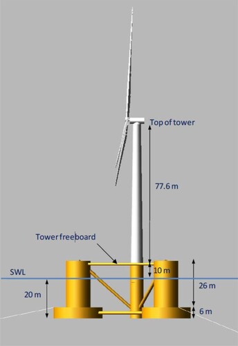
Table 1. Parameters of NREL 5 MW wind turbine.

Parameter	Value
Rating	5 MW
Rotor orientation, configuration	Upwind, 3 blades
Radius of rotor	63 m
Radius of hub	1.5 m
Hub height	90 m
Cut-in, rated, cut-out wind speed	3, 11.4, 25 m/s
Cut-in, rated rotor speed	6.9, 12.1 rpm
Rated tip speed	80 m/s
Blade length	61.5 m
Blade mass	16,450 kg
Rotor mass	110,000 kg
Nacelle mass	240,000 kg
Tower mass	347,460 kg

Table 2. Characteristics of the OC4-DeepCwind semi-submersible platform.

Items	Value
Depth to platform base below SWL (total draft)	20.0 m
Elevation to platform top (tower base) above SWL	10.0 m
Platform mass, including ballast	1.3473E + 7 kg kg
CM location below SWL	13.46 m
Platform roll inertia about CM	6.827E + 9 kg·m^2
Platform pitch inertia about CM	6.827E + 9 kg·m^2
Platform Yaw inertia about platform centreline	1.226E + 10 kg·m^2

Table 3. Mooring system properties.

Items	Value
Number of mooring lines	3
Angle between adjacent lines	120°
Depth to anchors below SWL	200 m
Depth to fairleads below SWL	14 m
Radius to anchors from platform centreline	837.6 m
Radius to fairleads from platform centreline	40.868 m
Unstretched mooring line length	835.5 m
Mooring line diameter	0.0766 m
Equivalent mooring line mass density	113.35 kg/m
Equivalent mooring line mass in water	108.63 kg/m
Equivalent mooring line extensional stiffness	753.6 MN
Pretension of mooring lines	1103.5 kN

2.3. Extreme operating gust (EOG) description

Several types of extreme wind models are specified in the ABS rules (ABS, 2020) and DNV rules (DNV, 2021). One of the conditions, EOG, has been identified to threaten the safety of the wind turbine in previous studies (Zhang et al., 2023). The main feature of the EOG is the sudden increase and then decrease of wind speed, which can represent a type of extreme gust feature that may exist in the typhoon. Therefore, this paper focuses on the effect of EOG on the prediction of ultimate mooring tension. In ABS and DNV rules, the wind speed V is defined as a function of height z and time t as follows. 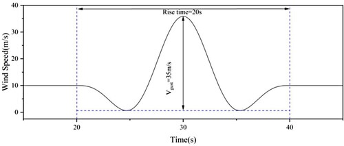(1) $\begin{array}{r}V\left(z,t\right)=\{\begin{array}{ll}V\left(z\right)-0.37V_{\text{gust}}\sin \left(3\pi \mathrm{t}/\text{T}\right)& 0\le t\le T\\ \left[1-\cos \left(3\pi \mathrm{t}/\text{T}\right)\right]& \\ V\left(z\right)& \text{otherwise}\end{array}\end{array}$(1) where V(z) is the wind profile model function, which represents the function of average wind speed with height z, T is the rise time, and V_gust is the amplitude of gust velocity at hub height.

According to the above equation, V(z), V_gust, and T are independent of each other, and these three parameters can determine the characteristics of the EOG condition. Therefore, we can establish the EOG condition in the simulation by confirming the above parameters. For example, assuming V(z) = 10 m/s, V_gust= 35 m/s, and T = 20 s, the derived wind speed profile is shown in Figure 2.

Figure 2. Schematic diagram of EOG wind speed variation.

2.4. ACER method

ACER method is used to calculate the probability of exceedance based on a cascade of conditional approximations. Suppose that at a time interval (0, T), the random process is at the discrete-time t₁, … , t_N. There are N observations in X₁, … , X_N. The goal is to accurately determine the distribution function of extreme value $M_N=\text{max}\left\{X_j;j=1,\cdots ,N\right\}$. The value of $P\left(\eta \right)=\text{Prob}\left(M_N\le \eta \right)$ is the estimation of large values of η.

The definition of P(η) follows (2) $\begin{array}{rl}P\left(\eta \right)& =\text{Prob}\left\{X_1\le \eta ,\cdots ,X_N\le \eta \right\}\\ & =\text{Prob}\left\{X_N\le \eta |X_1\le \eta ,\cdots ,X_{N-1}\le \eta \right\}\\ & \text{Prob}\left\{X_1\le \eta ,\cdots ,X_{N-1}\le \eta \right\}\\ & =\prod _{j=2}^N\text{Prob}\left\{X_j\le \eta |X_1\le \eta ,\cdots ,X_{j-1}\le \eta \right\}\\ & \times P\left(X_1\le \eta \right)\end{array}$(2) By assuming that all X_j are statistically independent, P(η) is approximated as (3) $P\left(\eta \right)\approx \prod _{j=2}^{N}P\left(X_j\le \eta \right)$(3)

The conditional exceeding probability is defined as (4) ${\alpha }_{\mathrm{kj}}=\text{Prob}\left\{X_j>\eta |X_{j-k+1}\le \eta ,\cdots ,X_{j-1}\le \eta \right\}$(4) where α_kj represents the probability of exceeding the standard if the previous k-1 has not exceeded the standard.

Assuming the condition exceedance events are independent and follow the Poisson process, the extreme value distribution can be approximated as (5) $P_k\left(\eta \right)\approx \exp \left(-\sum _{j=k}^N{\alpha }_{\mathrm{kj}}\left(\eta \right)\right)$(5) where $\sum _{j=k}^N{\alpha }_{\mathrm{kj}}\left(\eta \right)$ is the expected effective number of exceedances provided by conditioning on k-1 previous observations.

The average conditional exceedance rate (ACER) is defined as (6) ${\overline{ϵ}}_k=\frac{1}{N-k+1}\sum _{j=k}^N{\alpha }_{\mathrm{kj}}\left(\eta \right)k=1,2,\cdots$(6) For stationary and non-stationary time series, the sample estimate for ACER is (7) ${\widehat{ϵ}}_k\left(\eta \right)=\frac{1}{M}\sum _{m=1}^M{\widehat{ϵ}}_k^{\left(m\right)}\left(\eta \right)$(7) where M is the sample size and exponent (m) refers to the realized quantity M.

Assume the samples are independent, and the 95% confidence interval (CI) for ACER is shown as below. (8) $C{I}^{\pm }\left(\eta \right)={\widehat{ϵ}}_k\left(\eta \right)\pm \frac{1.96\widehat{S_k}\left(\eta \right)}{\sqrt{M}}$(8) where $\widehat{S_k}\left(\eta \right)$ is the standard deviation of ${\widehat{ϵ}}_k\left(\eta \right)$. (9) $\widehat{S_k}{\left(\eta \right)}^2=\frac{1}{M-1}\sum _{m=1}^M{\left({\widehat{ϵ}}_k^{\left(m\right)}\left(\eta \right)-{\widehat{ϵ}}_k\left(\eta \right)\right)}^2$(9)

Use the Gumbel asymptotic form as a guide, and assume that the behaviour of the tail average exceedance rate is determined by $\text{exp}\left\{-a{\left(\eta -b\right)}^c\right\}\left(\eta \ge {\eta }_1\ge b\right)$. Therefore, it can be assumed as follows. (10) ${ϵ}_k\left(\eta \right)\approx q_k\left(\eta \right)\exp \left\{-a_k{\left(\eta -b_k\right)}^{C_k}\right\}\eta \ge {\eta }_1$(10) here a_k, b_k, c_k, and q_k are k-related parameters, and η₁ is the appropriately selected tail marker threshold.

This fitting function achieves the following important goals. First, the parameter class contains the form given by c_k= q_k= 1 as a special case, which corresponds to the Gumbel distribution and is a special case of assumed tail behaviour. Second, this class of functions is flexible enough to capture to some extent the sub-asymptotic behaviour of any extreme value distribution, the asymptotic Gumbel distribution. Third, parametric functions agree with several known exceptions, one of the most important examples being the extreme distribution of a regular static Gaussian process with c_k= 2.

Parameters a, b, c, and q are determined by minimizing the following mean-square error functions with all four independent variables. (11) $\begin{array}{r}F\left(a,b,c,q\right)=\sum _{j=1}^R{\omega }_j{|\log {\widehat{ϵ}}_k\left({\eta }_j\right)-\log q+a{\left({\eta }_j-b\right)}^c|}^2\end{array}$(11) where η₁< … <η_R denotes the level of the estimated ACER function and w_j denotes the weighting factor, with the following equation. (12) ${\omega }_j={\left(\log C^{+}\left({\eta }_j\right)-\log C^{-}\left({\eta }_j\right)\right)}^{-\theta }$(12) where $\theta$ = 1 or 2, usually. According to Naess et al., choosing either one usually works well. Xu et al., (2021) used θ = 2 in their study of mooring tension extremes, and θ = 2 is also used in this study.

By denoting a and q by b and c, the four-parameter optimization problem can be reduced to two parameters (Saha et al., 2014). (13) $\begin{array}{rl}{z}_j& =\log {ϵ}_k\left({\eta }_j\right)\end{array}$(13) (14) $\begin{array}{rl}{y}_j& ={\left({\eta }_j-b\right)}^c\end{array}$(14) (15) $\begin{array}{rl}{a}^{\ast }\left(b,c\right)& =-\frac{\sum _{j=1}^R{\omega }_j\left(y_j-\overline{y}\right)\left(z_j-\overline{z}\right)}{\sum _{j=1}^R{\omega }_j{\left(y_j-\overline{y}\right)}^2}\end{array}$(15) (16) $\begin{array}{rl}\log q^{\ast }\left(b,c\right)& =\overline{z}+a^{\ast }\left(b,c\right)\overline{y}\end{array}$(16) (17) $\begin{array}{rl}\overline{y}& =\frac{\sum _{j=1}^R{\omega }_j{y}_j}{\sum _{j=1}^R{\omega }_j}\end{array}$(17) (18) $\begin{array}{rl}\overline{z}& =\frac{\sum _{j=1}^R{\omega }_j{z}_j}{\sum _{j=1}^R{\omega }_j}\end{array}$(18)

Now, the equation becomes (19) $\begin{array}{r}\tilde{F}\left(b,c\right)=F\left(a^{\ast }\left(b,c\right),b,c,q^{\ast }\left(b,c\right)\right)\end{array}$(19) To improve the robustness of the results, some constraints are applied. (20) $\begin{array}{c}0<c<5\\ min\left(X_j\right)<b<{\eta }_1\\ 0<q<+\mathrm{\infty }\\ 0<a<+\mathrm{\infty }\end{array}$(20)

Apply the Levenberg–Marquardt method to solve Equation (19) and find b and c. Parameters a and q are then calculated by substituting b and c into Equations (15) and (16).

3. Identification of hazardous EOG condition of mooring line

EOG is commonly used to study extreme response problems under turbine operating conditions due to its abrupt variability. However, encountering 100-year severe sea state, FOWT will be in a prepared shutdown state. Considering that extreme gusts of abrupt variable types in typhoons may also significantly affect the mooring tension of FOWT in shutdown conditions, the EOG model is used in this paper to study the effect of gusts with abrupt variable wind speed on the extreme values of mooring tension.

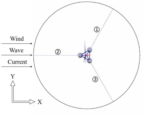
The 100-year survival state described by the JONSWAP spectrum is considered, in which the wave and current conditions are Hs = 10.5 m, Tp = 14.3 s, and V_current= 0.85 m/s. The wave conditions take into account a 100-year extreme sea state tested by Coulling et al. (2013) in the DeepCwind experiment. Extreme current speeds are determined based on annual velocity data in the South China Sea. The wind turbine has been shut down due to the assumption that it is in 100-year typhoon condition. The arrangement of the mooring lines and the incident direction of the wind and wave currents are shown in Figure 3. Since the No. 2 mooring line (Moor_2) is subjected to the maximum mooring tension, the paper chooses the No. 2 mooring line as the object of the study.

Figure 3. Schematic diagram of mooring line arrangement for NREL 5MW wind turbine.

Considering the actual marine environment of the South China Sea, V_gust= 35 m/s is almost an extreme case, in accord with the statistical data, this paper adopts the EOG gust with V_gust= 35 m/s and a rise time of 20 s to study the effect on the mooring line tension extremes.

When the EOG occurs at different moments, the FOWT platform will be in different longitudinal positions. The differences are seen in the peak values of mooring tensions due to the stochastic nature of wind-wave coupling. In this paper, several hazardous cases are screened to show the obvious effects of EOG on mooring tensions. For this FOWT, in the numerical simulation with a period of 2500 s, the typical start times of EOG are randomly selected as 912, 1295, and 2318 s. Otherwise, a case with EOG occurring at a random moment, 1500s, is also studied. The time series of mooring tensions for the FOWT are shown in Figure 4, and the surge motions are shown in Figure 5.

Figure 4. Time-history Moor_2 line tension of FOWT when different EOG occurrences.

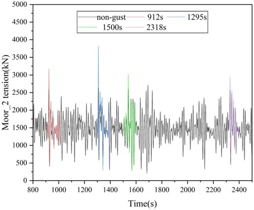
Figure 5. Surge motion of FOWT for different EOG occurrences.

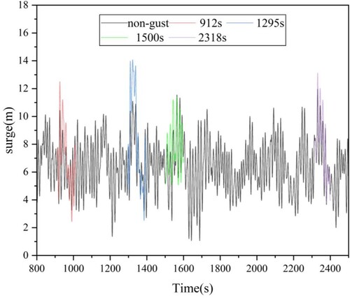
In the case of 1295 s, for example, the platform reached a maximum surge displacement of 11.09 m in the absence of gusts when the front Moor_2 line was in a pronounced state of stretch. Under gust loading, the floating platform generates an additional 2.99 m of surge displacement, reaching the maximum surge of 14.08 m, resulting in a greater mooring line stretch. This results in an increase in mooring tension to 4172 kN, more than 40% of that in non-gust case. The reason is that the platform surge increases and then decreases under non-gust conditions, which leads to a large loose-tightened-loose trend in the mooring line. The presence of EOG exacerbated that trend again, leading to a sharp increase in mooring tension. The values are also increased in other hazardous situations, ranging from 10 to 30%.

The above analysis of the extreme mooring tension of FOWT under the influence of EOG shows that extreme gusts can increase the mooring tension sharply. If extreme gusts are ignored, the extreme tension of mooring lines may be underestimated.

4. Predicting the extreme tensions of mooring lines in a 100-year typhoon

This section will estimate the tension extremes of 3, 12, and 24 h for the mooring lines under stable winds and EOG in 100-year typhoon conditions.

Typhoons generally last for 20–30 h (Wang et al., 2017). To obtain a complete load history during a typhoon period, the German BSH standard (BSH, 2015) proposes a design duration of 35 h. To analyse the extreme values of mooring lines in typhoons, this study focuses on shorter durations, such as 3, 12, and 24 h, to complete short-term predictions. And 24 h can probably cover the period generating the largest mooring tension of the FOWT.

Despite the feasibility of studying the extremes of the mooring tension with a fully coupled dynamic simulation analysis for the whole phase (3, 12, and 24 h), the computational expense will grow rapidly with operating conditions and simulation length (Xu & Guedes Soares, 2023). Therefore, we used the 1-h fully coupled simulation results as a sample. In addition, the uncertainty of wave train is taken into account in extreme value predicting, so we used several samples of 1-h simulation data in ocean conditions with ten different wave seeds to predict the 3-, 12-, and 24-h return values, respectively.

The ACER method was used to predict the extreme tensions of mooring lines. The tension of the mooring line is first evaluated for the average exceedance rate at different values of k. The order of the available k is then determined based on the convergence of the tail data. Then, an asymptotic Gumbel-type fitting function is used to fit the tail data of the average exceedance rate in the determined order of the available k. Finally, the corresponding extreme value can be obtained based on the return probability corresponding to the requested return period.

4.1. Effect of extreme gusts on the ultimate mooring tension prediction

The 100-year sea state described in section 3 was combined with three different wind conditions, as shown in Table 4. The wind speed is stable at 10 m/s in Case 1, and EOG occurs in Cases 2 and 3, with the parameters V(z) = 10 m/s, V_gust= 35 m/s, and T = 20s. And the wind speeds are stable at 10 m/s for the rest of the time in Cases 2 and 3. In Case 2, the EOG appears at 1500 s representing a random moment. Case 3 chooses the most hazardous condition with a specific EOG starting moment among the studied cases in section 3.

Table 4. Environmental parameters under 100-year typhoon

Case	Wind of EOG	Wave	Current (Uniform flow)
Case 1	Stationary wind Vwind = 10 m/s	JONSWAP spectrum, significant wave height, Hs = 10.5 m; peak spectral period, Tp  = 14.3s.	Uniform flow, water surface current speed, V = 0.85 m/s.
Case 2	V(z) = 10 m/s Vgust = 35 m/s T = 20s EOG start time-a random moment:1500 s
Case 3	V(z) = 10 m/s Vgust = 35 m/s T = 20s EOG start time: Identified hazardous condition

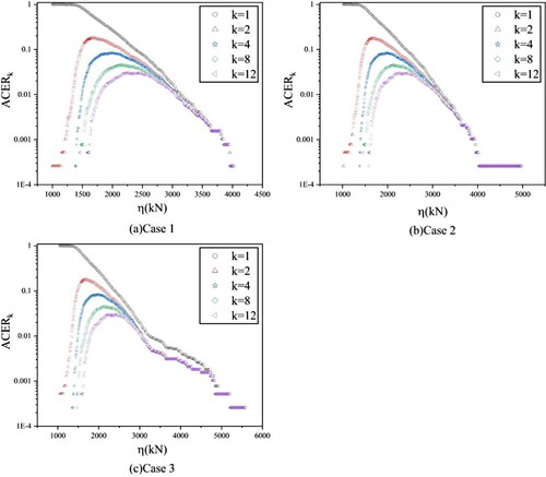
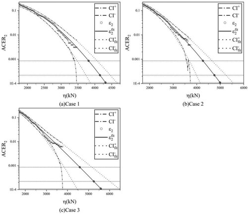
The ACER method is used to predict the short-term mooring tension extremes for the three cases. The unstable simulation results for the first 300s of each sample are ignored and the remaining data is used for ACER analysis. The key to accurately predicting the extreme value by the ACER method lies in fitting the tail data. The convergence of the tail of the ACER function means relatively accurate predicted values can be obtained. To determine the number of orders available for k and to reduce the computational effort, we choose the cases k = 1, 2, 4, 8, and 12 to observe the convergence of the tails of the conditional exceedance probability. The obtained conditional exceedance probabilities are shown in Figure 6. When k > 1, all the ACER functions of order k converge in the tails almost in the same trend and are almost indistinguishable in the tails. Therefore, no substantial difference in the ACER function exists between different values of k. The parameter k has little impact on the difference in ACER values. Among the k-order convergent ACER functions, the one with the fewer orders should be chosen, which contains more complete information about the data and gives more accurate results. The ACER function with k = 2 is chosen to investigate the mooring tension extremes of the wind turbine platform and is denoted as ACER₂.

Figure 6. k-order ACER plots of mooring tension for Cases 1, 2, and 3.

The results of extrapolating the ACER₂ function for 3, 12, and 24 h return periods for the three cases are shown in Figure 7. The solid line (${ϵ}_2^{\mathrm{fit}}$) represents the extrapolated curve fitted to the average exceedance rate (${ϵ}_2$). The intersections of the solid line with the three horizontal dotted lines indicate the return values for 3, 12, and 24 h, respectively. The dotted line ($C{I}_{\mathrm{fit}}^{\pm }$) indicates the 95% CI of the fitted extrapolation curve. The dotted line ($C{I}^{\pm }$) represents the 95% CI obtained directly from the estimation for the average exceedance rate.

Figure 7. Predictions of mooring tension extremes for Cases 1, 2 and 3.

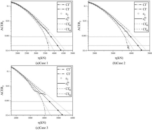
Based on the tail features of ACER₂ in Figure 7, the tail features in Case 1 and Case 2 are seen relatively similar, and the gusts that appear at 1500 s in the Case 2 sample will not significantly affect the emergence of the mooring tension extremes. The reason is the random occurrence of extreme gusts coupled with waves does not necessarily lead to extreme tensions. Random extreme gusts have a limited effect on extreme tensions. The ACER₂ function tails of the Case 3 samples show significant discrete line segments. The coupling of the occurrence of extreme gusts with hazardous conditions results in a dramatic increase in the mooring tension, which greatly increases the extreme values of the mooring tension over the simulation time. However, extreme mooring tensions occur less frequently. Discrete line segments appear on the tail of the ACER curve when the critical value varies between two neighbouring larger values. The more discrete discontinuous line segments in the tails result in a different trend in the ACER function for the data in the tails than for the data a little earlier. The extrapolated trend of the data where a snap event such as an extreme gust occurs is not the same as the data where no snap event occurs. This may affect the accuracy of the prediction results.

The return values of the specific predictions and the corresponding 95% CI are shown in Table 5. The 3-, 12-, and 24-h predictions obtained in Case 2 sample are higher than those in Case 1, by 3.63%, 4.28%, and 4.57%, respectively. Although the difference in values is not significant, the gap between the two gradually increases as the prediction time increases. Due to the stochastic nature of the coupling of EOG to waves that occur in Case 2. When extreme gusts are coupled with small waves, extreme mooring tensions cannot be generated. The 3-, 12-, and 24-h predicted values in Case 3 are 14.32%, 18.76%, and 20.88% higher than Case 1. It shows when extreme gusts act in coupling with relatively large waves, a sharp increase will appear in the mooring tension. The coupling of extreme gusts with hazardous waves will result in more extreme mooring tensions than in the short term when longer return periods are considered.

Table 5. Specific predictions and 95% CI for mooring tension extremes in Cases 1, 2, and 3.

	3-h		12-h		24-h
Case	Predicted value	CI	Predicted value	CI	Predicted value	CI
Case 1	3824.1	(3557.433, 3989.7)	4178.32	(3828.11, 4378.02)	4349.08	(3955.89, 4565.89)
Case 2	3963.02	(3673.34, 4139.4)	4357.05	(3975.07, 4569.54)	4547.84	(4118.18, 4778.47)
Magnitude of change	+3.63%		4.28%		4.57%
Case 3	4371.57	(3885.04, 4765.62)	4962.21	(4245.09, 5489.14)	5257.2	(4413.38, 5854.43)
Magnitude of change	14.32%		18.76%		20.88%

4.2. Results among different stable wind speeds and extreme gusts

To further show the effect of the occurrence of EOG on the prediction of mooring tension extremes, the results of additional stable winds with different wind speeds and EOG under hazardous conditions are discussed.

The stable 10 m/s wind speed in Case 1 is modified to stable 20 and 30 m/s, denoted as Case 4 and Case 5, respectively. In addition, to verify that extreme gusts under higher stable wind conditions can lead to the same condition as Case 3, the case of extreme gusts at a stable wind speed of 30 m/s is considered, denoted as Case 6. The base wind speed for Case 6 is a stable 30 m/s and the gust parameters are V(z) = 30 m/s, V_gust= 25 m/s, and T = 20s, at which point V_max= 45 m/s occurs at the time of the hazardous conditions identified in the previous section. The reason for choosing this gust parameter is that the maximum wind speed of 45 m/s is close to the maximum wind speed in certain typhoon statistics such as Lekima (52 m/s) (Chi et al., 2022). The specific environmental parameters are shown in Table 6. Figure 8 gives the tension diagrams for Case 4, 5, and 6 when extreme gusts occur under a certain random wave.

Figure 8. Mooring tensions in Cases 4, 5, and 6.

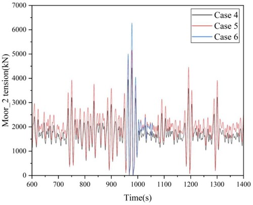
Table 6. Environmental parameters at different wind speeds.

Case	Wind of EOG	Wave	Current (Uniform flow)
Case 4	Stationary wind Vwind = 20 m/s	JONSWAP spectrum, significant wave height, Hs = 10.5 m; peak spectral period, Tp  = 14.3s.	Uniform flow, water surface current speed, V = 0.85 m/s.
Case 5	Stationary wind Vwind = 30 m/s
Case 6	V(z) = 30 m/s Vgust = 20 m/s T = 20s EOG start time: Identified hazardous conditions

The same method is used to predict the mooring tensions for 3, 12, and 24 h under the abovementioned three conditions, and the obtained results are compared with Case 3. The k-order ACER plots for the Case 4, 5, and 6 samples are shown in Figure 9, and the predictions obtained by choosing the ACER function with k = 2 are shown in Figure 10, with the specific predicted values and CI shown in Table 7.

Figure 9. k-order ACER plots of mooring tension for Cases 4, 5, and 6.

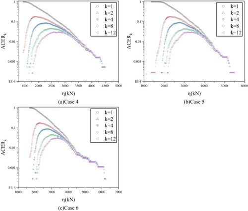
Figure 10. Predictions of mooring tension extremes for Case 4, 5 and 6.

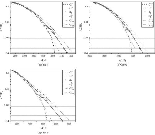
Table 7. Specific predictions and 95% CI for mooring tension extremes for Cases 1, 3, 4, 5, and 6.

	3 h		12 h		24 h
Case	Estimation (kN)	CI (kN)	Estimation (kN)	CI (kN)	Estimation (kN)	CI (kN)
Case 1 (10 m/s)	3824.1	(3557.33, 3989.70)	4178.32	(3828.11, 4378.02)	4349.08	(3955.89, 4565.89)
Case 3 (10–35 m/s)	4371.57	(3885.04, 4765.62)	4962.21	(4245.09, 5489.14)	5257.2	(4413.38, 5854.43)
Case 4 (20 m/s)	4274.77	(3994.12, 4483.02)	4629.64	(4268.53, 4892.66)	4781.24	(4383.68, 5069.47)
Case 5 (30 m/s)	5083.65	(4786.11, 5331.47)	5478.43	(5102.86, 5793.93)	5646.28	(5235.64, 5993.03)
Case 6 (30–45 m/s)	5573.73	(5054.81, 5945.09)	6185.22	(5461.87, 6659.69)	6486.07	(5654.51, 7013.71)

As shown in Table 7, the tension predictions in Case 3 fall between the results for stable wind speeds of 20 and 30 m/s. However, as the prediction period is extended, the prediction value in Case 3 gradually approaches Case 5. When we predict the 3-h return value, the result of Case 3 is 4371.6 kN, which is slightly higher than 4274.8 kN of Case 4 and 5083.65 kN of Case 5. This means that the maximum mooring tension due to the occurrence of EOG for hazardous conditions is roughly comparable to the extreme value of a stable 20 m/s wind speed over a 3-h period under the present environmental conditions. However, the trend in mooring tension predictions in Case 3 appears to be more pronounced than that in Cases 4 and 5. The gap between the predicted values in Case 3 and Case 4 gradually rises as the prediction period rises, and the gap in Case 5 gradually becomes smaller. When we predict 12-h return value the difference between Case 3 and Case 4,5 is +7.19%, −9.42% respectively. In terms of 24-h return value, the gap between Case 3 and Case 4, 5 is +9.96%, −7.40% respectively. As the prediction period increases, the results of Case 3 may exceed Case 5.

For prediction comparison between Case 5 and Case 6 with the original wind speed of 30 m/s. The 3, 12, and 24-h predicted values obtained in the Case 6 sample are 9.64%, 12.91%, and 14.88% higher than Case 5. It can be seen that even for higher-base wind speed, extreme gusts can still significantly affect the prediction of the extreme tension of mooring line.

The extended return period means that extreme gusts are likely to be coupled with more dangerous waves, leading to an increase in extreme mooring tension. This trend is also consistent with the previous judgment on the effect of EOG on mooring tension. The sudden and sharp increase of the mooring tension is characterized by the ‘rightward’ change of the extrapolation trend in the prediction results. To show the difference in this trend more intuitively, the ACER₂ functions and the corresponding fitted curves for Cases 1, 3, 4, and 5 are shown in the same Figure 11. CI and other information are not given.

Figure 11. Extrapolated trends and predictions of mooring tension extremes for Case 1, 3, 4, 5, 6.

Figure 11 shows that the wind speeds in Cases 1, 4, and 5 are stable at 10, 20, and 30 m/s, respectively, and the trends of the data in their tails are all roughly the same. In Case 3, the identified hazardous condition with EOG, the trend of the data at the front end of the ACER function is the same as that of Case 1. However, for the tail data, due to the emergence of extreme mooring tension, the tail appears to be more discrete. The extrapolated trend of the tail data in Case 3 deviates from Case 1. The data almost overlaps at the front end of Cases 6 and 5, and the extrapolated trends in the tails deviate. Case 3 and Case 6 are both affected by extreme gusts, and their extrapolated trends are essentially the same. This suggests that extreme mooring tensions due to EOG make the trend in the tail data inconsistent with the change in the wake trend under stable wind conditions, with a much faster rate of change than under stable winds. When extreme predictions are made for longer return periods, the predicted extreme results increase rapidly.

Building upon the earlier discussion regarding the impact of EOG on mooring tension, it is imperative to acknowledge the influence of EOG on extreme mooring tension even when the turbine is inactive and encountering extreme sea states. Ignoring the effects of EOG would underestimate the extreme design state of mooring lines.

5. Effects of simulation length and sample number on prediction results

Given the above study, it is necessary to investigate the effect of uncertainty in simulation length and sample size on the prediction results, considering that it is possible that different simulation lengths and sample sizes may not affect the prediction results of stable wind speeds and extreme operating gust samples, respectively, to the same extent.

5.1. Effect of simulation duration uncertainty

Due to the uncertainty of the occurrence of such unexpected events as extreme gusts, it is necessary to explore the effect of the simulation duration on the prediction results, considering that the extreme values triggered by extreme gusts may be diluted by the excessively long simulation time.

The simulation duration of the samples was adjusted to investigate the effect of simulation duration on the prediction results. In this part of the study, samples with three different duration simulation times (20 min, 30 min, and 1 h) will be analysed, with each different time sample containing 10 simulations. The first 300 s of unstable data were removed for all three samples. EOG appeared in the 900ths for the 20 and 30 min samples, and extreme gusts still appeared in the 1500s for the 1 h sample.

The k-order ACER plots for the 30 min and 20 min samples are shown in Figures 12 and 13. It shows when k > 1, the ACER₂ function has converged in the tail, which is consistent with the choice of 1 h samples, and the ACER function with k = 2 is chosen for prediction, and the results obtained are shown in Figures 14 and 15.

Figure 12. k-order ACER plot of mooring tension for simulation time of 30 min.

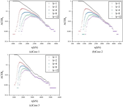
Figure 13. k-order ACER plot of mooring tension for simulation time of 20 min.

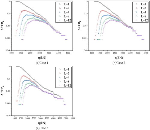
Figure 14. Prediction of mooring tension extremes for samples with simulation time of 30 min.

Figure 15. Prediction of mooring tension extremes for samples with simulation time of 20 min.

To more visually represent the predicted results of tension, the results of using the ACER method for the 3 h return values of extreme mooring tensions for the three scenarios and the 95% confidence intervals are given in Table 8.

Table 8. Specific predictions and 95% CI for mooring tensions for Case 1, 2 and 3 at different durations (1 h, 30, 20 min).

		3-h		12-h		24-h
Case	Simulation time	Predicted value (kN)	CI	Predicted value (kN)	CI	Predicted value (kN)	CI
Case 1	1 h	3824.1	(3557.433, 3989.7)	4178.32	(3828.11, 4378.02)	4349.08	(3955.89, 4565.89)
	30 min	3763.72	(3476.79, 3994.96)	4136.59	(3730.07, 4374.89)	4290.62	(3849.28, 4558.26)
	Magnitude of change	−1.58%		−1.00%		−1.34%
	20 min	3813.57	(3475.52, 4065.98)	4152.47	(3735.98, 4457.39)	4314.48	(3858.73, 4646.03)
	Magnitude of change	+0.28%		+0.62%		+0.80%
Case 2	1 h	3963.02	(3673.34, 4139.4)	4357.05	(3975.07, 4569.54)	4547.84	(4118.18, 4778.47)
	30 min	4067.83	(3634.89, 4332.2)	4488.11	(3922.61, 4808.73)	4691.99	(4058.54, 5041.02)
	Magnitude of change	+2.64%		+3.00%		+3.17%
	20 min	4265.8	(3685.43, 4654.63)	4753.61	(3992.08, 5243.06)	4992.15	(4137.35, 5533.75)
	Magnitude of change	+7.64%		+9.1%		+9.77%
Case 3	1 h	4371.57	(3885.04, 4765.62)	4962.21	(4245.09, 5489.14)	5257.2	(4413.38, 5854.43)
	30 min	4423.21	(3830.89, 4873.33)	5019.86	(4222.83, 5611.25)	5316.88	(4412.62, 5982.85)
	Magnitude of change	+1.18%		+1.16%		+1.14%
	20 min	4586.39	(3844.88, 5163.98)	5248.8	(4250.85, 6009.21)	5580.56	(4447.83, 6438.12)
	Magnitude of change	+4.91%		+5.76%		+6.15%

For the stable wind conditions in Case 1, there is little effect on the prediction results by changing the simulation time. The 3 h return values predicted with 20 min, 30 min, and 1 h simulation timescales are very similar. The difference between the 3, 12, and 24 h return values of tension for the 30 min sample and the 1 h sample were 1.58%, 1.00%, and 1.34%, respectively. The difference between the 20 min sample and the 1 h sample was 0.28%, 0.62%, and 0.80%. The fluctuation among the three predicted values is not large, which shows that the extreme values used for calculation are not sensitive to the duration. In wind turbine research, it has been suggested that a 10-minute duration is used to estimate the 1-hour extreme value (Dimitrov, 2016), which is laterally verified by the results in this paper.

However, if a large or severe contingency occurs within the sample duration, as in the case of EOG studied in this paper, the effect of the sample duration on the prediction results seems to be non-negligible. For Case 2, where extreme gusts occur at a fixed time, and for Case 3, where gusts are coupled with dangerous waves, it is shown that the results of the extreme predictions are then closely related to simulation duration. It can be seen that the 3, 12, and 24-h return values of the predicted mooring tensions become larger and larger as the simulation duration is shortened. For Case 2, the 3, 12, and 24 h returns of tension for the 30 min sample were 2.64%, 3.00%, and 3.17% higher than the 1 h sample, respectively. The 20 min samples were 7.64%, 9.10%, and 9.77% higher than the 1 h samples. For Case 3, the 3, 12, and 24 h return values of tension for the 30 min sample were 1.18%, 1.16%, and 1.14% higher than the 1 h sample, respectively. The 20 min samples were 4.91%, 5.76%, and 6.15% higher than the 1 h samples.

To discuss the effect of sample duration on the prediction results, it is firstly clarified that the extreme gusts in this paper are set to occur only once at a certain time in the simulation. For the prediction of a certain period, the shortening of the simulation time represents an increase in the frequency of the occurrence of extreme gusts. For example, if the same return value is predicted for 3 h, a simulation time of 20 min indicates that extreme gusts will occur more frequently than for 1 h. The frequency of the occurrence of extreme gusts increases, and the predicted values of mooring tensions obtained increase as a result. Therefore, to obtain more accurate predictions, more detailed statistics are needed to determine how frequently extreme gusts occur.

5.2. Effect of sample size uncertainty

Since extreme gusts are highly contingent contingencies and the effect of extreme gusts coupled with different waves on the tension in the mooring system of the wind turbine platform cannot be accurately determined, it is necessary to explore the effect of sample size on the prediction results to ensure the accuracy of the prediction results.

The number of samples was adjusted to investigate the effect of sample size on the prediction results. In the previous section of the study, the number of simulations for each of the three scenarios was determined to be 10. In this part of the study, predictions will be made for samples containing different numbers of simulations by randomly selecting between three and seven simulations out of the ten simulations (simulation numbers 3, 5, and 7, respectively). For all three samples, the first 300s of unstable data were removed. 20 and 30 min samples had extreme gusts occurring in the 900s, and the 1 h sample still had extreme gusts occurring in the 1500s.

To express the prediction results concisely and clearly, this part only discusses the prediction values of mooring tension 3 h. The picture only gives the ACER₂ function, the fitted curves, and the prediction results, and the confidence interval of the prediction results is no longer given.

The prediction results obtained for Cases 1, 2, and 3 with different simulation durations and different sample sizes are shown in Figures 16–18. The red dots and solid lines in the figures indicate the ACER₂ function and the corresponding fitted curves for 3 simulations, respectively. The black dots and the underlined lines indicate the ACER₂ function for 5 simulations of the data and the corresponding fitted curves. The blue dots and dotted lines indicate the ACER₂ function for the seven simulations and the corresponding fitted curves, respectively. The specific predicted values are shown in Table 9. For better comparison, the predictions of the 10 simulations obtained in the previous section are added to the table for comparison.

Figure 16. Prediction of mooring tension extremes of (sample sizes 3, 5, 7), Case 1 with different sample sizes.

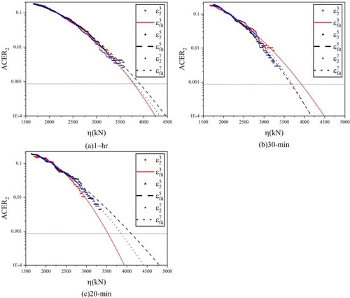
Figure 17. Prediction of mooring tension extremes of (sample sizes 3, 5, 7), Case 2 with different sample sizes.

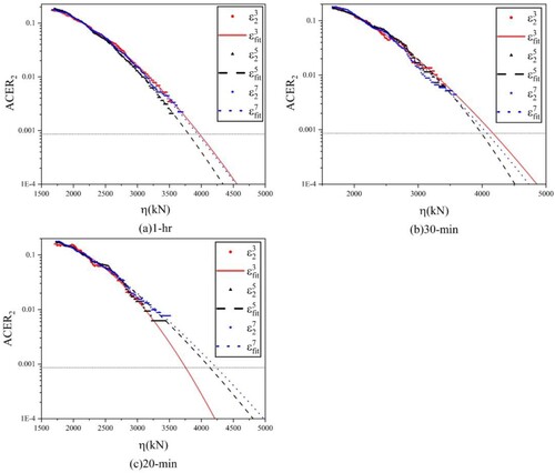
Figure 18. Prediction of mooring tension extremes of (sample sizes 3, 5, 7), Case 3 with different sample sizes.

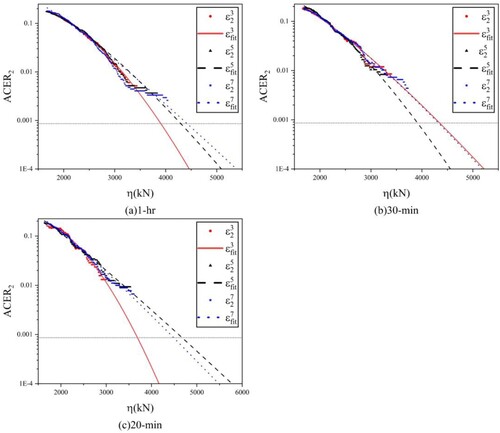
Table 9. Specific predictions of mooring tensions for different sample sizes (3, 5, 7, 10), Case 1, 2, 3.

		Sample size
Case	Simulation time	3	5	7	10
Case 1	1 h	3787.69	3916.58	3806.47	3824.1
	30 min	3924.35	3669.41	3701.1	3763.72
	20 min	3532.89	4106.42	3857.16	3813.57
Case 2	1 h	3973.12	3801.79	3941.4	3963.02
	30 min	4170.97	3989.89	4076.36	4067.83
	20 min	3755.57	4135.43	4237.17	4265.8
Case 3	1 h	3904.31	4295.61	4419.45	4371.57
	30 min	4347.81	3914.13	4340.84	4423.21
	20 min	3688.5	4674.37	4487.41	4586.39

In Figures 16–18, ${ϵ}_2^3$, ${ϵ}_2^5$, ${ϵ}_2^7$ denote the average exceedance of mooring tensions for k = 2 with sample sizes of 3, 5, and 7, respectively, and ${ϵ}_{\mathrm{fit}}^3$, ${ϵ}_{\mathrm{fit}}^5$, ${ϵ}_{\mathrm{fit}}^7$ denote the fitted curves for k = 2 with sample sizes of 3, 5, and 7, respectively. The intersection of the fitted curve with the dotted line is then the predicted value for 3 h.

Based on the results in Figures 16–18 and Table 9, it can be seen that when the number of samples is small, the results obtained from the prediction fluctuate greatly. When the number of samples is small, such as the occurrence of a single very extreme mooring tension, it may lead to excessive bias in the prediction results. For Case 1 where no extreme gusts occur, the occurrence of extreme mooring tension is largely dependent on waves. The predictions are fluctuating but within acceptable limits. However, for Case 2 and Case 3, the occurrence of EOG exacerbates the emergence of extreme mooring tension as well as chance. When the number of samples is too small, the trends may show inconsistent predicted trends with sufficient samples, which may lead to excessive bias in the prediction results. For example, in Case 3, the prediction result for a simulation time of 20 min and sample size of 3 is 3688.5kN. However, the prediction result for a simulation time of 20 min and sample size of 10 is 4586.39kN, which is a difference of 24.34%.

Therefore, to ensure the accuracy of the prediction results, it is necessary to ensure that there is a sufficient number of samples. When the number of samples is 7 and 10, the tail marks of the 7-sample data set converge to the 10-sample data set, and the tail trends of both are the same, and the prediction results obtained are almost the same. 10–20 samples are also recommended in the DNV specification (DNV, 2021) for the prediction of extreme values. The DNV specification also recommends the use of 10–20 samples for the prediction of extreme values. It shows that 10 samples can provide sufficient data for the prediction of mooring tension.

With the effects of simulation length and sample size on the prediction results discussed above, the simulation time as well as the sample size have a limited effect on the prediction results when EOG does not occur. For the simulation time, the 20-min simulation length is sufficient to predict the 3-h return value by applying the ACER method for extreme prediction. However, for cases where EOG occurs, the simulation time is too short and the number of samples is too small to represent the true distribution of the mooring tension. This may lead to excessive deviations of the predicted results from the actual values. Therefore, it is necessary to appropriately extend the length of the simulation or increase the number of samples, which can lead to more accurate prediction results. The conclusion may apply to other snap events.

6. Conclusion

Currently, the commonly used approach for general ultimate state design is the Extreme Typhoon Model (ETM). However, this paper considers the inclusion of EOG in extreme ocean environments to assess the extreme mooring tension of an FOWT and estimate the effect on the limit design state of the mooring system.

The paper commences with an examination of the effect of EOG on the mooring tension. The most significant impact occurs when the upward cycle of the EOG aligns with the platform's relaxation-tightness-relaxation trend. Subsequently, the paper predicts the mooring tension under extreme gust conditions during 100-year sea state, and investigates the influence of EOG on the prediction results. It also discusses the impact of simulation duration and sample size on the prediction results in the presence of EOG. The primary conclusions of this study are as follows:

1. When the motion of FOWT exhibits a significant relaxation-tightening-relaxation trend, a coupled EOG will result in extreme mooring tension. In the case studied in this paper, the maximum mooring tension can exceed 40% compared with that in non-gust cases in the most severe scenarios.

2. Extreme mooring tensions cause the data in the tail of the mooring tension ACER function to exhibit discrete line segments, with the extrapolated trend deviating from the non-gust trend. This feature leads to a rapid increase in predicted values with an increasing return period, corresponding to a large transient change in wind loads that sharply elevates mooring tension.

3. For environmental conditions where extreme emergencies rarely occur, a simulation time of 20 min can be employed to predict the 3-h extreme values. However, when predicting snap events, using a short sample or small sample size can introduce errors in the results. Detailed statistical analysis of emergency frequencies is essential for obtaining accurate predictions.

4. For the Ultimate Limit State (ULS) design of FOWT mooring system, snap events such as EOG should be considered. In this paper, the predictions of mooring tension of FOWT under gust conditions are 14–20% larger than that under stable wind conditions. Failure to consider contingencies such as EOG will lead to a underestimation of extreme mooring tensions.

The paper demonstrates that certain abrupt loads can trigger a sudden and drastic increase in mooring line tension. Ignoring extreme wind conditions during typhoons may lead to an underestimation of the mooring tension extremes. The findings of this study can serve as a reference for the limit state design of floating wind turbine mooring systems.

This paper specifically focuses on predicting tension extremes for a single type of EOG under 100-year typhoon conditions and does not explore the effects of other extreme wind models. Therefore, future research should investigate additional influencing factors and extreme wind conditions in the context of the actual marine environment to better understand the environmental conditions that threaten mooring system safety and accurately predict extreme mooring line tension.

Disclosure statement

No potential conflict of interest was reported by the author(s).

Additional information

Funding

This work is supported by the National Natural Science Foundation of China (Grant No. 52301356), the National Key Research and Development Program of China (Grant No. 2022YFC2806300), and the Innovation Group Project of Southern· Marine· Science and Engineering· Guangdong (No. SML2022016).

References

- American Bureau of Shipping. (2020). ABS guide for building and classing-floating offshore wind turbine.
- Brommundt, M., Krause, L. C., Merz, K. O., & Muskulus, M. (2012). Mooring system optimization for floating wind turbines using frequency domain analysis. Energy Procedia, 24, 289–296. https://doi.org/10.1016/j.egypro.2012.06.111
- Bundesamt für Seeschifffahrt und Hydrographie. (2015). Standard design: Minimum requirements concerning the constructive design of offshore structures with the Exclusive Economic Zone (EEZ), 1st update.
- Cao, S., Tamura, Y., Kikuchi, N., Saito, M., Nakayama, I., & Yutaka, M. (2015). A case study of gust factor of a strong typhoon. Journal of Wind Engineering and Industrial Aerodynamics, 138, 52–60. https://doi.org/10.1016/j.jweia.2014.12.012
- Chen, M., Jiang, J., Zhang, W., Li, C. B., Zhou, H., Jiang, Y., & Sun, X. (2023a). Study on mooring design of 15 MW floating wind turbines in South China Sea. Journal of Marine Science and Engineering, 12(1), 33. https://doi.org/10.3390/jmse12010033
- Chen, M., Li, C. X., Han, Z., & Lee, J. (2023b). A simulation technique for monitoring the real-time stress responses of various mooring configurations for offshore floating wind turbines. Ocean Engineering, 278, 114366. https://doi.org/10.1016/j.oceaneng.2023.114366
- Chi, W., Shu, F., Lin, Y., Li, Y. F., Luo, F., He, J., Chen, Z., Zou, X., & Zheng, B. (2022). Typhoon-induced destruction and reconstruction of the coastal current system on the inner shelf of East China Sea. Continental Shelf Research, 255, 104912. https://doi.org/10.1016/j.csr.2022.104912
- Coulling, A. J., Goupee, A. J., Robertson, A. N., Jonkman, J. M., & Dagher, H. J. (2013). Validation of a FAST semi-submersible floating wind turbine numerical model with DeepCwind test data. Journal of Renewable and Sustainable Energy, 5(2), 557–569. https://doi.org/10.1063/1.4796197.
- Dimitrov, N. (2016). Comparative analysis of methods for modelling the short-term probability distribution of extreme wind turbine loads. Wind Energy, 19(4), 717–737. https://doi.org/10.1002/we.1861
- Ding, J., Gong, K., & Chen, X. (2013). Comparison of statistical extrapolation methods for the evaluation of long-term extreme response of wind turbine. Engineering Structures, 57, 100–115. https://doi.org/10.1016/j.engstruct.2013.09.017
- DNV. (2021). Floating wind turbine structures. Offshore standard DNV-ST-0119.
- Fogle, J., Agarwal, P., & Manuel, L. (2008). Towards an improved understanding of statistical extrapolation for wind turbine extreme loads. Wind Energy, 11(6), 613–635. https://doi.org/10.1002/we.303
- Freudenreich, K., & Argyriadis, K. (2008). Wind turbine load level based on extrapolation and simplified methods. Wind Energy, 11(6), 589–600. https://doi.org/10.1002/we.279
- Fu, P., Leira, B. J., Myrhaug, D., & Chai, W. (2021). Assessment of methods for short-term analysis of riser collision probability. Ocean Engineering, 238, 109221. https://doi.org/10.1016/j.oceaneng.2021.109221
- Gong, K., Ding, J., & Chen, X. (2014). Estimation of long-term extreme response of operational and parked wind turbines: Validation and some new insights. Engineering Structures, 81, 135–147. https://doi.org/10.1016/j.engstruct.2014.09.039
- Hou, H., & Liu, Y. J. (2023). Analysis of the upper tail of the short-term extreme tension distribution of mooring line by the peaks-over-threshold method. Ocean Engineering, 281, 114994. https://doi.org/10.1016/j.oceaneng.2023.114994
- Hsu, W., Thiagarajan, K. P., MacNicoll, M., & Akers, R. (2015). Prediction of extreme tensions in mooring lines of a floating offshore wind turbine in a 100-year storm.
- Jonathan, P., & Ewans, K. C. (2013). Statistical modelling of extreme ocean environments for marine design: A review. Ocean Engineering, 62, 91–109. https://doi.org/10.1016/j.oceaneng.2013.01.004
- Jonkman, J. M., Butterfield, S., Musial, W., & Scott, G. N. (2009). Definition of a 5-MW reference wind turbine for offshore system development.
- Liu, S., Chuang, Z., Qu, Y., Li, X., Li, C., & He, Z. (2022). Dynamic performance evaluation of an integrated 15 MW floating offshore wind turbine under typhoon and ECD conditions. Frontiers in Energy Research, 10, 874438. https://doi.org/10.3389/fenrg.2022.874438
- Ma, G., Zhong, L., Zhang, X., Ma, Q., & Kang, H. S. (2020). Mechanism of mooring line breakage of floating offshore wind turbine under extreme coherent gust with direction change condition. Journal of Marine Science and Technology, 25, 1–13. https://doi.org/10.1007/s00773-020-00714-9
- Moan, T., Gao, Z., Bachynski, E. E., & Nejad, A. R. (2020). Recent advances in integrated response analysis of floating wind turbines in a reliability perspective. Journal of Offshore Mechanics and Arctic Engineering-transactions of The Asme, 142(5), 052002. https://doi.org/10.1115/1.4046196
- Moriarty, P., Holley, W., & Butterfield, S. (2002). Effect of turbulence variation on extreme loads prediction for wind turbines. Journal of Solar Energy Engineering-transactions of The Asme, 124(4), 387–395. https://doi.org/10.1115/1.1510137
- Naess, A., & Gaidai, O. (2009). Estimation of extreme values from sampled time series. Structural Safety, 31(4), 325–334. https://doi.org/10.1016/j.strusafe.2008.06.021
- Pickands, J. (1975). Statistical inference using extreme order statistics. Annals of Statistics, 3(1), 119–131.
- Ragan, P., & Manuel, L. (2007). Statistical extrapolation methods for estimating wind turbine extreme loads. Journal of Solar Energy Engineering-transactions of the Asme, 130(3), 031011. https://doi.org/10.1115/1.2931501
- Ren, Y., Shi, W., Venugopal, V., Zhang, L., & Li, X. (2024). Experimental study of tendon failure analysis for a TLP floating offshore wind turbine. Applied Energy, 358, 122633. https://doi.org/10.1016/j.apenergy.2024.122633
- Robertson, A. N., Jonkman, J. M., Masciola, M., Song, H. W., Goupee, A. J., Coulling, A. J., & Luan, C. (2014). Definition of the semisubmersible floating system for phase II of OC4.
- Saha, N., Gao, Z., Moan, T., & Naess, A. (2014). Short-term extreme response analysis of a jacket supporting an offshore wind turbine. Wind Energy, 17(1), 87–104. https://doi.org/10.1002/we.1561
- Silva-González, F. L., Heredia-Zavoni, E., & Inda-Sarmiento, G. (2017). Square error method for threshold estimation in extreme value analysis of wave heights. Ocean Engineering, 137, 138–150. https://doi.org/10.1016/j.oceaneng.2017.03.028
- Sinsabvarodom, C., Leira, B. J., Chai, W., & Næss, A. (2021). Short-term extreme mooring loads prediction and fatigue damage evaluation for station-keeping trials in ice. Ocean Engineering, 242, 109930. https://doi.org/10.1016/j.oceaneng.2021.109930
- Stanisic, D., Efthymiou, M., Kimiaei, M., & Zhao, W. (2018). Design loads and long term distribution of mooring line response of a large weathervaning vessel in a tropical cyclone environment. Marine Structures, 61, 361–380. https://doi.org/10.1016/j.marstruc.2018.06.004
- Wang, X., Huang, P., Yu, X., Wang, X., & Liu, H. (2017). Wind characteristics near the ground during typhoon Meari. Journal of Zhejiang University-SCIENCE A, 18(1), 33–48. https://doi.org/10.1631/jzus.A1500310
- Wang, Y. (2017). Optimal threshold selection in the POT method for extreme value prediction of the dynamic responses of a spar-type floating wind turbine. Ocean Engineering, 134, 119–128. https://doi.org/10.1016/j.oceaneng.2017.02.029
- Xu, S., & Guedes Soares, C. (2023). Parametric study on the short-term extreme mooring tension of nylon rope for a point absorber. Ocean Engineering, 267, 113248. https://doi.org/10.1016/j.oceaneng.2022.113248
- Xu, S., Ji, C., & Soares, C. (2021). Short-term extreme mooring tension and uncertainty analysis by a modified ACER method with adaptive Markov chain Monte Carlo simulations. Ocean Engineering, 236, 109445. https://doi.org/10.1016/j.oceaneng.2021.109445
- Xu, X., Wang, F., Gaidai, O., Naess, A., Xing, Y., & Wang, J. (2022). Bivariate statistics of floating offshore wind turbine dynamic response under operational conditions. Ocean Engineering, 257, 111657. https://doi.org/10.1016/j.oceaneng.2022.111657
- Yang, Q., Li, Y., Li, T., Zhou, X., Huang, G., & Lian, J. (2022). Statistical extrapolation methods and empirical formulae for estimating extreme loads on operating wind turbine towers. Engineering Structures, 267, 114667. https://doi.org/10.1016/j.engstruct.2022.114667
- Yu, S., Wu, W., Bin, X., Wang, S., & Naess, A. (2020). Extreme value prediction of current profiles in the South China Sea based on EOFs and the ACER method. Applied Ocean Research, 105, 102408. https://doi.org/10.1016/j.apor.2020.102408
- Zhang, X., He, L., Ma, G., & Ma, Q. (2023). Mechanism of mooring line breakage and shutdown opportunity analysis of a semi-submersible offshore wind turbine in extreme operating gust. Ocean Engineering, 268, 113399. https://doi.org/10.1016/j.oceaneng.2022.113399
- Zhang, X., Ni, W., Sun, L., & Zhang, W. (2020). Experimental investigation of a shuttle tanker in irregular waves with hawser single point mooring system. Ships and Offshore Structures, 16(8), 838–851. https://doi.org/10.1080/17445302.2020.1786236
- Zhang, X., Sun, L., Sun, H., Guo, Q., & Bai, X. (2016). Floating offshore wind turbine reliability analysis based on system grading and dynamic FTA. Journal of Wind Engineering and Industrial Aerodynamics, 154, 21–33. https://doi.org/10.1016/j.jweia.2016.04.005
- Zhao, Y., Liao, Z., & Dong, S. (2021). Estimation of characteristic extreme response for mooring system in a complex ocean environment. Ocean Engineering, 225, 108809. https://doi.org/10.1016/j.oceaneng.2021.108809