Regression models for predicting the effect of trash rack on flow properties at power intakes

Abstract

Vortex flow characteristics in a reservoir and horizontal water intake have been predicted by using regression models in this numerical research. In this paper, three standalone machine learning models – Random Forest (RF), K-nearest neighbours (KNN), Gradient Boosting (GB) – and a proposed hybrid model based on Lévy Jaya Algorithm (LJA) and GB (LJA-GB) are employed to estimate the effect of trash racks on flow properties at power intakes. The experimental data which are prepared for the proposed study in this paper were obtained through a rectangular laboratory tank 8.3 m³ with various submergence depths and Froude numbers on nine trash racks with 63.7%–84.1% opening, made out of 2, 2.5, 4, and 6 mm thick copper wire. The outcomes revealed that the proposed LJA-GB model shows the best overall performance among the four models used for estimation. Thus, the LJA-GB model has the lowest mean absolute error (MAE) (0.3344), mean squared error (MSE) (0.1784), and root mean squared error (RMSE) (0.4223) values and highest R-squared ($R^2$) (0.9899) and Willmott’s index (WI) values (0.9508) in the testing stage metrics for $V_{\mathrm{xy}}/V_i$ estimation and MAE (0.0061), MSE (0.0001), RMSE (0.0073), $R^2$ (0.9971), WI (0.9727) for $N_t$ estimation. Whereas the RF and KNN models exhibited poor performance in both stages of estimation.

KEYWORDS:

• Hydro power plant
• experimental modelling
• vortex strength
• regression models

Introduction

Trash racks are essential components of hydropower plants (HPP), preventing debris from entering and damaging turbines. They usually are installed in front of the turbine to decrease the entrance of any dissolved substance in the water which can lead to damage vital parts of an HPP. On the other hand, one of the main problems commonly encountered by the intakes of power plants is the vortex formation and turbulent flow at the intake of the reservoirs.

The vortex flow characteristics like the velocity and vortex strength are among the most important parameters that have been investigated. Vortex strength has been estimated through its circulation at the region of irrotational vortex region as follows: (1) $\begin{array}{r}\tau =2\mathrm{\pi r}{v}_{\theta }\end{array}$(1) whereas $\tau$ is known as the vortex circulation and $v_{\theta }$ is also known as the tangential velocity at a distance r from the vortex axis. $N_t$ is the dimensionless circulation number that is used to express the strength of the vorticities: (2) $\begin{array}{r}{N}_{\tau }=\frac{\tau }{2\pi g^{0.5}{D}^{1.5}}\end{array}$(2) where $N_t$ stands for circulation number, g is known as gravity acceleration, and D is considered as intake diameter. It worth to mention that the normalization process of velocities has been completed through the intake flow velocity ($V_i=\frac{4Q}{\pi D^2}$) where Q is the flow rate (m³/s).

The experimental data have been obtained in five submerged depth/intake diameter (S/D) ratios (1, 1.5, 2, 2.5 and 3) and five intake Froude numbers (Fr = 0.8, 1.0, 1.2, 1.4, and 1.6) at the water surface. All tests were repeated with the trash rack with different opening percentages between 63.7 and 84.1. The Particle Tracking Velocimetry (PTV) technique has been used to study the flow field in a region that the vortex axis is located.

Many studies have been done in the field of vortices at the intakes. Sarkardeh et al. (2010) have monitored the effect of the intake head wall slope and the installation process of a trash rack on the type as well as the strength of vortices through experiments. Their findings through the projected intake tests clarified that Type 6 vortex had been implemented. Taştan and Yildirim (2010) investigated the impacts of parameters without dimension and boundary friction on air-entraining vortices and the critical submergence of an intake placed in no-circulation imposed cross flow. Sarkardeh et al. (2014) experimentally studied the impact of the velocity field in a reservoir by considering the existence of surface vortices. Their efforts were conducted under the considerations of a horizontal intake with a constant submerged depth and two various intake Froude numbers. Sarkardeh (2017) offered the presented equation to calculate critical submergence at horizontal intakes regarding data achieved through different hydropower dam models. In order to get rid of the formed vortices at intakes by imposing a hydraulic jet at the formed vortex zone over the intake, Monshizadeh et al. (2017) proposed a new hydraulic approach. Khanarmuei et al. (2019) studied the impact of various intake angles on the strength of vortices and sensitive submergence. Their findings clarified the fact that by changing the intake angle from vertical to horizontal, the strength of vortices respectively can vary in the interval of 31% to 35% for both single and dual intakes. In order to monitor the flow field in air-core vortices, Azarpira and Zarrati (2019) developed a 3D model. Their model achieved formulas correspond to free surface profiles and also to 3D patterns of the streamlines. Aghajani et al. (2020) studied the behaviour of the flow in a reservoir and horizontal water intake with the existence of the surface vortex both in practice and on paper. They also studied the velocity field and vortex strength in practice by applying Particle Tracking Velocimetry and also, they analysed Reynolds number, velocity, energy loss, and entrained air volume at the horizontal intake pipe through numerical simulations. Azarpira et al. (2021) conducted a comparison among the Lagrangian and Eulerian approaches to simulate the free surface air-core vortices. They found that both approaches sufficiently can simulate the vortex flow. Sarkardeh and Marosi (2022) investigated free surface vortex formation at intakes analytically. They found the distributions of velocity and pressure above the intake under vortex action. They then obtained relations for the water surface profile and critical submerged depth. Azarpira et al. (2022) studied the vortex formation in an unsteady flow condition with a draining reservoir. They employed the Smoothed-Particle Hydrodynamics approach because of the capabilities of mesh-free Lagrangian numerical methods in the highly deformed simulated free surfaces. Chang and Wei (2023) used computer simulations to analyse how different design features and water flow rates affect whether a vortex flow forms. They looked at the influence of the slope of the channel leading into the intake, the width of the intake compared to the channel, and the amount of water flowing in. Kan et al. (2023) explore the formation of air-core vortices in hydropower station water intakes. Their study highlights the complex interplay of water movements and water level fluctuations that can disrupt or prevent the formation of a stable air core vortex.

In this study, three standalone machine learning models, including Random Forest (RF), K-nearest neighbours (KNN), and Gradient Boosting (GB), are proposed for estimating the effect of trash racks on flow properties at power intakes. Additionally, a novel hybrid model of hybrid of Lévy Jaya Algorithm (LJA) and GB, LJA-GB, which integrates the LJA optimization algorithm with a GB, is employed for estimating the effect of trash racks on flow properties at power intakes. To our knowledge, no previous studies have integrated LJA and GB techniques to estimate the impact of trash racks on flow properties at power intakes.

Materials and methods

Data

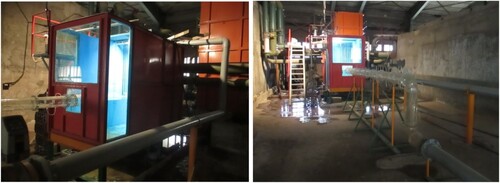
The experiments were studied in a laboratory tank 8.3 m³ (3.2 m of length, 1.3 m of width, and 2 m of height), facilitated with a closed-loop piping system (Figures 1 and 2). Five submerged depth/intake diameter (S/D) ratios (1, 1.5, 2, 2.5 and 3) were chosen to do the experiments such that a vortex usually forms. Tests were investigated at Five Froude numbers (Fr) (0.8, 1.0, 1.2, 1.4, and 1.6), which the water surface elevation in the tank could be monitored independently from flow discharge. These tests were performed nine trash racks with 63.7% to 84.1% opening, made of 2, 2.5, 4 and 6 mm thick copper wire. Experimental data has been performed with nine trash racks with 63.7% to 84.1% opening, made of 2, 2.5, 4 and 6 mm thick copper wire as an experence, two withdrawal directions (horizontal and 45°) were considered to monitor the impact of intake direction based on the hydraulic characteristics of the vortex. The PTV technique has been used for measuring the hydraulic characteristics of the vortex in planes perpendicular to the vortex axis. PTV analyses were carried out by implementing PTVlab code in MATLAB software. The Applied spherical tracer particles in the experiments are high-density polyethylene with a relative density of 0.041 and a diameter of 2 mm. The experimental set-up, particle detection method and the post-processing of the raw data are described in detail at the study of Aghajani et al. (2020).

Figure 1. A schematic illustration of the side view of the experimental model Aghajani et al. (2020).

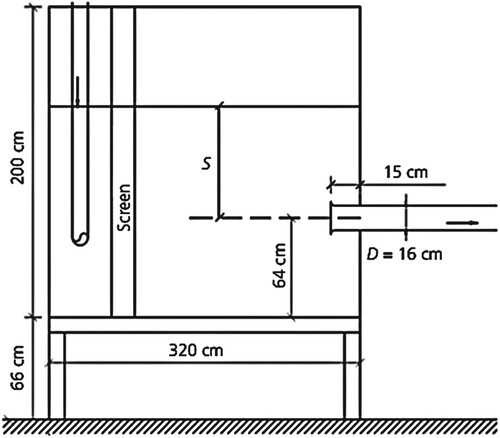
Figure 2. The experimental model.

Regression models

Random forest

As a supervised machine learning algorithm, Random Forest used for both classification and regression problems. This algorithm constructs decision trees on various instances and considers their majority vote for classification problems and the average for regression problems.

The ability of Random Forest algorithm to handle datasets containing both continuous variables for regression and categorical variables for classification is one of the most important features of this approach. It also often reveals better outcomes for classification problems.

In Random Forest, a number of samples are randomly selected from the dataset which has k number of records. Each sample corresponds to an individual decision tree, and each tree generates an output. The final output is achieved based on the majority voting or averaging for classification and regression respectively (Breiman, 2001; Geurts et al., 2006).

Recently, RF has been employed in numerous engineering applications because of its robust performance (Hasan & Horvat, 2024; Özen, 2024). In this paper, RF was employed to estimate the effect of trash racks on flow properties at power intakes.

KNN algorithm

KNN algorithm can be implemented for both classification and regression forecasting problems, with a focus on classification in industrial predictive scenarios. As a supervised machine learning method, KNN can be classified as a lazy learning algorithm because it does not require a predetermined training phase; instead, it utilizes the entire dataset for training to address classification and regression problems.

This algorithm benefits from ‘feature similarity’ to anticipate the values of new data points. Essentially, new data points are assigned values based on their proximity to the points in the training set, reflecting the degree of similarity between their features and those of the training data (Goldberger et al., 2004). The main parameters of KNN were determined through trial and error in this study. For instance, the number of neighbours was considered to be 5, and the metric for calculating the distance was set to Minkowski.

Gradient boosting (GB)

GB Regression is an ensemble learning method that applies multiple decision trees to improve the predictive performance of a model by iteratively adding new obtained trees to follow up the errors occurred through previous ones. The methodology of gradient boosting regression involves training a sequence of decision trees, in which each tree has been trained to minimize the residual errors of the previous tree. A weighted combination of all the participated trees in the ensemble can be considered as the final output.

Gradient boosting regression’s ability to deal with complex non-linear relationships among features and target variables is one of the main advantages of this algorithm. It is also robust to outliers and can handle a large number of features and observations. Additionally, gradient boosting can be easily parallelized, making it computationally efficient even on large datasets. Another advantage of gradient boosting is its ability to deal with missing data, which is a common problem with datasets in real-world. Furthermore, it is also less prone to overfitting compared to other models like random forest, as it builds trees one by one (Friedman, 2001; Hastie et al., 2009). Based on these advantages, the GB model was considered in the study for estimation of the effect of trash racks on flow properties at power intakes.

Lévy Jaya Algorithm (LJA)

Jaya is a Swarm Intelligence optimization algorithm that uses minimal number of parameters, population size and maximum number of generations, which is applied in many optimization domains in engineering practice (da Silva et al., 2023). The algorithm uses the position of solutions in the search space and updates it so the solutions would get updated to the best existed solution whereas it move away from the worst one (Rao, 2016).

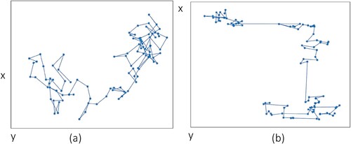
Lévy flight (Heidari & Pahlavani, 2017) is a type of random walk that is characterized by a probability density function that follows a power-law distribution. This means that the step size of the walk is not fixed, but rather follows a distribution where small steps are more likely than large steps. Figure 3 compares two-dimensional random walk and Lévy flight and illustrates the difference between the two patterns. A random walk has steps that are relatively similar in size, whereas a Lévy flight has small steps with occasional large steps.

Figure 3. A two-dimensional of random walk (a) vs. Lévy flight (b) (Iacca et al., 2021).

The Jaya algorithm is recognized for its tendency to become trapped in local optima during the search process. To address this issue, an enhanced version of the Jaya optimization algorithm, incorporating Lévy flight, was introduced (Iacca et al., 2021). The new version uses an action called ‘jump' for each particle in which enables it to move between various regions of the search space to begin a new local search. The problem of getting stuck in local optima would get solved through this approach and also it would be up to the mentioned process to monitor the balance between exploration and exploitation in the search process.

Proposed model

The proposed method for $N_t$ and $V_{\mathrm{xy}}/V_i$ estimation is shown in Figure 4 that $V_{\mathrm{xy}}$ is the flow velocity on the free surface of the water in plane x and y, and $N_t$ and $V_i$ are also explained in the introduction section. The flowchart outlines the process for training a gradient boosting (GB) regression model and evaluating its performance on $N_t$ and $V_{\mathrm{xy}}/V_i$ estimation. The process begins with data collection from two sources, $N_t$ and $V_{\mathrm{xy}}/V_i$. After normalization division of the collected data into three sets would get done as: a training set (60%), a validation set (20%), and a test set (20%).

Figure 4. Proposed method for $N_t$ and $V_{\mathrm{xy}}/V_i$ estimation.

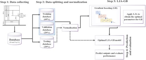
In order to find the optimal parameters of the GB model, LJA then would get applied to the training set. The optimized parameters are included as the number of estimators, the learning rate, the minimum number of leaf, and the maximum depth. By applying these optimal parameters, the GB model would get trained. At the end, the performance of the model would get evaluated on the test dataset through evaluation metrics (Section 2.4). Overall, the given flowchart would describe a process to train a GB model through LJA for optimization and evaluate its performance through a test dataset for $N_t$ and $V_{\mathrm{xy}}/V_i$ estimation.

Evaluation metrics

It is common to apply multiple metrics to obtain a comprehensive understanding of a regression model and its capabilities to monitor the performance of this specific model. Five different metrics were implemented including mean absolute error (MAE), mean squared error (MSE), root mean squared error (RMSE), R-squared ($R^2$), and Willmott’s index (WI) which are defined in Equations (3–7). These metrics offer various perspectives related to the performance of the model which can be implemented to distinguish strengths and weaknesses. Thus a clear picture of the model's overall performance would be provided through the mentioned metrics which can be implemented for further developments. (3) $\begin{array}{rl}\text{MAE}& =\frac{1}{n}\times \sum _{i=1}^n|y_i-{\hat{y}}_i|\end{array}$(3) (4) $\begin{array}{rl}\text{MSE}& =\frac{1}{n}\times \sum _{i=1}^n(y_i-{\hat{y}}_i{)}^2\end{array}$(4) (5) $\begin{array}{rl}\text{RMSE}& =\sqrt{\text{MSE}}\end{array}$(5) (6) $\begin{array}{rl}{R}^2& ={\left[\frac{{\sum }_{i=1}^n\left(y_i-\overline{y}\right).\left({\hat{y}}_i-{\overline{\hat{y}}}_i\right)}{\sqrt{{\sum }_{i=1}^n{\left(y_i-\overline{y}\right)}^2.{\left({\hat{y}}_i-{\overline{\hat{y}}}_i\right)}^2}}\right]}^2\end{array}$(6) (7) $\begin{array}{rl}\text{WI}& =1-\frac{{\sum }_{i=1}^n{\left(y_i-{\hat{y}}_i\right)}^2}{{\sum }_{i=1}^n{\left[\left(y_i-\overline{y}\right).\left({\hat{y}}_i-{\overline{\hat{y}}}_i\right)\right]}^2}\end{array}$(7)

In which y considered as the obtained value of a given variable, $\hat{y}$ depicts the predicted value of the previous variable, the number of observations is represented through n, $\overline{y}$ and $\overline{\hat{y}}$ are the average values of the mentioned variables.

Results

In this paper, four different regression models including GB, RF, KNN, and the proposed hybrid model, LJA-GB, are utilized for $N_t$ and $V_{\mathrm{xy}}/V_i$ estimation. The data is described in Section 2.1, and details about the implemented models are depicted in Tables 1 and 2.

Table 1. Initial parameters for GB, RF, and KNN models

Models	Parameter	Initial value
GB	Number of boosting stages to perform	100
	Learning rate	0.1
	The minimum number of samples required to be at a leaf node	1
	Maximum depth of individual regression estimators	3
RF	The number of trees in the forest	100
	The criterion to measure the quality of a split	Squared error
KNN	Number of neighbours	5
	Metric for distance computation	Minkowski
	Weights: weight function used in prediction	Uniform

Table 2. Optimal parameters of LJA-GB.

	Best parameters for GB obtained using LJA
Parameter	$N_t$	$V_{\mathrm{xy}}/V_i$
Number of boosting stages to perform	27	134
Learning rate	0.19	1.04
The minimum number of samples required to be at a leaf node	3	10
Maximum depth of individual regression estimators	17	15

Table 1 illustrates the initial parameters for three models: GB, RF, and KNN. GB has four parameters, RF has two parameters, and KNN has three parameters with initial values. The population size and the number of generations for LJA algorithm are set to 100.

Table 2 provides the optimal parameters for a GB model obtained using LJA method. The optimal values for $N_t$ estimation, in case of boosting stages to perform, learning rate, the minimum number of samples are supposed to be at a leaf node and for the maximum depth of individual regression estimators, respectively are summarized as 27, 0.19, 3 and 17. For $V_{\mathrm{xy}}/V_i$ estimation, the optimal values are: 134 for number of boosting stages to perform, 1.04 for learning rate, 10 for the minimum number of samples are considered to be at a leaf node and 15 for maximum depth of individual regression estimators. It is observed that the optimal values for GB parameters vary based on the estimation method used, $N_t$ and $V_{\mathrm{xy}}/V_i$ in this case.

Tables 3 and 4 present the performance of four models (GB, RF, KNN, and the proposed LJA-GB) in terms of five different evaluation metrics for both training and testing stages for two different estimations: $N_t$ and $V_{\mathrm{xy}}/V_i$.

Table 3. Comparison of evaluation metrics for $N_t$ estimation across four models

	Train					Test
Models	MAE	MSE	RMSE	$R^2$	WI	MAE	MSE	RMSE	$R^2$	WI
GB	0.0058	0.0001	0.0078	0.9964	0.9722	0.0083	0.0001	0.0117	0.9924	0.9622
RF	0.0053	0.0001	0.0099	0.9944	0.9748	0.014	0.0006	0.0239	0.9677	0.9339
KNN	0.0249	0.0014	0.0373	0.9338	0.8612	0.0300	0.0016	0.0400	0.9348	0.8331
LJA-GB	0.0040	0.0001	0.0071	0.9971	0.9810	0.0061	0.0001	0.0073	0.9971	0.9727

Table 4. $V_{\mathrm{xy}}/V_i$ estimation results across different models.

	Train					Test
Models	MAE	MSE	RMSE	$R^2$	WI	MAE	MSE	RMSE	$R^2$	WI
GB	0.1809	0.0651	0.2552	0.9957	0.9714	0.4102	0.262	0.5119	0.9856	0.9396
RF	0.6455	0.9196	0.959	0.9496	0.8849	0.8576	1.3128	1.1458	0.9384	0.8573
KNN	0.6464	0.8532	0.9237	0.952	0.8854	0.8596	1.2627	1.1237	0.943	0.8551
LJA-GB	0.0920	0.0165	0.1286	0.9989	0.9855	0.3344	0.1784	0.4223	0.9899	0.9508

For $N_t$ estimation, the LJA-GB model shows the best overall performance between the other four models evaluation, with the lowest MAE (0.0040, 0.0061), MSE (0.0001, 0.0001), and RMSE (0.0071, 0.0073) values and highest $R^2$ (0.9971, 0.9971) and WI (0.9810, 0.9727) values for both training and testing stages. The GB model also has a good performance with a low MAE (0.0058, 0.0083), MSE (0.0001, 0.0001), and RMSE (0.0078, 0.0117) and high $R^2$ (0.9964, 0.9924) and WI (0.9722, 0.9622) values for both training and testing stages. But the LJA-GB model has better performance than GB model. The RF model has a good performance for training stage with a low MAE (0.0053), MSE (0.0001), and RMSE (0.0099) and high $R^2$ (0.9944) and WI (0.9748) but its performance is a little bit worse for testing stage with higher values of MAE (0.014), MSE (0.0006), and RMSE (0.0239) and lower values of $R^2$ (0.9677) and WI (0.9339) than LJA-GB model. Lastly, the KNN model has the worst performance among the four models evaluated with higher values of MAE (0.0249, 0.0300), MSE (0.0014, 0.0016), and RMSE (0.0373, 0.0400) and lower values of $R^2$ (0.9338, 0.9348) and WI (0.8612, 0.8331) than LJA-GB model.

For $V_{\mathrm{xy}}/V_i$ estimation, the LJA-GB model shows the best overall performance among the four models evaluated, with the lowest MAE (0.0920, 0.3344), MSE (0.0165, 0.1784), and RMSE (0.1286, 0.4223) values and highest $R^2$ (0.9989, 0.9899) and WI (0.9855, 0.9508) values for both training and testing stages. The GB model also has a relatively good performance with a low MAE (0.1809), MSE (0.0651), and RMSE (0.2552) values for training stage but its performance is worse than LJA-GB model for testing stage with higher values of MAE (0.4102), MSE (0.262), and RMSE (0.5119) and lower values of $R^2$ (0.9856) and WI (0.9396) than LJA-GB model. The RF and KNN models have poor performance with high MAE (0.6455, 0.6464), MSE (0.9196, 0.8532), and RMSE (0.959, 0.9237) values and low $R^2$ (0.9496, 0.952) and WI (0.8849, 0.8854) values related to both training and testing phases.

In conclusion, based on the evaluation metrics presented in the tables, it is obvious that the proposed LJA-GB model has the best overall performance among the four models evaluated for both $N_t$ and $V_{\mathrm{xy}}/V_i$ estimations. The LJA-GB model has the lowest MAE, MSE, and RMSE values and highest $R^2$ and WI values for both training and testing stages for both estimations. Despite the acceptable performance of the GB model, the LJA-GB model has shown a better performance in both estimations. The other two models, namely RF and KNN have poor performance in the mentioned estimations.

The presented scatter plot in Figure 5 depicts the outcomes of four different regression models: GB, RF, KNN, and the proposed LJA-GB to estimate $N_t$. The results demonstrate that the LJA-GB model has the highest $R^2$ value of 0.9971 which shows a strong correlation among the predicted and actual values. The GB model has the second-highest $R^2$ value of 0.9924, leaded to the RF model with an $R^2$ value of 0.9679, and the KNN model with an $R^2$ value of 0.935. According to these findings it is highly s suggested that the LJA-GB model is the most precise model for predicting $N_t$ among the other four models evaluation.

Figure 5. Scatter plots of the observed and estimated $N_t$

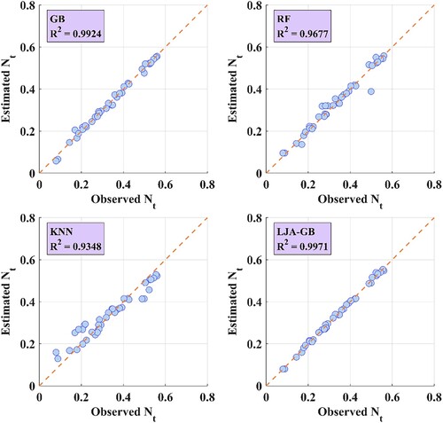
The scatter plot, in addition to the $R^2$ values, which includes the line $y=x$, that represents the ideal scenario, is able to make perfect estimations. Additional insights on the accuracy of the models can be provided through the location of the data points for each of the four models with respect to the line $y=x$. It is observed that the data points related to LJA-GB model are closest to the line $y=x$ in comparison with all the models which indicates the reality that LJA-GB model is making the most accurate estimations among the other four evaluated models. This would correspond to the high $R^2$ value of 0.9971. On the other hand, in case of other models, if the data points are farther away from the line $y=x$, it suggests that those models are less accurate.

Figure 6 presents the results of four different regression models: GB, RF, KNN, and proposed LJA-GB for the estimation of $V_{\mathrm{xy}}/V_i$. The results show that the LJA-GB model has the highest $R^2$ value of 0.9901, indicates a strong correlation among the predicted and actual values. It can be preserved that among the four evaluated models so far, the LJA-GB model has shown the best performance for predicting the value of $V_{\mathrm{xy}}/V_i$ . Moreover, the line $y=x$, is the dense area that the data points for LJA-GB model can be found there which considered as the ideal scenario of best estimations which provides more inevitable evidence of the superior performance of the LJA-GB model.

Figure 6. Scatter plots of the observed and estimated $V_{\mathrm{xy}}/V_i$

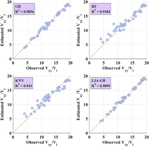
The scatter plots in 5 and Figure 6 depict the LJA-GB model shows the most effective in forecasting $N_t$ and $V_{\mathrm{xy}}/V_i$ between the other four evaluated models, since it has the highest $R^2$value and also the data points densely are located around the line of identity.

Figure 7 depicts both violin and box plots for the GB, RF, KNN, whereas in the meanwhile the proposed LJA-GB models for the estimation of $N_t$ and $V_{\mathrm{xy}}/V_i$ are presented. The distribution of data for each model and the summary of the distribution of data including the median, quartiles, and outliers respectively are depicted through violin and box plots. These mentioned plots provide additional information about the performance of the models.

Figure 7. Violin and box plot for $N_t$ and $V_{\mathrm{xy}}/V_i$

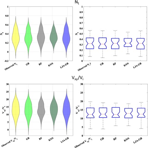
It can be observed through violin plot that the LJA-GB model has a smaller spread and a higher peak which indicate that the dense area of predicted values is located around the actual values, so it would lead to provide a better performance in comparison with the other models. The box plot also shows that the LJA-GB model has a smaller interquartile range and a higher median, indicating a more accurate performance.

In conclusion, Figure 7 provides additional evidence on the superior performance of the proposed LJA-GB model in comparison with the other models. The violin plots have depicted that the LJA-GB model has a smaller spread and a higher peak, which proves that the dense area of the predicted values is more concentrated around the actual values. Findings from the scatter plots in Figure 5 and Figure 6 confirm that the LJA-GB model is the most precise in predicting $N_t$ and $V_{\mathrm{xy}}/V_i$ among the other four models evaluated.

Which uses as an approach in order to visualize the performance of various models in terms of correlation and RMSE, Figure 8 depicts the Taylor diagram. It also depicts the GB, RF, KNN along with the proposed LJA-GB models which are plotted on the diagram. Hence from the Taylor diagram, it can be understood that the LJA-GB model has the closest estimation to the ground truth, which represents the most fitted scenario which indicate its high correlation and the lowest RMSE among the other four models. It confirms that the LJA-GB model is the best approach among the entire presented models which are evaluated in terms of correlation and accuracy.

Figure 8. Taylor diagram for $N_t$ and $V_{\mathrm{xy}}/V_i$

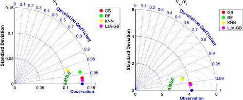
In conclusion, the results presented in the scatter plots, Taylor diagram, box plot, and violin plot all demonstrate that the proposed LJA-GB model is the most effective in predicting $N_t$ and $V_{\mathrm{xy}}/V_i$ among the four models evaluated. The scatter plots show that the LJA-GB model has the highest $R^2$ value and the data points are closest to the line of identity, corresponds to a strong correlation among the predicted and observed values. The Taylor diagram demonstrates that the LJA-GB model has the highest correlation and the lowest RMSE among the four models, indicating the best performance in terms of correlation and accuracy. The box plot and violin plot also show that the LJA-GB model has a smaller spread and a higher peak, indicating that the predictions are more concentrated around the ground truth. All these figures clearly indicate that LJA-GB model is the best performer among the models evaluated in terms of correlation and accuracy.

Friedman test

The performance of the standalone and hybrid models is assessed using statistical tests on six test datasets through cross-validation on $N_t$ and $V_{\mathrm{xy}}/V_i$ data (D1–D6). The Friedman test evaluates significant differences in model performance based on MAE values, comparing the distribution of treatments. If the null hypothesis is rejected, we proceed to evaluate model performance with the alternative hypothesis. The MAE values were obtained from four different models on test datasets is shown in Table 5. The ranking table for Friedman test was calculated which are in the form 1 to k that 1 represents to the lowest MAE and k represents the highest value of MAE. Then, the average of rank for each model obtained which is demonstrated in Table 6. The Friedman test statistics is given as (Demšar, 2006): (8) $\begin{array}{r}{\chi }^2=\frac{12n}{k\left(k+1\right)}\left[\sum _{i=1}^{k}A{R}_j^2-\frac{k{\left(k+1\right)}^2}{4}\right]\end{array}$(8) where n, k, and ${\chi }^2$ represent the number of datasets, models, and chi-square distribution respectively. The calculated ${\chi }^2$ is compared with the critical value. If the ${\chi }^2$ is larger than the critical value, the null hypothesis is rejected; if the ${\chi }^2$ is less than the critical value, the null hypothesis is not rejected. The Friedman test statistic (18) exceeds the critical value (7.815) at a significance level of 0.05, indicating a significant difference between the proposed model and the utilized models. In this analysis, the analysis reveals the superiority of the LJA-GB model over the others utilizing six random datasets from the original data. This significant difference in the Friedman test underscores the superior performance of the proposed model compared to other models.

Table 5. Performance of applied models on test datasets in terms of MAE value.

Metrics	D1	D2	D3	D4	D5	D6
GB	8.316	7.896	10.657	0.41	0.399	0.369
SVM	14.517	10.825	14.521	0.586	0.459	0.452
KNN	30.906	29.769	27.186	0.881	0.766	0.901
LJA_GB	5.68	5.536	8.427	0.31	0.33	0.328

Table 6. Friedman test ranks.

Metrics	D1	D2	D3	D4	D5	D6	AR
GB	2	2	2	2	2	2	2
SVM	3	3	3	3	3	3	3
KNN	4	4	4	4	4	4	4
LJA_GB	1	1	1	1	1	1	1

Conclusion

This paper was aimed to approximate $N_t$ and $V_{\mathrm{xy}}/V_i$ to study the effect of the trash rack on flow properties at power intakes. First, estimation was obtained using three machine learning models: GB, RF, and KNN. Next, a novel hybrid model was employed to improve the estimation for $N_t$ and $V_{\mathrm{xy}}/V_i$. To this aim, the LJA optimization algorithm was coupled with GB (i.e. LJA-GB). A comparison of the proposed hybrid LGA-GB with the other implemented machine learning models demonstrated its enhanced estimation accuracy. Overall, the hybrid LJA-GB model achieved the best estimation in both the $N_t$ and $V_{\mathrm{xy}}/V_i$ scenarios. The LJA-GB model obtained the MAE (0.0920, 0.3344), MSE (0.0165, 0.1784), RMSE (0.1286, 0.4223), $R^2$ (0.9989, 0.9899), and WI (0.9855, 0.9508) for $V_{\mathrm{xy}}/V_i$ estimation in the training and testing phases. Moreover, the LJA-GB model obtained the MAE (0.0040, 0.0061), MSE (0.0001, 0.0001), and RMSE (0.0071, 0.0073) values and $R^2$ (0.9971, 0.9971) and WI (0.9810, 0.9727) values for both training and testing stages for $N_t$ estimation.

It should be noted the data used for training and testing the models likely originated from a specific laboratory setup. The accuracy of the models for real-world power plant intakes might require further validation. The study could be strengthened by incorporating data from various trash rack configurations and real-world power plant settings. Sensitivity analysis could be performed to understand how the model predictions change based on different input parameters (e.g. water flow rate, trash rack clogging level). Exploring alternative machine learning models or incorporating feature engineering techniques might potentially improve estimation accuracy.

Based on findings in the presented research, no prior research has employed the hybrid LJA-GB model to estimate $N_t$ and $V_{\mathrm{xy}}/V_i$. As highlighted in the paper, developing other hybrid models by combining different machine learning algorithms with various optimization techniques is a promising avenue for future research. The LJA-GB model could be used to predict flow properties for other types of hydraulic structures beyond power plant intakes. The research could be extended to investigate the impact of trash rack clogging or debris accumulation on flow characteristics and model performance.

Disclosure statement

No potential conflict of interest was reported by the author(s).

References

- Aghajani, N., Karami, H., Sarkardeh, H., & Mousavi, S. F. (2020). Experimental and numerical investigation on effect of trash rack on flow properties at power intakes. ZAMM-Journal of Applied Mathematics and Mechanics/Zeitschrift für Angewandte Mathematik und Mechanik, 100(9), e202000017. https://doi.org/10.1002/zamm.202000017
- Azarpira, M., & Zarrati, A. R. (2019). A 3D analytical model for vortex velocity field based on spiral streamline pattern. Water Science and Engineering, 12(3), 244–252. https://doi.org/10.1016/j.wse.2019.09.001
- Azarpira, M., Zarrati, A., Farokhzad, P., & Shakibaeinia, A. (2022). Air-core vortex formation in a draining reservoir using smoothed-particle hydrodynamics (SPH). Physics of Fluids, 34(3), 037101. https://doi.org/10.1063/5.0077083
- Azarpira, M., Zarrati, A. R., & Farrokhzad, P. (2021). Comparison between the Lagrangian and Eulerian approach in simulation of free surface air-core vortices. Water, 13(5), 726. https://doi.org/10.3390/w13050726
- Breiman, L. (2001). Random forests. Machine Learning, 45(1), 5–32. https://doi.org/10.1023/A:1010933404324
- Chang, L., & Wei, W. (2023). Numerical study on the effect of tangential intake design and inflow discharge on vertical dropshaft assessment using pressure and velocity distributions. Engineering Applications of Computational Fluid Mechanics, 17(1), 2252045. https://doi.org/10.1080/19942060.2023.2252045
- da Silva, L. S. A., Lúcio, Y. L. S., d, L., Coelho, S., Mariani, V. C., & Rao, R. V. (2023). A comprehensive review on Jaya optimization algorithm. Artificial Intelligence Review, 56(5), 4329–4361. https://doi.org/10.1007/s10462-022-10234-0
- Demšar, J. (2006). Statistical comparisons of classifiers over multiple data sets. The Journal of Machine Learning Research, 7, 1–30.
- Friedman, J. H. (2001). Greedy function approximation: A gradient boosting machine. Annals of Statistics, 29(5), 1189–1232.
- Geurts, P., Ernst, D., & Wehenkel, L. (2006). Extremely randomized trees. Machine Learning, 63(1), 3–42. https://doi.org/10.1007/s10994-006-6226-1
- Goldberger, J., Hinton, G. E., Roweis, S., & Salakhutdinov, R. R. (2004). Neighbourhood components analysis. Advances in Neural Information Processing Systems, 17, 513–520.
- Hasan, J., & Horvat, M. (2024). An application of the random forest algorithm for the prediction of Solar Envelope ‘Floor Space Index’ based on spatiotemporal parameters. Journal of Building Engineering, 86, 108784. https://doi.org/10.1016/j.jobe.2024.108784.
- Hastie, T., Tibshirani, R., Friedman, J. H., & Friedman, J. H. (2009). The elements of statistical learning: Data mining, inference, and prediction. Springer.
- Heidari, A. A., & Pahlavani, P. (2017). An efficient modified grey wolf optimizer with Lévy flight for optimization tasks. Applied Soft Computing, 60, 115–134. https://doi.org/10.1016/j.asoc.2017.06.044
- Iacca, G., dos Santos Junior, V. C., & de Melo, V. V. (2021). An improved Jaya optimization algorithm with Lévy flight. Expert Systems with Applications, 165, 113902. https://doi.org/10.1016/j.eswa.2020.113902
- Kan, K., Xu, Y., Li, Z., Xu, H., Chen, H., Zi, D., Gao, Q., &Shen, L. (2023). Numerical study of instability mechanism in the air-core vortex formation process. Engineering Applications of Computational Fluid Mechanics, 17(1), 2156926. https://doi.org/10.1080/19942060.2022.2156926
- Khanarmuei, M., Rahimzadeh, H., & Sarkardeh, H. (2019). Effect of dual intake direction on critical submergence and vortex strength. Journal of Hydraulic Research, 57(2), 272–279. https://doi.org/10.1080/00221686.2018.1459896
- Monshizadeh, M., Tahershamsi, A., Rahimzadeh, H., & Sarkardeh, H. (2017). Comparison between hydraulic and structural based anti-vortex methods at intakes. The European Physical Journal Plus, 132(8), 1–11. https://doi.org/10.1140/epjp/i2017-11608-4
- Özen, F. (2024). Random forest regression for prediction of Covid-19 daily cases and deaths in Turkey. Heliyon, 10(4), 1–19.
- Rao, R. (2016). Jaya: A simple and new optimization algorithm for solving constrained and unconstrained optimization problems. International Journal of Industrial Engineering Computations, 7(1), 19–34.
- Sarkardeh, H. (2017). Minimum reservoir water level in hydropower dams. Chinese Journal of Mechanical Engineering, 30(4), 1017–1024. https://doi.org/10.1007/s10033-017-0156-7
- Sarkardeh, H., Jabbari, E., Zarrati, A. R., & Tavakkol, S. (2014). Velocity field in a reservoir in the presence of an air-core vortex. Proceedings of the Institution of Civil Engineers-Water Management, 167(6), 356–364. https://doi.org/10.1680/wama.13.00046
- Sarkardeh, H., & Marosi, M. (2022). An analytical model for vortex at vertical intakes. Water Supply, 22(1), 31–43. https://doi.org/10.2166/ws.2021.288
- Sarkardeh, H., Zarrati, A. R., & Roshan, R. (2010). Effect of intake head wall and trash rack on vortices. Journal of Hydraulic Research, 48(1), 108–112. https://doi.org/10.1080/00221680903565952
- Taştan, K., & Yildirim, N. (2010). Effects of dimensionless parameters on air-entraining vortices. Journal of Hydraulic Research, 48(1), 57–64. https://doi.org/10.1080/00221680903566018