A novel spatial–temporal prediction method for the effects of fish movement on flow field based on hybrid deep neural network

Abstract

In the fish passage facility design, understanding the coupled effects of hydrodynamics on fish behaviour is particularly important. The flow field caused by fish movement however are usually obtained via time-consuming transient numerical simulation. Hence, a hybrid deep neural network (HDNN) approach is designed to predict the unsteady flow field around fish. The basic architecture of HDNN includes the UNet convolution (UConv) module and the bidirectional convolutional long-short term memory (BiConvLSTM) module. Specifically, the UConv module extracts crucial features from the flow field graph, while the BiConvLSTM module learns the evolution of low-dimensional spatio-temporal features for prediction. The numerical results showcase that the HDNN achieves accurate multi-step rolling predictions of the effect of fish movement on flow fields under different tail-beat frequency conditions. Specifically, the average and standard deviation of PSNR and SSIM for the proposed HDNN model for 60 time-step rolling predictions on the entire sequences of four test sets being respectively larger than 34 dB and 0.9. The HDNN delivers a speedup of over 130 times compared to the numerical simulator. Moreover, the HDNN demonstrates commendable generalisation capabilities, enabling the prediction of spatial–temporal evolution within unsteady flow fields even at unknown tail-beat frequencies.

KEYWORDS:

• Unsteady flow prediction
• fluid-structure interaction
• deep neural network
• fish

1. Introduction

River restoration is currently a hot topic in water resources research (Wohl et al., 2015). Fish, as important members of river systems, are interconnected in the study of relationships between the entire flow regime, biological communities, and ecosystem processes (Palmer & Ruhi, 2019). The construction of numerous hydropower projects has led to river fragmentation, significantly impacting fish habitat and migration behaviours. The construction of fish passage facilities in hydraulic engineering is an effective means of restoring river connectivity. These fish passage facilities can help fish cross obstacles posed by hydraulic engineering, enabling them to migrate smoothly, find habitats, search for food, and spawn. This helps alleviate the impact of hydraulic engineering on fish ecosystems. However, fish migration is a complex process involving the coupled effects between changing hydraulic indicators and fish behaviour. If the design of fish passage facilities does not consider the detailed coupled effect and simply mimics the natural flow conditions, it may be challenging to ensure the smooth migration of fish.

Currently, extensive research has been conducted discussing the impact of various hydrodynamic indicators on fish behaviour (Liu et al., 2023a; Silva et al., 2020). Among these indicators, flow velocity is a crucial factor that can serve as a source of navigation information during the migration process. For instance, Liu et al. (2023a) found that Schizothorax wangchiachii exhibits active selection or avoidance behaviour in high-flow areas (1.6–1.8 m/s). Wang et al. (2023) discovered that flow direction can be a crucial predictive factor for deducing the upstream trajectory of juvenile Schizothorax prenanti when passing through fishways, and the predicted trajectory aligns well with actual observations. Furthermore, hydrodynamics not only influence the activities of individual but also play a crucial role in schooling mechanisms. Relevant studies indicate that within a school of fish, the vortical energy generated by the leading fish can be harnessed by those following closely behind. This allows individuals in the group to reduce swimming effort and move forward continuously (De Bie et al., 2020; Liao et al., 2003). Therefore, understanding the coupled effects of hydrodynamics on fish swimming behaviour is particularly important for the design of ecological conservation projects.

To further explore the principles behind fish swimming behaviour related to hydrodynamics, numerous researchers have conducted studies on the hydrodynamic interactions using numerical simulation techniques (Khalid et al., 2018; Kong et al., 2018; Li et al., 2022a; Rui et al., 2023; Wei et al., 2022). Typically, the problems of fluid-structure interaction (FSI) are solved by solving the Navier-Stokes (NS) equations, known as computational fluid dynamics (CFD). Li et al. (2022b) employed CFD methods to numerically simulate the viscous fluid around a biomimetic dolphin. They analyzed quantitative fluid dynamics issues behind specific motion patterns, including movement velocity, energy loss, and operational efficiency. Liu et al. (2023b) used a CFD-based fluid-structure coupled model to study the interaction between fish movement and flow fields, quantitatively analyzing the impact of different numbers of fish on the flow field in aquaculture ponds. Chen et al. (2016) utilised CFD methods to examine thrust enhancement and energy savings in three stable swimming fish, with one fish upstream and two fish downstream. By controlling the longitudinal and lateral distances between fish, they investigated the complex interactions among fish in a school, demonstrating the hydrodynamic interactions between shedding vortices and undulating fish bodies.

The aforementioned studies indicate that the CFD method can well simulate the interaction between fish movement and flow field. However, it is a time-consuming process, which needs large computing resources for extensive numerical computation. Therefore, there is a need for a robust method that can predict fluid dynamics faster than CFD simulations. With the advancements in computer science and machine learning theory, the field of data processing has experienced significant development (Meng et al., 2023). Deep learning (DL) technology has been explored in the field of fluid mechanics to achieve efficient and effective flow field prediction, control, and optimisation (Fukagata et al., 2019; Zhong et al., 2023). For instance, DL has been applied to data-driven steady flow reconstruction due to its computational accuracy and efficiency. Guo et al. (2016) proposed a universal and flexible approximation model based on convolutional neural networks (CNN) for real-time prediction of non-uniform steady laminar flow in a two-dimensional (2D) or three-dimensional (3D) domain. This approach is four orders of magnitude faster than CPU-based CFD solvers. Compared to multi-layer perceivers, multi-head perceivers achieve better predictions for sparse flow fields. Cai et al. (2022) simulated the velocity field of vacuum plumes using CNN, and the predicted results aligned well with the numerical simulation results obtained through direct simulation Monte Carlo methods, with an acceleration factor of up to four orders of magnitude. In addition to accelerating steady flow field solutions, DL is equally applicable to rapidly solving unsteady flow fields. Han et al. (2019) designed a novel hybrid deep neural network to capture spatio-temporal features of unsteady flows directly from high-dimensional numerical unsteady flow field data. The network demonstrated promising potential in modelling spatio-temporal flow features. Eivazi et al. (2020) proposed a convolutional autoencoder long short-term memory (CAE-LSTM) method for reduced-order modelling of the unsteady fluid flows, which can well predict fluid flow evolution.

It can be seen from the above that some scholars have employed different feature extraction methods to reconstruct flow fields for both steady and unsteady conditions. However, the majority of current methods for reconstructing and predicting unsteady flow fields using neural networks are predominantly utilised in scenarios without considering FSI, whose flow characteristics exhibit minimal variations and complexity is much simpler than the FSI flow field with strong discontinuous nonlinear and complex spatial–temporal characteristics. For the flow field around fish, it is much more challenging than linear flow fields to establish a neural network to make flow field analysis and prediction. To the best of the authors’ knowledge, there are no publicly available reports on neural network modelling for the hydrodynamic interaction between flow and fish behaviour in the available public literature.

Learning the unsteady flow dynamics around fish directly represents a valuable yet challenging approach. To address the task of efficiently modelling the complex unsteady flow field influenced by fish behaviour, a hybrid deep neural network (HDNN) approach is designed to predict the unsteady flow. The basic architecture of HDNN includes the UNet convolution (UConv) module and the bidirectional convolutional long-short term memory (BiConvLSTM) module. Specifically, the UConv module extracts crucial features from the flow field graph, while the BiConvLSTM module learns the evolution of low-dimensional spatio-temporal features for prediction.

This study explores, for the first time, the feasibility of using DL for predicting the effect of fish behaviour on fluid dynamics, focusing on the cyprinid fish. By employing CFD numerical simulations and data processing, a time-series dataset of flow fields is established. Through model training and testing, the performance and efficiency of the proposed HDNN are investigated. The results indicate that the proposed HDNN framework demonstrates superior generalisation and prediction capability for the complex unsteady flow field characteristics. This validates the potential of the developed model for data-driven modelling and prediction application in complex unsteady FSI flow fields. Additionally, compared with traditional CFD, HDNN dramatically reduces the simulation time and still has high accuracy, showing HDNN is a promising method for the simulation of FSI dynamics.

This paper is organised as follows. Section 2 introduces the details of preparing the dataset, Section 3 presents the construction of HDNN, including the overall architecture of the network, the methods for model training and prediction, and evaluation metric. Section 4 shows and discusses the predictive performance results of HDNN. Section 5 presents the concluding of the study.

2. Dataset generation

2.1. CFD simulation of fluid dynamics

CFD numerical simulations have been successfully applied to reveal the flow characteristics of the effect of fish behaviours on flow field (Li et al., 2022c; Tang et al., 2017; Zhao & Shi, 2023). This work uses CFD due to its excellent computational capability. The details of the model are provided below.

2.1.1. Computational model

In order to reduce computational complexity and generate more numerical simulation data, a Lagrangian coordinate system is employed to describe the motion of fish. In this description, the origin of the coordinate system is always located at the centre of the fish, and the flow velocity is represented in relative terms, denoted as $V_{\text{flow}}^{\mathrm{\prime }}$. (1) $V_{\text{flow}}^{\mathrm{\prime }}=V_{\text{flow}}+V_{\text{swim}},$(1) where, $V_{\text{flow}}$ is the absolute flow velocity, m/s; $V_{\text{swim}}$ is the absolute swimming speed of the fish, m/s.

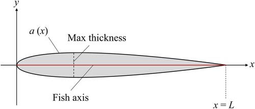
In this study, the 2D smooth contour of the fish is generated using a curve-fitting method (Wang & Wu, 2010). The configuration of the fish-shaped body is a streamlined region in the x-y plane, with its axis of symmetry located along the x-axis. The tail and head are positioned at (0, 0) and (L, 0), respectively. The contour is approximated by a quadratic curve in the form of an amplitude envelope $a(x)$ as follows: (2) $a(x)=a_0+a_{1}x+a_2{x}^2,$(2) where, $a_i$ represents the coefficients of the envelope line, where i ranging from 0 to 2. When the coefficients are $a_0$ = 0.02, $a_1$ =  – 0.08, and $a_2$ = 0.16, the resulting reference configuration is illustrated in Figure 1. L denotes the length of the fish body, with L = 0.1 m in this study.

Figure 1. Reference shape of the cyprinid fish. The contours $\pm a(x)$ are parametrised by eq. (2).

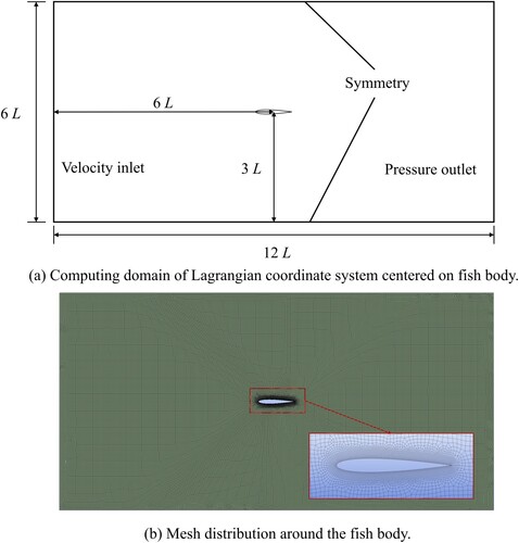
The domain and grids used for numerical simulation are established based on computational cost and accuracy. The entire swimming area is represented by a rectangular zone of dimensions 12 L × 6 L, filled with water, as shown in Figure 2 (a). The boundary conditions are set as follows: the inlet is set to a velocity inlet, and the inlet velocity is $V_{\text{flow}}^{\mathrm{\prime }}$ (specific values depend on different simulation conditions, as indicated in the subsequent table); the outlet is set to a pressure outlet; the upper and lower sides are set to symmetrical planes; the surface of the fish is applied to no-slip condition. The inlet and outlet are both 6 L from the centre of the fish; the upper and lower sides are both 3 L from the centre of the fish.

Figure 2. Diagram of the numerical model.

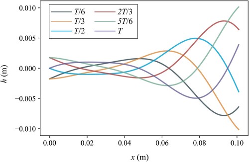
In this study, the swimming style of cyprinid fish is used as the reference. The kinematics of cyprinid fish typically exhibit a backward travelling wave form with maximum amplitude at the tail. The specific kinematics used in this work are based on experimental observations by Videler and Hess (1984). The lateral oscillation of the fish body is expressed as follows: (3) $h(x,t)=a(x)\text{sin}(\mathrm{kx}-\mathrm{\omega t}),$(3) where, $k=2\pi /\lambda$ is the wave number corresponding to the wavelength $\lambda$ of the main body oscillation; $\omega =2\pi f$ is the angular frequency corresponding to the tail-beat frequency $f$, which is calculated based on the empirical formula eq. (4(4) $V_{\text{swim}}=0.71\mathrm{fL},$(4) ) from Curatolo and Teresi (2015). The wave number $k$ in the simulation is based on the dimensionless wavelength $\lambda /L=$95%, which falls within the observed range of 89–110% in most carangiform swimmers. Figure 3 displays the axial motion $h(x,t)$ at six different instants within one beating period T. (4) $V_{\text{swim}}=0.71\mathrm{fL},$(4)

Figure 3. Mid-line motions of chordwise fish body in one beating period.

2.1.2. Numerical method

To simulate the 2D viscous fluid around fish, this study employs the following NS equations to define the relevant governing equations: (5) $\begin{array}{rl}\mathrm{\nabla }\cdot u& =0,\end{array}$(5) (6) $\begin{array}{rl}\rho \frac{\mathrm{\partial }u}{\mathrm{\partial }t}+\rho (u\cdot \mathrm{\nabla })u& =-\mathrm{\nabla p}+\mu {\mathrm{\nabla }}^{2}u,\end{array}$(6) where $\mathrm{\nabla }$ is the gradient operator, $\rho$ is the density, $p$ is the pressure divided by the density and $\mu$ is the dynamic viscosity.

The simulation is conducted in the computational domain, as shown in Figure 2 (a). Fluent Meshing is employed to discretize the entire fluid domain in Figure 2 (b) into quadrilateral grids, with inflation operations and refinement applied around the fish body. The Fluent solver serves as the CFD tool during the simulation process. The solution of the pressure-velocity coupled continuity equation utilises the SIMPLE algorithm, and the turbulence models adopt the RNG $k$-ϵ equation. In the numerical calculation of fluid-structure coupling, the embedded DEFINE_GRID_MOTION macro is connected to the main code of the solver to realise the required flexible deformation motion. The time-step of the numerical simulation is set based on the fish’s tail-beat frequency, calculated using the empirical formula eq. (7(7) $\mathrm{\Delta }t=0.001\frac{1}{f},$(7) ), in order to avoid negative cell volume during the simulation. (7) $\mathrm{\Delta }t=0.001\frac{1}{f},$(7) where $\mathrm{\Delta }t$ represents the time-step of the numerical simulation.

2.2. Dataset constructions

Dataset construction is a crucial aspect of DL for achieving better training and predictive performance. To evaluate the effectiveness of the proposed model, this study designs three cases for testing. This section covers case descriptions and data processing.

2.2.1. Case description

In order to validate the adaptability of the model, this study designs three representative experiments by changing the tail-beat frequency and the corresponding relative flow velocity ($V_{\text{flow}}^{\mathrm{\prime }}$) to predict the FSI flow fields.

The absolute flow velocity ($V_{\text{flow}}$) is set to 0.02 m/s for all three experiments. The specific settings for the CFD numerical simulations in the three cases are provided in Table 1. The first numerical experiment (Case 1) involves 2D flow during slow swimming of the fish at $f$ =  0.4 Hz. The second experiment (Case 2) represents 2D flow during fast swimming of the fish at $f$ = 3 Hz. The third experiment (Case 3) is intended to evaluate the generalisation ability of the neural network. In Case 3, the training dataset for the network includes 2D flow field data at $f$ =  0.5, 0.6, 0.7, 0.8, 0.9, and 1 Hz. These datasets are denoted as Case 3-1, Case 3-2, Case 3-3, Case 3-4, Case 3-5, and Case 3-6, respectively, capturing potential dynamics within the tail-beat frequency range from 0.5–1 Hz. The datasets for testing involve $f$ = 1.1 and 0.65 Hz, referred to as Case 3–7 and Case 3-8.

Table 1. Parameter settings for numerical simulation of different cases.

Case	$V_{\text{flow}}$(m/s)	$V_{\text{swim}}$(m/s)	$V_{\text{flow}}^{\mathrm{\prime }}$(m/s)	$f$ (Hz)
Case 1	0.02	0.028	0.048	0.4
Case 2	0.02	0.213	0.233	3
Case 3–1	0.02	0.035	0.055	0.5
Case 3–2	0.02	0.043	0.063	0.6
Case 3–3	0.02	0.05	0.07	0.7
Case 3–4	0.02	0.057	0.077	0.8
Case 3–5	0.02	0.064	0.084	0.9
Case 3–6	0.02	0.071	0.091	1
Case 3–7	0.02	0.078	0.098	1.1
Case 3–8	0.02	0.046	0.066	0.65

Note: $V_{\text{flow}}$ is the absolute flow velocity; $V_{\text{swim}}$ is the absolute swimming speed of the fish; $V_{\text{flow}}^{\mathrm{\prime }}$ is the relative flow velocity in the Lagrangian coordinate system; $f$ is the tail-beat frequency of the fish. The values for the velocity boundary conditions in the numerical simulations are determined based on $V_{\text{flow}}^{\mathrm{\prime }}$.

2.2.2. Data processing

Since the CNN is developed from the field of computer vision, the objective of HDNN is to predict flow fields at future occasions based on the temporal history of flow fields. The approach is similar to the image-to-image regression tasks considered in DL. Therefore, the datasets used to train and test the network should resemble image datasets, where the information values of each moment’s flow field should be distributed over a grid of uniform points, such as pixels.

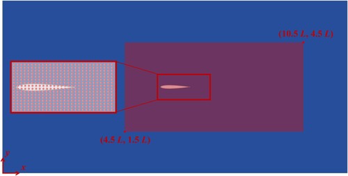
In the work, a rectangular area is arranged near the fish body as the sampling area, as shown in Figure 4, covering the spatial range from (4.5, 1.5 L) to (10.5, 4.5 L). Sampling points of 100 × 200 are placed in the sampling area (area with the colour red). The flow field variables are projected onto the sampling points, and the 2D flow field variables ($V_x$ and $V_y$) are extracted. The values of the point inside the body are 0. Considering the periodic wake caused by the varying tail-beat frequencies for three cases, the sampling interval is adjusted to ensure that each tail-beat cycle contains approximately 60 time-steps. Additionally, the unstable flow field during the initial phase (0–10 s) is discarded due to its adverse impact on model training. The extracted 100 × 200 × 2 dimensional data represent each instantaneous field.

Figure 4. The sampling area around the fish body.

The extracted data is arranged in chronological order to create a dataset describing the temporal evolution of the flow field. The data for the temporal evolution of the flow field at each time-step consists of a snapshot with dimensions (1, 2, 100, 200), where (1, 2, 100, 200) denotes one snapshot, two flow field variables, and spatial resolution of the sampling area (100, 200). Moreover, to predict data of flow fields at time-step $t$ from data at time-steps $t\text{--}k+1$ to $t\text{--}1$, the dataset needs to be divided into time sequences. Considering the limitation of GPU memory for predicting the length of time, each training pass into the CNN involves $k=10$snapshots, i.e. (10, 2, 100, 200). The obtained data is arranged in chronological order to form a dataset describing the temporal evolution of the flow field. For Case 1 and Case 2, datasets containing 2000 time-steps were obtained, representing approximately 34 cycles with 2000 consecutive flow field computations. Among these, 1820 time-steps were used as the training set, and 180 time-steps were used as the test set. For Case 3, under 8 different $f$ conditions, each condition resulted in 300 time-steps, totalling 2400 time-steps. Case 3–1 to Case 3–6 constituted the training set with a total of 1800 time-steps, while Case 3–7 and Case 3–8 formed the test set with a total of 600 time-steps. This represents approximately 40 cycles with 2400 consecutive flow field computations in Case 3.

Finally, the training set and testing set are normalised for better accuracy. This approach circumvents the inclusion of extraneous information in the training samples, thereby benefiting the training process and feature extraction.

3. HDNN: the deep spatio-temporal sequence model for the fluid dynamics

3.1. Model architecture of HDNN

The transient response of flow field in the process of unsteady flow is related to the historical development. This implies that the flow at the next moment is influenced by the evolution of the current moment and even previous historical moments. Hence, this section attempts to establish a spatio-temporal model for predicting the 2D flow fields around fish. The challenges here however include (1) large-scale 2D graph learning and (2) learning the underlying spatio-temporal dynamics.

3.1.1. UConv module: large-scale 2D graph learning

To tackle the challenge of efficiently learning from extensive 2D fluid graphs, the convolution module of UNet (UConv) is employed, which is responsible for extracting important features from the large-scale 2D graph. UNet was initially proposed by Ronneberger et al. (2015) for medical image segmentation tasks and has been successfully applied in flow field reconstruction in recent years (Cai et al., 2022; Li et al., 2023). In comparison to the classical convolutional autoencoder (Guo et al., 2016), UConv stands out by utilising the output of the convolution in the encoding part as the input for the corresponding deconvolution at the same position in the decoder. This operation is crucial for effectively recovering lost information during the convolution process and avoiding the issue of gradient vanishing.

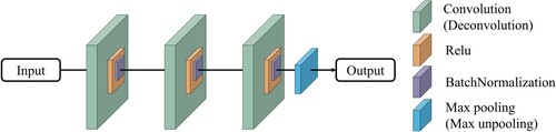
Specifically, the downsampling encoder network of UConv module, consisting of connected convolution blocks, are designed to capture complex spatial features directly from the high-dimensional input field and represent them in a low-dimensional form. The upsampling decoder network replicates the downsampling encoder network architecture and reverses it, consisting of deconvolution blocks. Its purpose is to represent the predicted lowdimensional feature maps to high-dimensional output field, with the same dimension as input fields. Each convolution or deconvolution block includes three convolution or deconvolution layers and max pooling or max unpooling layers, as shown in Figure 5. A single convolution or deconvolution layer involves the processes of convolution or deconvolution, ReLU activation, and batch normalisation.

Figure 5. Architecture of a single convolution or deconvolution block.

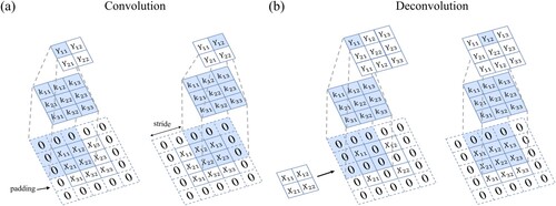
Through the convolutional layers, the encoder maps the large-size input data to small-size feature maps, so that the CNN ‘learns’ the features in the input data. The convolution process is illustrated in Figure 6 (a). In the given example, with a kernel size of 3 and a stride of 2, zero-padding is applied at the boundaries of the input data to maintain the original matrix shape. The deconvolution process is the inverse operation of convolution in Figure 6 (b).

Figure 6. Schematic of (a) convolution operation concept and (b) deconvolution. $X_{\mathrm{ij}}$ shows the input, $k_{\mathrm{ij}}$ is the convolution kernel, and $Y_{\mathrm{ij}}$ shows the output.

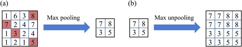
Batch normalisation is introduced to fix the mean and variance of each layer’s input, making the network train faster and more stable. Figure 7 illustrates the max pooling process. Max pooling is essentially a downsampling operation, where the maximum value of patches in the input matrix is calculated and used to create the downsampled matrix. In this paper, the patch size is 2, implying that after the max pooling process, the length and width of the input matrix are halved. The max unpooling process is the inverse operation of max pooling.

Figure 7. Schematic of (a) max pooling and (b) max unpooling layer.

3.1.2. BiConvLSTM module: unstructured spatio-temporal learning

Considering the inherent flow dynamics, the current flow field is correlated with the previous moment’s flow field, indicating a strong continuity in the temporal scale of the flow field. To address the challenge of learning the underlying spatio-temporal dynamics, the BiConvLSTM module is employed to capture the temporal.

Traditional LSTM networks are specialised in capturing temporal characteristics. A typical LSTM cell comprises three gates: the input gate, the output gate, and the forget gate. The LSTM cell regulates the flow of training information through these gates by selectively adding information (input gate), removing information (forget gate), or letting it through to the next cell (output gate). LSTM networks utilise their internal memory, ensuring predictions are conditioned on recent context from the input sequence, not just the current input to the network. For instance, to predict the realisation at time $t_i$, LSTM networks can learn from data at $t_{i-1}$ and also at $t_{i-k}$ since the system’s outcome depends on its previous realizations.

In traditional LSTM cells, the input and hidden states consist of one-dimensional (1D) vectors; hence, a 2D input (like an image or data field) needs to be resized to 1D. The ‘removal’ of this dimensionality information fails to capture spatial correlations that may exist in such data, leading to increased prediction errors. In contrast, the ConvLSTM cell proposed by Shi et al. (2015) can process 2D hidden and input states, thereby retaining spatial information in the data. The ConvLSTM cell transforms the matrix multiplication operator into a convolution operation, allowing for the input of 2D images while preserving spatial features.

As depicted in Figure 8, at time t, the ConvLSTM module accepts the small sub-graph $X_t$ and forwards it to the Conv module for spatial feature extraction. Simultaneously, it obtains the hidden state ($h_{t-1}$) and cell state ($c_{t-1}$) from the previous time point and uses the Conv module to learn corresponding spatial features. These current and historical features are then fed into the ConvLSTM unit to output updated states, contributing to the learning of long-term time series.

Figure 8. ConvLSTM network structure.

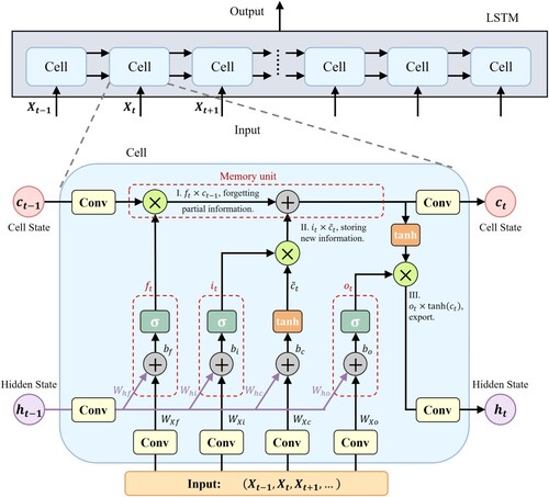
The input gate is represented by $i_t$, the output gate is represented by $o_t$, and the forget gate is represented by $f_t$. The cell state is denoted as $c_t$, the cell output is represented as $h_t$, and the cell input is denoted as $X_t$. The weights for each gate are represented as $W$, and the corresponding bias vectors are represented as $b$. The detailed calculation process for the gates and states of the ConvLSTM unit can be divided into three parts.

Firstly, forget gate ($f_t$) is calculated according to input data ($X_t$) at time $t$ and previous hidden state ($h_{t-1}$), shown in eq. (8(8) $f_t=\sigma (\mathrm{Conv}(W_{\mathrm{Xf}}{X}_t)+\mathrm{Conv}(W_{\mathrm{hf}}{h}_{t-1})+b_f),$(8) ). (8) $f_t=\sigma (\mathrm{Conv}(W_{\mathrm{Xf}}{X}_t)+\mathrm{Conv}(W_{\mathrm{hf}}{h}_{t-1})+b_f),$(8) where $\sigma$ denotes the sigmoid activation function that maps $f_t$ into the range (0, 1).

Next, the input gate ($i_t$) is designed as eq. (9(9) $\begin{array}{rl}{i}_t& =\sigma (\mathrm{Conv}(W_{\mathrm{Xi}}{X}_t)+\mathrm{Conv}(W_{\mathrm{hi}}{h}_{t-1})+b_i),\end{array}$(9) ), and its treatment similar to the forget gate ($f_t$) maintains its range within (0, 1) for filtering purposes. A new candidate cell ($\widetilde{c_t}$) is created as eq. (10(10) $\begin{array}{rl}\widetilde{c_t}& =\tanh (\mathrm{Conv}(W_{\mathrm{Xc}}{X}_t)+\mathrm{Conv}(W_{\mathrm{hc}}{h}_{t-1})+b_c),\end{array}$(10) ), which is the activation of the input data under the current time and the hidden state ($h_{t-1}$). Subsequently, the new cell state ($c_t$) is updated by combining partial stored information from $X_t$ and the old remaining information from the forget processing, as shown in eq. (11(11) $\begin{array}{rl}{c}_t& =f_t\times c_{t-1}+i_t\times \widetilde{c_t},\end{array}$(11) ). (9) $\begin{array}{rl}{i}_t& =\sigma (\mathrm{Conv}(W_{\mathrm{Xi}}{X}_t)+\mathrm{Conv}(W_{\mathrm{hi}}{h}_{t-1})+b_i),\end{array}$(9) (10) $\begin{array}{rl}\widetilde{c_t}& =\tanh (\mathrm{Conv}(W_{\mathrm{Xc}}{X}_t)+\mathrm{Conv}(W_{\mathrm{hc}}{h}_{t-1})+b_c),\end{array}$(10) (11) $\begin{array}{rl}{c}_t& =f_t\times c_{t-1}+i_t\times \widetilde{c_t},\end{array}$(11) where tanh denotes the hyperbolic tangent activation function, which maps the input to the range ( – 1, 1).

Finally, the new hidden state ($h_t$) is obtained through the output gate ($o_t$) and the cell state ($c_t$). The calculation formula is as follows: (12) $\begin{array}{rl}{o}_t& =\sigma (\text{Conv}(W_{\mathrm{Xo}}{X}_t)+\text{Conv}(W_{\mathrm{ho}}{h}_{t-1})+b_o),\end{array}$(12) (13) $\begin{array}{rl}{h}_t& =o_t\times \tanh (c_t),\end{array}$(13) Particularly, as an improved variant of ConvLSTM, the bidirectional ConvLSTM (BiConvLSTM) employed here consists of two layers of ConvLSTM, with one transmitting the spatio-temporal information forwardly and the other performing converse operation (Hanson et al., 2018). Thus, the BiConvLSTM can combine both past and future information, making it potential to better understand the underlying complicated spatio-temporal evolution laws. Figure 9 illustrates the functionality of a BiConvLSTM module consisting of the ConvLSTM cells with two sets of hidden states and cell states.

Figure 9. HDNN framework.

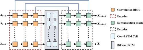
3.1.3. Network structure

Utilising the UConv module for handling large-scale graphs and the ConvLSTM module for extracting spatio-temporal features, this section attempts to construct the complete HDNN model for learning the 2D unsteady FSI flow fields. For the problem of predicting the unsteady flow fields caused by fish movement, given historical data $X_{t-k},\dots ,X_{t-1}$, the goal is to predict the flow field ${\hat{X}}_t$ at time $t$. Given the unstructured spatio-temporal model, there are usually output modes. The first mode is sequence-to-one (S2O) (Liu et al., 2022), which can be described as predicting the data at the next time-step with the input of historical time sequence data, represented as $[X_{t-k},\dots ,X_{t-1}]\stackrel{M}{\to }{\hat{X}}_t$. The second mode is sequence-to-sequence (S2S) (Eivazi et al., 2020), which can be described as predicting the flow fields for the next time sequence with the input of historical time sequence data, represented as $[X_{t-k},\dots ,X_{t-1}]\stackrel{M}{\to }[{\hat{X}}_t,\dots ,{\hat{X}}_{t+k-1}]$. Compared to the S2S approach, the model with S2O may be difficult to capture the temporal relationships of unsteady flow, as it optimises the network only using single time-step output during the backpropagation process, without considering for multi-time coupling. Therefore, this paper chooses S2S as the output mode for the HDNN model.

In this work, the proposed HDNN model follows an encoder-processor-decoder structure, allowing it to effectively learn the intricate spatio-temporal patterns of unsteady FSI flow fields. Specifically, both the encoder and decoder are implemented through the UConv module, focusing on achieving high-dimensional spatial mappings and feature alignment. The encoder-decoder structure of HDNN consists of k encoding parts and k decoding parts. Each encoding part comprises 3 convolutional blocks (orange blocks in Figure 9), and each decoding part comprises 3 deconvolutional blocks (green blocks in Figure 9). Each convolutional or deconvolutional block includes 3 convolutional or deconvolutional layers and max pooling or max unpooling layers, as shown in Figure 5. Additionally, the processor of HDNN is implemented using BiConvLSTM, comprising two parallel ConvLSTM layers in bidirectional propagation, to effectively capture the long-term spatio-temporal dynamics of unsteady flow fields. Specifically, the forward pass generates hidden states ($h^f$) and cell states ($c^f$); conversely, the backward pass generates hidden states ($h^b$) and cell states ($c^b$). These hidden states are aggregated and mapped to the outputs through the decoder as. (14) $\begin{array}{rl}{\hat{X}}_t,\dots ,{\hat{X}}_{t+k-1}& =\text{UConv}([h_{t-k}^f,\dots ,h_{t-1}^f]\\ & +[h_{t-k}^b,\dots ,h_{t-1}^b]),\end{array}$(14)

3.2. Training method

The training process of neural networks is an optimisation procedure guided by the minimisation of the loss function. In this paper, the optimisation process of the hybrid neural network utilises the Adam optimisation algorithm. The choice of loss function is pivotal in the prediction process.

The loss function in the study is represented by the weighted sum of root mean square errors (RMSE) for k output snapshots. (15) $\text{RMS}{\text{E}}_t=\sqrt{\frac{{\sum }_{i=1}^N{({\hat{X}}_t^i-X_t^i)}^2}{N}},$(15) where $t$ is the instantaneous output, $\text{RMS}{\text{E}}_t$ is the RMSE between the transient predicted flow field and the CFD flow field, ${\hat{X}}_t^i$ and $X_t^i$ represent the predicted and numerical simulation values at node i, and N is the number of nodes in the image. (16) $\begin{array}{rl}\mathrm{Loss}& ={\lambda }_1\text{RMS}{\text{E}}_t+{\lambda }_2\text{RMS}{\text{E}}_{t+1}+,\dots ,\\ & +{\lambda }_k\text{RMS}{\text{E}}_{t+k-1},\end{array}$(16) where (${\lambda }_1,{\lambda }_2,\dots ,{\lambda }_k$) represents the weight coefficient of the hybrid loss function for k time series outputs. The values are uniformly set to $\frac{1}{k}$, serving as an average to learn the spatio-temporal relationships among various prediction sequences.

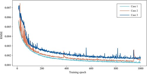
The NVIDIA RTX 4070 GPU and i7-13700 K CPU are utilised for numerical simulations, and the Paddle open-source software library is employed for network training. The learning rate for HDNN training is set to 0.001, and the number of training epochs is set to 1000. Figure 10 illustrates the RMSE reduction for the three datasets with increasing training step. After 600 training steps, the training error converged to below 0.002, indicating the stability of the prediction architecture of HDNN during the training process for the three cases.

Figure 10. Training losses of HDNN for three datasets.

3.3. Prediction method

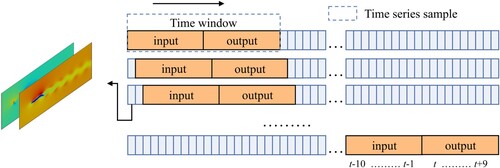
Inspired by the transient dynamic prediction scenario mentioned by Liu et al. (2022), an iterative prediction strategy is adopted for the sequence flow field prediction process. This method involves utilising the outputs of the transient prediction process as inputs for successive iterations, as depicted in Figure 11. As mentioned in Section 2.2.2, k is set to 10, implying the use of 10 consecutive time-steps CFD results to predict the future changes for an entire cycle (with 60 consecutive time-steps in one cycle). In engineering applications, more emphasis is placed on the model’s long-term predictive capability, i.e. multi-step rolling predicting subsequent results through the initial time sequence of the test set.

Figure 11. Method of multi-step rolling prediction.

3.4. Evaluation metric

In order to quantitatively evaluate the quality of flow field snapshot prediction, the well-known peak signal-to-noise ratio (PSNR) and structural similarity index (SSIM) standards from the field of image monitoring are adopted (Zhou et al., 2004). These two metrics are also widely used in the evaluation of flow field reconstruction models (Hao et al., 2023; Xie et al., 2023). For the predicted flow field ${\hat{X}}_t$ at time $t$ and the numerically simulated flow field $X_t$, the corresponding PSNR and SSIM are defined as follows: (17) $\begin{array}{rl}& \text{PSNR}=20\times {\log }_{10}\left(\frac{\mathrm{MA}{X}_I}{\text{mean}({({\hat{X}}^t-X^t)}^2)}\right),\end{array}$(17) (18) $\begin{array}{rl}& \text{SSIM}\\ & =\frac{(2\mu ({\hat{X}}_t)\mu (X_t)+c_1)(2\text{cov}({\hat{X}}_t,X_t)+c_2)}{(\mu {({\hat{X}}_t)}^2+\mu {(X_t)}^2+c_1)(\nu {({\hat{X}}_t)}^2+\nu {({\hat{X}}_t)}^2+c_2)},\end{array}$(18) where $\mathrm{MA}{X}_I$ = 1 is the maximum pixel value of an image since ${\hat{X}}_t$ and $X_t$ are float tensors; $\mu$ and $\nu$ are the mean and variance of an image; cov represents the covariance between two images; and finally, $c_1$ =  1 × 10⁻⁴ and $c_2$ = 9 × 10⁻⁴ are constants used to maintain stability.

The PSNR is a measurement standard for evaluating image quality, and it is defined as the ratio of energy of the peak signal to the average energy of noise, usually expressed by taking log into decibels (dB). A larger PSNR value implies a less distorted image. Differently, the SSIM could quantify the structural similarity between two images by using the mean, variance and covariance to estimate brightness, contrast, and structural similarity, respectively. The SSIM value falls within (0, 1), and the similarity between two images increases with SSIM.

4. Results and discussions

This section tests the proposed method on flow field datasets under three cases, assessing the predictive capability, generalisation performance, and computational efficiency of HDNN. Simultaneously, an ablation study is conducted to compare the prediction results of different variants, investigating the roles of the modules within the model.

4.1. Evaluation of model forecasting

This study designs three cases to test the ability of the proposed model: (1) Case 1 and Case 2 are designed to evaluate the performance of the neural network in predicting unsteady flows caused by fish movement with different tail-beat frequencies, revealing whether the neural network can capture the spatio-temporal characteristics of unsteady flows under different conditions. Case 1 involves the flow under the slow tail-beat condition of fish at $f$ = 0.4 Hz, while Case 2 involves the flow under the fast tail-beat condition of fish at $f$ = 3 Hz. They exhibit different physical characteristics. Whether the same neural network structure can be applied to two different flows is a criterion for testing the applicability of the HDNN. (2) Case 3 is used to test the generalisation ability of the neural network, i.e. whether HDNN can be used to predict flows not used for training. In this experiment, the flow data in Case 3–1 to Case 3–6 are used as the dataset for training the neural network to capture the underlying dynamics, while the dataset for testing included extrapolation states (Case 3-7) and interpolation states (Case 3-8).

Table 2 reports the average and standard deviation of PSNR and SSIM for the proposed HDNN model for 60 time-step rolling predictions on the whole sequences of four test sets. It is observed that the PSNR values of two physical quantities are larger than 34 dB, with corresponding SSIM values exceeding 0.9. This suggests that the predicted flow fields closely align with the simulated flow fields, indicating effective learning of the complex spatio-temporal evolution laws governing flow velocity transfer. As for the extrapolation Cases 3-7, its performance is slightly worse than the interpolation Case 3-8, as evidenced by the comparatively smaller PSNR and SSIM values in Table 3. This observation is rationalised by the fact that the operating conditions of Case 3–7 lie outside the training range, necessitating extrapolation. But even for the challenging Case 3-7, its predictions achieve good PSNR and SSIM values, demonstrating the strong generalisation capabilities of the HDNN.

Table 2. The average and standard deviation of PSNR and SSIM values of the proposed HDNN for 60 time-steps rolling predictions on the whole sequences of four test sets.

Case	Sample size	Metric	$V_x$	$V_y$
Case 1 (test set)	180	PSNR	39.449 ± 0.848	39.994 ± 0.460
		SSIM	0.978 ± 0.004	0.958 ± 0.004
Case 2 (test set)	180	PSNR	40.561 ± 1.425	44.196 ± 0.734
		SSIM	0.976 ± 0.006	0.978 ± 0.003
Case 3–7	300	PSNR	37.653 ± 0.685	34.396 ± 0.179
		SSIM	0.966 ± 0.006	0.915 ± 0.005
Case 3–8	300	PSNR	42.528 ± 1.286	42.560 ± 0.633
		SSIM	0.984 ± 0.003	0.970 ± 0.003

Table 3. Comparison of computational time required by the Fluent unsteady simulator and the data-driven HDNN model for the effect of fish swimming on flow field.

		Predicting (s)
Cases	HDNN training (s)	CFD	HDNN	Speedup
Case 1	53 725	20 384	148.695	137 times
Case 2	51 228	39 017	115.379	338 times
Case 3	56 799	19 818	133.994	148 times

More detailedly, Figures 12–15 show the comparison between the predictions of the HDNN after a full cycle (60 time-steps) and the results of CFD calculations for four different test sets. Through this comparison, it is evident that the predicted flow fields align well with the CFD simulated flow fields in all cases. The predicted flow field distribution, fish body shape, and the movement of wake closely match the numerical computation results, showing a basic synchronisation in temporal changes. This demonstrates the ability of HDNN to predict and capture the complete spatio-temporal evolution of the FSI. Additionally, the errors in the transient flow field predictions are mainly concentrated at the tail and wake, where there is a relative noticeable area of high-value error. The primary reason is that the location of wake and tail exits sharp gradient of flow field change, which is very difficult to capture characteristics.

Figure 12. Comparisons of instantaneous flow fields after 60 time-steps between the model predictions and CFD results for Case 1 ($f$ = 0.4 Hz): CFD results for (a) $V_x$ and (b) $V_y$; network predictions for (c) $V_x$ and (d) $V_y$; and absolute prediction error for (e) $V_x$ and (f) $V_y$.

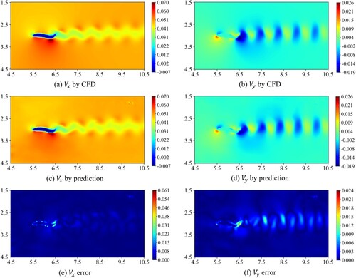
Figure 13. Comparisons of instantaneous flow fields after 60 time-steps between the model predictions and CFD results for Case 2 ($f$ = 3 Hz): CFD results for (a) $V_x$ and (b) $V_y$; network predictions for (c) $V_x$ and (d) $V_y$; and absolute prediction error for (e) $V_x$ and (f) $V_y$.

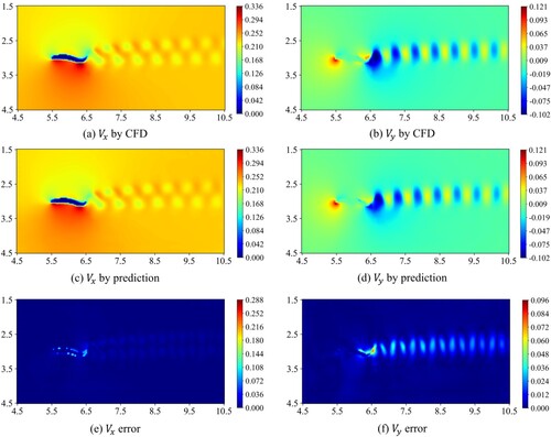
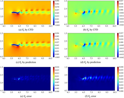
Figure 14. Comparisons of instantaneous flow fields after 60 time-steps between the model predictions and CFD results for Case 3–7 ($f$ = 1.1 Hz): CFD results for (a) $V_x$ and (b) $V_y$; network predictions for (c) $V_x$ and (d) $V_y$; and absolute prediction error for (e) $V_x$ and (f) $V_y$.

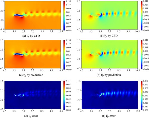
Figure 15. Comparisons of instantaneous flow fields after 60 time-steps between the model predictions and CFD results for Case 3–8 ($f$ = 0.65 Hz): CFD results for (a) $V_x$ and (b) $V_y$; network predictions for (c) $V_x$ and (d) $V_y$; and absolute prediction error for (e) $V_x$ and (f) $V_y$.

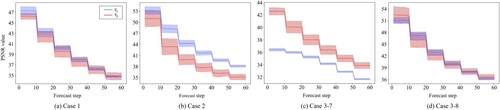
Finally, Figure 16 shows the prediction of two physical quantities of HDNN in terms of PSNR for 60 time-steps in Case 1, Case 2, Case 3-7, and Case 3-8. It is observed that the prediction quality of the four test sets decrease with the forecast steps. However, the PSNR values at the 60th time-step for all four test sets remain above 30 dB, demonstrating that the proposed HDNN model can effectively predict the long-term evolution of the FSI flow field. Additionally, an interesting phenomenon is that the average of PSNR values for the HDNN model shows a ‘step-like’ decrease, that is, after each time sequence size (k = 10) rolling forecast, PSNR will suddenly drop. This is because the rolling prediction method causes errors to accumulate as the forecast steps increase, while the S2S output method can obtain the results for the future k steps for each prediction, effectively reducing the accumulation of errors within each k step. Therefore, in the application of the proposed HDNN multi-step rolling prediction, it is possible to further improve the model prediction accuracy by appropriately increasing the size of k, given the available computational resources.

Figure 16. Average and standard deviation of PSNR values of the proposed HDNN predictions for $V_x$ and $V_y$ at 60 time-steps of (a) Case 1, (b) Case 2, (c) Case 3–7 and (d) Case 3-8. The shaded area depicts the average ± the standard deviation over the whole test sequence.

4.2. Ablation study

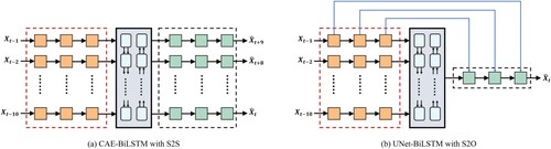
The results indicate that the proposed HDNN model has demonstrated significant performance in predicting the three cases. The UConv module plays a crucial role in this model, as it effectively extracts underlying spatial patterns on one hand, and captures the underlying temporal connections through the S2S corresponding multi-decoding structure on the other. To investigate the effectiveness of the UConv module construction, this section conducts an ablation study using the dataset of Case 1 as an example, comparing the reconstruction effects on velocity magnitude. As shown in Figure 17, this study considers two additional variants for comparative experiments. The first variant involves removing the U-shaped connection on the basis of the proposed model, denoted as CAE-BiLSTM with S2S. The second variant uses the S2O corresponding decoding structure, denoted as UNet-BiLSTM with S2O. The variant model CAE-BiLSTM with S2S is a commonly used unsteady flow field reconstruction structure.

Figure 17. Convolutional neural network variants investigated in this work. (a) CAE-BiLSTM with S2S; (b) UNet-BiLSTM with S2O.

Effectiveness of U-shaped connection. Figure 18 illustrates the velocity magnitude prediction over 60 time-steps in Case 1 for the three models, as measured by PSNR. It is evident that, compared to CAE-BiLSTM with S2S, the HDNN model with the introduction of the U-shaped connection exhibits better performance in forecasting over 60 time-steps. The average of PSNR values at the 60th time-step increased by 3.322. More specifically, comparing Figure 19 (a), (b), and (e), it can be found that the CAE-BiLSTM with S2S starts to produce noise in the predicted flow field at n = 24, resulting in non-smooth reconstructed images, which worsens as the prediction progresses. This is due to the convolution process of CAE causing the loss of flow field information. Therefore, by introducing the U-shaped connection, the generation of noise is successfully avoided (Figure 19 (d)), demonstrating the effectiveness of the U-shaped connection in capturing long-term relationships. The encoding layer obtains more accurate feature information, leading to more precise segmentation results after upsampling.

Figure 18. Average and standard deviation of PSNR values of the proposed HDNN and its architecture variants predictions for velocity magnitude at 60 time-steps of Case 1. The shaded area depicts the average ± the standard deviation over the whole test sequence.

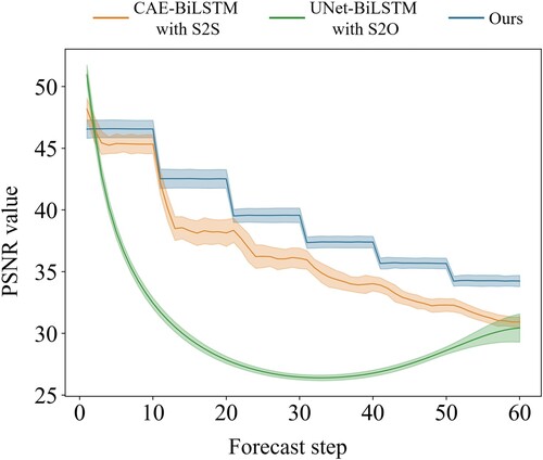
Figure 19. Comparisons of the velocity magnitude flow fields among the CAE-BiLSTM with S2S, UNet-BiLSTM with S2O and HDNN. (a) the CFD flow fields; (b) the predicted flow fields obtained by CAE-BiLSTM with S2S; (c) the predicted flow fields obtained by UNet-BiLSTM with S2O; (d) the predicted flow fields obtained by HDNN; (e) the absolute error contours of prediction, where the first line is obtained by CAE-BiLSTM with S2S, and the second line is obtained by UNet-BiLSTM with S2O, and the third line is obtained by HDNN.

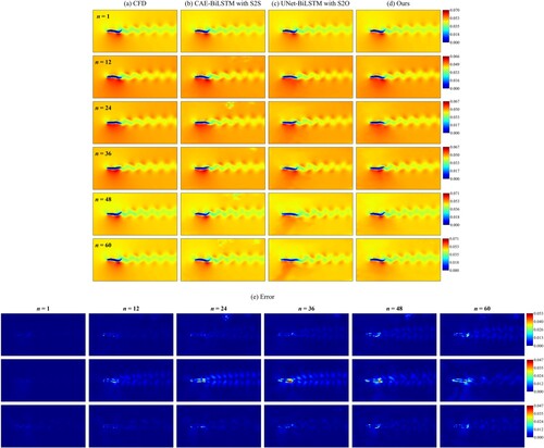
Effectiveness of S2S. The UNet-BiLSTM model with S2S is tested to evaluate its performance. From Figure 18, it can be observed that the model’s performance is further improved compared to UNet-BiLSTM with S2O. With the use of the S2S corresponding to the multi-decoding structure, the average of PSNR values at the 60th time-step increased by 3.803. Additionally, comparing Figure 19 (a), (c), and (e), it can be observed that UNet-BiLSTM with S2O starts to gradually deviate from the fish body shape and shock wave position of the reconstructed flow field from CFD at n = 24, showing that the simulated fish tail-beat speed and wake propagation speed are faster than the actual situation, and this phenomenon worsens as the prediction progresses. However, after introducing the multi-decoding structure with S2S, the model’s temporal synchronicity is effectively improved (Figure 19 (b)), indicating that the backpropagation based on the multi-decoding structure with S2S can enable the model to capture more detailed temporal information, thereby improving the results of multi-step rolling prediction.

4.3. Efficiency of model forecasting

The previously proposed HDNN model provides accurate and rapid spatio-temporal prediction in 2D unsteady and unstructured FSI flow fields. Therefore, this section investigates the predictive efficiency of the model. Table 3 reports the time required for training and prediction using both the Fluent unsteady simulator and the data-driven HDNN model. The Fluent simulation setup is equipped with a 13th Gen Intel(R) Core(TM) i7-13700 K 16-core processor, while the HDNN model setup is equipped with NVIDIA RTX 4070 GPU computing.

It has been observed that the training time of the HDNN model, trained on a large dataset collected from simulation cases, exceeds the simulation time of a single case in Fluent. However, once the model is trained, it can provide rapid predictions, resulting in a two orders of magnitude speedup, as shown in Table 3. Additionally, as the simulation time-step in CFD is inversely proportional to the tail-beat frequency, the computational time of CFD increases with the increase in the tail-beat frequency of the simulation condition, whereas the time taken by the HDNN model is not affected by the tail-beat frequency. Therefore, the HDNN model can significantly reduce the prediction time, achieve real-time prediction of unsteady FSI flow fields, and enhance task efficiency and quality.

5. Conclusion

Flow field reconstruction is of great significance for studying the underlying principles of fish swimming behaviour and for the developing fish passage facilities. This paper aims to develop a data-driven spatio-temporal modelling and prediction method for unsteady flow fields around fish, in order to alleviate the need for extensive time-consuming numerical simulations or experiments. In particular, this study proposes a data-driven deep spatio-temporal sequence model, HDNN, which establishes an intelligent framework based on DL for modelling and efficiently predicting 2D unsteady flow fields caused by fish movement. In this model, the (1) UConv module is adopted to effectively learn large-scale unstructured flow fields, and (2) the BiConvLSTM module is established to efficiently extract spatio-temporal features of unstructured data. Specifically, this model adopts a S2S input-output format to mitigate error accumulation during multi-step rolling predictions.

In order to demonstrate the effectiveness and robustness of the proposed method, three different cases are used for training and testing. Trained HDNN is tested by predicting future flow fields. Based on this, the following conclusions can be drawn. Firstly, the proposed HDNN successfully learned the spatio-temporal evolution of FSI flow fields under different tail-beat frequencies, enabling accurate multi-step predictions. The predicted flow fields by HDNN not only highly match the simulation results but are also several hundred times faster than traditional numerical simulations. Secondly, HDNN is able to perform reasonable spatio-temporal extrapolation based on the learned flow field evolution patterns, even for long-term predictions, demonstrating strong generalisation capabilities. Finally, through ablation experiments, this study demonstrates that the U-shaped connection and the S2S input-output format can effectively improve the prediction performance.

As far as the authors know, this is the first attempt to apply DL to the modelling and predicting of the spatio-temporal evolution of flow fields influenced by fish movement. Currently, the HDNN model is used to predict flow under different behaviour conditions. Due to its flexible data-driven framework, it can certainly be trained on more data collected from various operating conditions to enhance the model capability. Furthermore, the current study reconstructs the flow situation in the Lagrangian framework, and future improvements may involve exploring how to embed the proposed model into more complex Eulerian flow field environments.

Disclosure statement

No potential conflict of interest was reported by the author(s).

Data availability statement

Data available on request from the authors.

Additional information

Funding

This work was supported by National Key Research and Development Program of China: [Grant Number No. 2022YFC3204202]; Basic Research Fund of China Institute of Water Resources and Hydropower Research: [Grant Number No. HY110145B0012023]; the Basic Research Fund of China Institute of Water Resources and Hydropower Research: [Grant Number No. HY110145B0012023].

References

- Cai, G., Zhang, B., Liu, L., Weng, H., Wang, W., & He, B. (2022). Fast vacuum plume prediction using a convolutional neural networks-based direct simulation Monte Carlo method. Aerospace Science and Technology, 129, 107852. https://doi.org/10.1016/j.ast.2022.107852
- Chen, S. Y., Fei, Y. J., Chen, Y. C., Chi, K. J., & Yang, J. T. (2016). The swimming patterns and energy-saving mechanism revealed from three fish in a school. Ocean Engineering, 122, 22–31. https://doi.org/10.1016/j.oceaneng.2016.06.018
- Curatolo, M., & Teresi, L. (2015). The virtual aquarium: Simulations of fish swimming. The Proceedings of the 2015 COMSOL Conference.
- De Bie, J., Manes, C., & Kemp, P. S. (2020). Collective behaviour of fish in the presence and absence of flow. Animal Behaviour, 167, 151–159. https://doi.org/10.1016/j.anbehav.2020.07.003
- Eivazi, H., Veisi, H., Naderi, M. H., & Esfahanian, V. (2020). Deep neural networks for nonlinear model order reduction of unsteady flows. Physics of Fluids, 32(10), 105104. https://doi.org/10.1063/5.0020526
- Fukagata, K., Fukami, K., & Taira, K. (2019). Super-resolution reconstruction of turbulent flows with machine learning. Journal of Fluid Mechanics, 870, 106–120. https://doi.org/10.1017/jfm.2019.238
- Guo, X., Li, W., & Iorio, F. (2016). Convolutional neural networks for steady flow approximation. Proceedings of the 22nd ACM SIGKDD International Conference on Knowledge Discovery and Data Mining (pp. 481–490).
- Han, R., Wang, Y., Zhang, Y., & Chen, G. (2019). A novel spatial-temporal prediction method for unsteady wake flows based on hybrid deep neural network. Physics of Fluids, 31(12), 127101. https://doi.org/10.1063/1.5127247
- Hanson, A., Pnvr, K., Krishnagopal, S., & Davis, L. (2018). Bidirectional convolutional LSTM for the detection of violence in videos. Proceedings of the european conference on computer vision (ECCV) workshops (pp. 285–295).
- Hao, Y., Xie, X., Zhao, P., Wang, X., Ding, J., Xie, R., & Liu, H. (2023). Forecasting three-dimensional unsteady multi-phase flow fields in the coal-supercritical water fluidized bed reactor via graph neural networks. Energy, 282, 128880. https://doi.org/10.1016/j.energy.2023.128880
- Khalid, M. S. U., Akhtar, I., Imtiaz, H., Dong, H., & Wu, B. (2018). On the hydrodynamics and nonlinear interaction between fish in tandem configuration. Ocean Engineering, 157, 108–120. https://doi.org/10.1016/j.oceaneng.2018.03.049
- Kong, L., Wei, W., & Yan, Q. (2018). Application of flow field decomposition and reconstruction in studying and modeling the characteristics of a cartridge valve. Engineering Applications of Computational Fluid Mechanics, 12(1), 385–396. https://doi.org/10.1080/19942060.2018.1438925
- Li, Y., Pan, Z., & Xia, J. (2022a). Computational analysis on propulsive characteristic of flexible foil undergoing travelling wave motion in ground effect. Ocean Engineering, 253, 111300. https://doi.org/10.1016/j.oceaneng.2022.111300
- Li, Z., Xia, D., Cao, J., Chen, W., & Wang, X. (2022b). Hydrodynamics study of dolphin's self-yaw motion realized by spanwise flexibility of caudal fin. Journal of Ocean Engineering and Science, 7(3), 213–224. https://doi.org/10.1016/j.joes.2021.07.011
- Li, Z., Xia, D., Zhou, X., Cao, J., Chen, W., & Wang, X. (2022c). The hydrodynamics of self-rolling locomotion driven by the flexible pectoral fins of 3-D bionic dolphin. Journal of Ocean Engineering and Science, 7(1), 29–40. https://doi.org/10.1016/j.joes.2021.04.006
- Li, C., Yuan, P., Liu, Y., Tan, J., Si, X., Wang, S., & Cao, Y. (2023). Fast flow field prediction of hydrofoils based on deep learning. Ocean Engineering, 281, 114743. https://doi.org/10.1016/j.oceaneng.2023.114743
- Liao, J. C., Beal, D. N., Lauder, G. V., & Triantafyllou, M. S. (2003). Fish exploiting vortices decrease muscle activity. Science, 302(5650), 1566–1569. https://doi.org/10.1126/science.1088295
- Liu, Z., Han, R., Zhang, M., Zhang, Y., Zhou, H., Wang, G., & Chen, G. (2022). An enhanced hybrid deep neural network reduced-order model for transonic buffet flow prediction. Aerospace Science and Technology, 126, 107636. https://doi.org/10.1016/j.ast.2022.107636
- Liu, H., Lin, J., Wang, D., Huang, J., Jiang, H., Zhang, D., Peng, Q., & Yang, J. (2023a). Experimental study of the behavioral response of fish to changes in hydrodynamic indicators in a near-natural environment. Ecological Indicators, 154, 110813. https://doi.org/10.1016/j.ecolind.2023.110813
- Liu, H., Zhou, Y., Ren, X., Liu, S., Liu, H., & Li, M. (2023b). Numerical modeling and application of the effects of fish movement on flow field in recirculating aquaculture system. Ocean Engineering, 285, 115432. https://doi.org/10.1016/j.oceaneng.2023.115432
- Meng, F., Wang, J., Chen, Z., Qiao, F., & Yang, D. (2023). Shaping the concentration of petroleum hydrocarbon pollution in soil: A machine learning and resistivity-based prediction method. Journal of Environmental Management, 345, 118817. https://doi.org/10.1016/j.jenvman.2023.118817
- Palmer, M., & Ruhi, A. (2019). Linkages between flow regime, biota, and ecosystem processes: Implications for river restoration. Science, 365(6459), eaaw2087. https://doi.org/10.1126/science.aaw2087
- Ronneberger, O., Fischer, P., & Brox, T. (2015). U-Net: Convolutional networks for biomedical image segmentation. Medical Image Computing and Computer-Assisted Intervention – MICCAI 2015 (pp. 234–241).
- Rui, E. Z., Chen, Z. W., Ni, Y. Q., Yuan, L., & Zeng, G. Z. (2023). Reconstruction of 3D flow field around a building model in wind tunnel: A novel physics-informed neural network framework adopting dynamic prioritization self-adaptive loss balance strategy. Engineering Applications of Computational Fluid Mechanics, 17(1), 2238849. https://doi.org/10.1080/19942060.2023.2238849
- Shi, X., Chen, Z., Wang, H., Yeung, D. Y., Wong, W. K., & Woo, W. C. (2015). Convolutional LSTM Network: A machine learning approach for precipitation nowcasting. Proceedings of the 28th International Conference on Neural Information Processing Systems – Volume 1 (pp. 802–810).
- Silva, A. T., Bærum, K. M., Hedger, R. D., Baktoft, H., Fjeldstad, H. P., Gjelland, KØ, Økland, F., & Forseth, T. (2020). The effects of hydrodynamics on the three-dimensional downstream migratory movement of Atlantic salmon. Science of The Total Environment, 705, 135773. https://doi.org/10.1016/j.scitotenv.2019.135773
- Tang, M. F., Xu, T. J., Dong, G. H., Zhao, Y. P., & Guo, W. J. (2017). Numerical simulation of the effects of fish behavior on flow dynamics around net cage. Applied Ocean Research, 64, 258–280. https://doi.org/10.1016/j.apor.2017.03.006
- Videler, J. J., & Hess, F. (1984). Fast continuous swimming of two pelagic predators, Saithe (Pollachius virens) and Mackerel (Scomber scombrus): A kinematic analysis. Journal of Experimental Biology, 109(1), 209–228. https://doi.org/10.1242/jeb.109.1.209
- Wang, J., Qie, Z., Li, G., Ran, Y., & Wu, X. (2023). An efficient fish migration modeling method integrating the random forest and Eulerian–Lagrangian–agent method for vertical slot fishways. Ecological Engineering, 195, 107067. https://doi.org/10.1016/j.ecoleng.2023.107067
- Wang, L., & Wu, C. (2010). An adaptive version of ghost-cell immersed boundary method for incompressible flows with complex stationary and moving boundaries. Science China Physics, Mechanics and Astronomy, 53(5), 923–932. https://doi.org/10.1007/s11433-010-0185-z
- Wei, C., Hu, Q., Zhang, T., & Zeng, Y. (2022). Passive hydrodynamic interactions in minimal fish schools. Ocean Engineering, 247, 110574. https://doi.org/10.1016/j.oceaneng.2022.110574
- Wohl, E., Lane, S. N., & Wilcox, A. C. (2015). The science and practice of river restoration. Water Resources Research, 51(8), 5974–5997. https://doi.org/10.1002/2014WR016874
- Xie, X., Wang, X., Zhao, P., Hao, Y., Xie, R., & Liu, H. (2023). Learning time-aware multi-phase flow fields in coal-supercritical water fluidized bed reactor with deep learning. Energy, 263, 125907. https://doi.org/10.1016/j.energy.2022.125907
- Zhao, Z., & Shi, Q. (2023). Hydrodynamic interactions coordinate the swimming of two self-propelled fish-like swimmers. Ocean Engineering, 284, 115263. https://doi.org/10.1016/j.oceaneng.2023.115263
- Zhong, H., Wei, Z., Man, Y., Pan, S., Zhang, J., Niu, B., Yu, X., Ouyang, Y., & Xiong, Q. (2023). Prediction of instantaneous yield of bio-oil in fluidized biomass pyrolysis using long short-term memory network based on computational fluid dynamics data. Journal of Cleaner Production, 391, 136192. https://doi.org/10.1016/j.jclepro.2023.136192
- Zhou, W., Bovik, A. C., Sheikh, H. R., & Simoncelli, E. P. (2004). Image quality assessment: From error visibility to structural similarity. IEEE Transactions on Image Processing, 13(4), 600–612. https://doi.org/10.1109/TIP.2003.819861