High spatial variability of gas transfer velocity in streams revealed by turbulence measurements

ABSTRACT

Streams are major sources of carbon dioxide (CO₂) and methane (CH₄) to the atmosphere, but current large-scale estimates are associated with high uncertainties because knowledge concerning the spatiotemporal control on stream emissions is limited. One of the largest uncertainties derives from the choice of gas transfer velocity (k₆₀₀), which describes the physical efficiency of gas exchange across the water–atmosphere interface. This study therefore explored the variability in k₆₀₀ and subsequent CO₂ and CH₄ emission rates within and across streams of different stream order (SO). We conducted, for the first time in streams, direct turbulence measurements using an acoustic Doppler velocimeter (ADV) to determine the spatial variability in k₆₀₀ across a variety of scales with a consistent methodology. The results show high spatial variability in k₆₀₀ and corresponding CO₂ and CH₄ emissions at small spatial scales, both within stream reaches and across SO, especially during high discharge. The k₆₀₀ was positively related to current velocity and Reynolds number. By contrast, no clear relationship was found between k₆₀₀ and specific stream characteristics such as width and depth, which are parameters often used in empirical models of k₆₀₀. Improved understanding of the small-scale variability in the physical properties along streams, especially during high discharge, is therefore an important step to reduce the uncertainty in existing gas transfer models and emissions for stream systems. The ADV method was a useful tool for revealing spatial variability in this work, but it needs further development. We recommend that future studies conduct measurements over shorter time periods (e.g., 10–15  min instead of 40  min) and at more sites across the reach of interest, and thereby derive more reliable mean-reach k₆₀₀ as well as more information about controls on the spatial variability in k₆₀₀.

KEYWORDS:

• biogeochemistry
• gas exchange
• spatial variability
• streams

Introduction

Streams and rivers are major emitters of carbon dioxide (CO₂) to the atmosphere, estimated to emit 1.8 PgC yr⁻¹, equal to ∼85% of the total inland water emissions of CO₂ (Raymond et al. 2013) and 0.03 PgC yr⁻¹ of methane (CH₄; Stanley et al. 2016). A disproportionately high contribution of these stream and river emissions is suggested to derive from low-order streams (Raymond et al. 2013). Despite this major importance, knowledge concerning controls on stream emissions in space and time is limited. Stream emission scaling requires in principal 3 components: the concentration gradient between water and atmosphere for the gas of interest, the gas transfer velocity describing the physical efficiency for gas exchange across the air–water interface (k), and the areal extent of stream surfaces. Each of the 3 components has its own spatiotemporal dynamics, which must be resolved to produce realistic emission estimates. One of the most challenging tasks when scaling stream emissions to larger landscape units is the choice of appropriate k values. The parameter k is essentially controlled by the physical properties of the stream channel and the water flow, and therefore its measurement is challenging because of the often highly heterogeneous stream geomorphology in combination with a varying discharge over time. Hence, data on stream k are scarce, and models for scaling are rare and possibly site-specific.

Existing parameterizations of k for streams are often based on physical stream properties including stream slope, water velocity, and stream depth (Wallin et al. 2011, Raymond et al. 2012, Natchimuthu et al. 2017); however, the physical drivers of k are suggested to be different depending on system sizes. While wind drag can play a large role in controlling k for higher-order rivers and estuaries, physical properties of the stream channel are the primary control of k in streams of lower stream order (SO; Alin et al. 2011, Wallin et al. 2011). For example, small streams are often shallow, and bottom stress creates turbulence, thus enhancing gas exchange at the air–water interface. Several large-scale studies have also concluded that k decreases with increasing stream and river size (i.e., SO; Wallin et al. 2011, Striegl et al. 2012, Raymond et al. 2013). For example, Raymond et al. (2013) globally modeled mean k values per SO ranging from 10.4  m d⁻¹ in first-order streams to 3.0  m d⁻¹ in 10th-order streams. Similarly, Wallin et al. (2018) estimated the mean k for the stream network of Sweden (SO1–4) ranging from 9.9  m d⁻¹ in first-order streams to 8.8  m d⁻¹ in fourth-order streams.

Quantification of k in streams has mostly been done using gas tracer studies (Hope et al. 2001, Öquist et al. 2009, Natchimuthu et al. 2017) or by inferring k from direct gas flux measurement with floating chambers (Crawford et al. 2013, Campeau et al. 2014). Both these methods have their limitations, however, and are not suitable for all types of stream channels and discharge conditions. These limitations have probably resulted in selection bias toward sites with characteristics suitable for the respective method. For low-order streams, the use of a volatile gas tracer has been the main approach for estimating k (Genereux and Hemond 1990, Wallin et al. 2011, Billett and Harvey 2013). This method has the advantage of integrating k over a stream reach that can be highly heterogeneous in terms of channel morphology and flow characteristics. Although gas tracer injection studies have also been performed on large rivers (Clark et al. 1994, Cook et al. 2006), the size of the system makes the studies labor and time demanding. The gas tracer method is also more challenging in large and deep rivers or in slowly flowing streams because the tracer gas needs to be homogeneously mixed and representatively sampled within the water column (Clark et al. 1994).

Regarding floating chambers, their efficacy on running waters is debatable. A study by Lorke et al. (2015) recently showed that anchored floating chambers, which often have been used in stream studies, disturb the in-stream turbulence and in turn enhance k estimates, something not seen when using drifting chambers. Drifting chambers, however, can be problematic, or even impossible, in fast flowing, shallow, narrow stream reaches with heterogeneous geomorphology that restricts the free drift of the chamber. The drifting chamber technique may therefore be best suited for larger and deeper streams and rivers where the physical interference of the chambers on the turbulence regime in the surface water may be reduced because the water surface is more homogeneous, although this suitability has been questioned as well (Raymond and Cole 2001). Hence, none of the current methods is applicable across all the different types of running waters.

Because water-side turbulence is the main driver of k (Jähne and Haußecker 1998), direct measurements of turbulence may help us better understand how stream emissions are controlled in time and space. The advantage of direct turbulence measurements to derive k for soluble gases is that they are solely based on the physical properties of water flow, regardless of flux or chemical properties of different gases; hence, this method might be more appropriate for estimating transport across aquatic interfaces (Lorke and Peeters 2006). Applying measurements of the dissipation of turbulent kinetic energy (ε) with an acoustic Doppler velocimeter (ADV) and relating ε to k is a method previously applied on lakes (Vachon et al. 2010), rivers (Zappa et al. 2007), coastal seas (Zappa et al. 2007, Gålfalk et al. 2013), and on coral reefs and estuaries (Tokoro et al. 2008) but to our knowledge has never been applied on low-order streams. The method requires in principle a single instrument (the ADV) and may thus be more applicable across different SOs, discharge rates, and channel morphologies than traditional methods to estimate gas transfer in streams.

Here we studied spatial patterns in gas transfer velocities and emissions in low-order streams using an ADV-based approach to derive comparable information from one methodology for a variety of stream characteristics. More specifically, we measured ε and related it to k using previously published relationships. The measurements were taken within a low-order (SO1–4) boreal catchment in mid-Sweden to investigate the variability in stream k within single stream reaches and across stream orders, discharge regimes, and channel morphologies.

Methods

Site description

This study was conducted in an ∼80 km² fourth-order catchment in south-central Sweden (Fig. 1; 59.803279°N, 15.167283°E). The catchment consists of 84.3% forest; 10% wetlands, marshes, fens and bogs; 5.1% lakes; 0.5% agriculture; and 0.06% habitation. Annual average temperature and precipitation at the nearest meteorological station (Kloten A ∼4 km east of site SO1; Swedish Meteorological and Hydrological Institute [SMHI]; www.smhi.se) were 4.7 °C and 780 mm, respectively, during 2010–2015. Mean (modeled) discharge at the farthest downstream site (SO4) was 1.05 m³ s⁻¹ during 1981–2010 (SMHI). Hydrological flowpaths and catchment delineation were determined based on a 2  m resolution digital elevation model (GSD-DEM grid 2+) and with land-use data derived from the GSD-Overview Map (both from the Swedish Land Survey). Analyses were made using the Hydrological Extension tool in ESRI ArcGIS.

Figure 1. Location of sampling sites and corresponding watershed areas in Sweden.

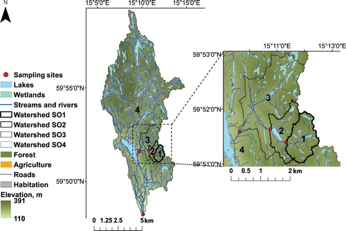
The sampled sites were distributed along a hydrological chain of streams and lakes with streams ranging from SO1 to SO4 (Fig. 1). SO1 is located just upstream of a small lake (0.07 km²) and drains a 1.2 km² catchment, mainly covered by coniferous forest (Supplemental Table S1). SO2 is located just downstream of the outlet of the same lake and drains another 1 km² (total 2.2 km²) of wetlands and coniferous forest. Farther downstream, SO3 is located upstream of a larger lake (1.3 km²) and drains 6.1 km². SO4 is situated in a small village farther downstream, draining 80.1 km². For further information of the area see Einarsdottir et al. (2017), Chmiel et al. (2016), and Denfeld et al. (2015).

Stream discharge (Q) was measured for SO1–3 at each sampling occasion by the salt dilution method (Day 1976). For SO4, water velocity was measured with a flow meter (Höntzsch Instruments, Germany) in horizontal and vertical across-reach transects. The average transect water velocity was multiplied by the cross-section area to obtain an average Q for the stream reach. Water temperature, electrical conductivity, and dissolved oxygen were measured in situ with an HQ40d Portable Multiparameter Meter (HACH), and pH was measured in the lab from water samples on a Metrohm 744 pH meter.

The eddy cell model and ADV-based dissipation rate measurements

We used an ADV (Vector, Nortek, Norway) to measure the 3-dimensional (3D) water velocity (the horizontal components in the along-flow and cross-flow directions u and v, respectively, and the vertical component w). We calculated k₆₀₀ (m s⁻¹, but in the text reported in units of cm h⁻¹) using the eddy cell model (Lamont and Scott 1970; referred to as ADV-k), which assumes that the smallest turbulent eddies in the energy-dissipating range are most important in transporting solutes toward the surface:(1) where is the constant of proportionality, here set to 0.43, which is equal to, or close to, previous findings across multiple settings including coastal ocean, lakes, rivers, and lab-based tanks (Dickey et al. 1984, Zappa et al. 2007, Vachon et al. 2010), is the dimensionless temperature-dependent Schmidt number (Wanninkhof 2014), is the kinematic molecular viscosity of water (m² s⁻¹), and the dissipation rate of turbulent kinetic energy (m² s⁻³). The Schmidt exponent varies depending on the characteristics of the water surface and was here set to one-half according to Jähne et al. (1987) and Wanninkhof (1992). Variable was calculated from the inertial subrange in the power spectrum of the current velocities of the u component (measured by the ADV) according to Kolmogorov’s law:(2) where is the wave number spectrum of the current velocity (m³ s⁻²), is the dimensionless Kolmogorov’s constant (0.52 for the u component; Högström 1996), and is the wave number (m⁻¹). Because we took measurements by maintaining the ADV in a fixed position, we used Taylor’s hypothesis of frozen turbulence to convert the frequency from the power spectrum of current velocity to wave number:(3) where is the frequency (s⁻¹) and is the mean horizontal current velocity (m s⁻¹). Solving for , equation 2(2) becomes:(4) where is the frequency power spectrum (m³ s⁻³).

We conducted sampling campaigns on 3 occasions: August 2015, April 2016, and June 2016 (Supplemental Table S1). ADV measurements were taken on SO1 and SO2 during the first 2 occasions (Aug 2015 and Apr 2016). During June 2016, ADV measurements were taken on SO2, SO3, and SO4, but not on SO1 because exceptionally low flow and low water depth in the stream reach prevented placing the ADV completely under water for adequate measurement. Depending on water depth in the stream reaches at the time of measurements, the ADV was placed either standing vertically, attached to a frame fixed at the stream banks measuring ∼15 cm below the surface, or horizontally below the water surface measuring ∼9 cm below the surface. In SO4, the ADV was placed horizontally attached to a floating frame (Supplemental Fig. S1).

At all SO sites we took measurements at 6 different spots for ∼40  min. For SO1–3 we measured 6 spots along each stream reach. All measurements for SO1–3 were taken at the center of the stream channel. Because water flow is heterogeneous in these small stream reaches, we spaced the measurements in increments (∼0.5–10  m) along the stream reach to distribute the measurements between fast-flowing riffles and slowly flowing pools (Supplemental Fig. S1). For SO4, which was a considerably larger stream (situated downstream of a dam that opens early morning and closes around noon), we took 3 across-channel measurements evenly distributed across the stream (1 midstream and 2 closer to the stream banks) during high flow when the upstream dam was open, and 3 along-reach spot measurements (10–20  m upstream) during receding flow when the dam was closed. The measurements were taken at 64 Hz apart from June 2016, when we measured at 32 Hz; previous measurement results indicated 32 Hz was sufficient to capture the flux-contributing eddies.

ADV data treatment

At each spot, the ADV measurements were made for 40  min. The data were despiked according to Goring and Nikora (2002) and separated into 10  min blocks for data treatment (i.e., calculating mean parameters, turbulence statistics, and spectra). A few periods displayed considerable noise, and these were low-pass filtered (16 Hz) prior to data treatment. Because of the heterogeneous nature of the water flow direction in these streams, it was difficult to place the ADV facing the main flow direction without a tilt; hence, we corrected for the tilt by applying a coordinate rotation setting v = 0 and w = 0 prior to spectral analysis (Lee et al. 2004).

For a few measurements (one spot each in SO1 April, SO2 June, and SO4 June) the ADV noise level was too high in the frequency spectrum to calculate k₆₀₀; hence only 5 measurement spots are presented for these occasions. To determine ε, the spectra were bin averaged over 21 equally spaced bins covering the logarithmic measurement frequency of each 10  min block (see Supplemental Fig. S2). The inertial subrange was manually identified (or failed to be identified in the few cases mentioned earlier) from the bin-averaged spectrum. A bin-averaged P_(f) from this range, typically chosen in the frequency range 10⁰ to 10¹ s⁻¹, was then subsequently used to determine ε. For all measurements, we used the component representing the physical u component (i.e., also for cases when the ADV was placed horizontally).

CO₂ and CH₄ concentration measurements and emission estimation

To calculate CO₂ and CH₄ emissions from each spot (n = 6 per stream reach), we measured the partial pressure of both gases (pCO₂ and pCH₄) by the headspace equilibration method (Dinsmore et al. 2010, Campeau et al. 2014, Kokic et al. 2015). Briefly, bubble-free water samples were collected in 60 mL polypropylene syringes and equilibrated with a known volume of ambient air by shaking vigorously for 1  min. The equilibrated headspace (10–15 mL) was injected in 25 mL glass vials filled with N₂ at room pressure and capped with a 10 mm thick butyl rubber stopper and an aluminum crimp seal (Apodan Nordic, Denmark). The concentrations of CO₂ and CH₄ in these gas samples were analyzed on a gas chromatograph (7890A GC system, Agilent Technologies) equipped with a flame ionization detector. In situ pCO₂ and pCH₄ were calculated from the GC-determined gas concentrations using Henry’s law and the ideal gas law considering stream temperature (Weiss 1974, Lide and Frederikse 1995), atmospheric pressure, the added ambient air, as well as the volume ratio of injected gas and N₂ in the glass vial. The precision (standard deviation [SD]) of the analysis procedure, based on triplicate samples, was 7% and 10% for pCH₄ and pCO_2, respectively. Air was sampled at ∼10 cm above the water and analyzed for pCO₂ and pCH₄.

The C emission, (g m⁻² d⁻¹), of both CO₂ and CH₄ was calculated according to:(5) where is the gas transfer velocity (m d⁻¹) for the specific gas at in-stream temperature, is the concentration of the gas in the water; and is the concentration that would exist if the stream was in equilibrium with the atmosphere. The was derived from the k₆₀₀ according to:(6) where Sc_gas is the Schmidt number for the respective gases at in-stream temperature (Wanninkhof 2014).

Additional and statistical analysis

As a measure of the degree of turbulence, we calculated the variance of u′ (u′u′) over an averaging interval of 10  min, where , U is the mean velocity over the averaging period, and u is the instantaneous measured velocity. Additionally, we used Reynolds number (Re) to characterize the flow, calculated according to:(7) where U is the characteristic velocity scale (m s⁻¹), here the flow speed; L is the characteristic length scale (m), here chosen as the hydraulic diameter; and v is the kinematic viscosity of the fluid (m² s⁻¹). The hydraulic diameter was calculated according to:(8) where a and b are the stream depth and width (m) respectively.

Values of ε and k₆₀₀ were also calculated from the 10  min averages (n = 4) for every spot. A mean value of k₆₀₀ for each spot was calculated from these four 10  min averages and was used to calculate emissions from each spot (e.g., in Fig. 2). Mean values of k₆₀₀, gas concentrations, and emissions of CO₂ and CH₄ for each reach were calculated as the mean of all 6 spot measurements (Fig. 3).

Figure 2. Mean k₆₀₀ for each measurement spot within a reach for (a–b) stream order 1 and 2 in August 2015, (c–d) stream order 1 and 2 in April 2016, and (e–f) stream order 2–4 in June 2016. Data points are based on the 10  min averages used to calculate ε (n = 3–4). Error bars show minimum and maximum values. The x-axes refer to the number of measurement spots.

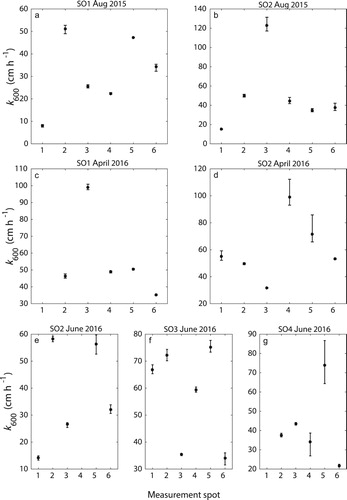
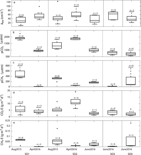
Figure 3. Boxplots of gas transfer velocity (k₆₀₀), pCO₂, pCH₄, and CO₂ and CH₄ emission separated by stream orders (SO) for all sampling occasions; n = number of measurement spots. CO₂ and CH₄ emissions are reported as carbon in g m⁻² d⁻¹. Box shows median value and interquartile range, and whiskers show the adjacent value that is the most extreme data point not considered an outlier. Outliers are illustrated by crosses and are considered above or below 2 standard deviations (2σ) from the mean.

All parameters in our dataset had a nonnormal distribution (Shapiro-Wilks test p < 0.05). To test for correlations between parameters (e.g., U, u′u′, k₆₀₀, Re, pCO₂, pCH4, and CO₂ and CH₄ emissions), we used Pearson’s correlation coefficient tests on log-transformed data. If log-transforming a parameter was not sufficient to approach normal distribution, we performed permutation tests to assess the robustness of Pearson’s correlation coefficients (100 000 iterations). Spectral analysis and data treatments were conducted in MATLAB 2015a and statistical analysis in both MATLAB 2015a and JMP11.

Results

Dissipation rates and variability in k₆₀₀

ADV measurements from all sampling occasions revealed widely variable horizontal flow velocities (Table 1; 0.015–0.83  m s⁻¹). The calculated ε varied from 2.1 × 10⁻⁶ to 1.1 × 10⁻¹ m² s⁻³ (Table 1), with SO3 and SO1 having the highest and lowest log-mean ε, respectively. The corresponding k₆₀₀ varied from 8.1 to 123 cm h⁻¹, with the highest k₆₀₀ observed in SO2. A high within-stream spatial variability in k₆₀₀ was found at every stream reach (Fig. 2, Supplemental Table S2). Within the same stream reach, k₆₀₀ varied by a factor of 2 to 8 between measurement spots (Fig. 2), with the highest variability in SO2 and lowest in SO3 (Fig. 2b and 2f, respectively). The largest within-measurement spot variability was observed during the measurements at SO2 spot 5 during April 2016 (20% from the mean; Supplemental Table S1, Fig. 2). Excluding the extreme cases during high and receding flow, the within-measurement spot variability of k₆₀₀ for all measurements was low, average SD 3% from the mean (n = 35).

Table 1. Mean horizontal current velocity (U), log-mean of dissipation of turbulent kinetic energy (ε), and gas transfer velocity (k₆₀₀) across stream orders (SO) for all sampling occasions, with min−max in parentheses.

SO	No. meas. spots		No. sampling occasions	Total no. measured spots^a	U (m s^−1)	ε (m^2 s^−3)	k600 (cm h^−1)
1	6		2	11	0.29 (0.019−0.84)	8.6×10^−4 (2.1×10^−6–4.6×10^−2)	42.6 (8.1–99)
2	6		3	17	0.23 (0.015–0.82)	2.8×10^−3 (2.0×10^−6–1.1×10^−1)	50.2 (14.2–123)
3	6		1	6	0.23 (0.05–0.61)	4.2×10^−3 (6.5×10^−4–1.5×10^−2)	57.2 (34.0–75.2)
4	6		1	5	0.45 (0.16–0.73)	1.2×10^−3 (1.1×10^−4–1.6×10^−2)	42.2 (21.7–74.0)

^a The total number of successful measurement spots. Three of the total of 42 measurements were discarded because of uncertain data.

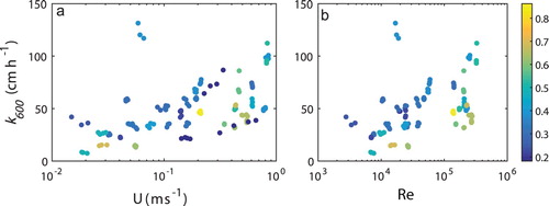
Both u′u′ (a proxy of turbulence; data not shown) and k₆₀₀ were positively correlated with flow speed (Fig. 4a; R = 0.52, p < 0.05, n = 42). Also, k₆₀₀ was correlated with Re (Fig. 4b; R = 0.46, p < 0.05, n = 42). At every flow velocity, however, k₆₀₀ varied by a factor of 2 to 5 (Fig. 4). The channel morphology identified by the hydraulic diameter (Fig 4.) or water depth or widths (data not shown) displayed no clear influence on the relationships between k₆₀₀ and U or Re.

Figure 4. The gas transfer velocity (k₆₀₀) as a function of (a) water current velocity (U) and (b) Reynolds number (Re), both at the logarithmical scale. The color coding reflects the hydraulic diameter (m) of the stream channel for each measurement spot.

CO₂ and CH₄ concentrations and emissions

The highest observed pCO₂ and pCH₄ were found in SO1 (Fig 3b–c, Supplemental Table S2). Considering only summer months during low flow, both pCO₂ and pCH₄ generally decreased with increasing SO. During the highest discharge event (Supplemental Table S1, Apr 2016), pCO₂ and pCH₄ in SO1 were lower than the values observed during occasions with low discharge (Fig. 3b–c, Aug 2015). In SO2, pCH₄ was lower during higher discharge while, by contrast, pCO₂ was higher during high discharge than during low discharge (Supplemental Table S1). SO4 had the highest variability in pCH₄ among the 6 measurement spots.

For the emissions, no consistent pattern was found across SO for either CO₂ or CH₄ (Fig. 3d–e). The highest average emissions were found in SO2 for CO₂ during high discharge and in SO2 for CH₄ during low discharge. The highest within-reach variability in CH₄ emission (as C) was observed in SO4 (8.91–226 mg m⁻² d⁻¹). While pCH₄ tended to decrease with increasing k₆₀₀, no significant correlation was found between pCO₂ and k₆₀₀ (data not shown). The emission of CH₄ showed no correlation with increasing turbulence while CO₂ emission was weakly correlated with turbulence (R = 0.34, p = 0.05, n = 39).

Discussion

Variability in k₆₀₀ and its relation to stream characteristics

Using a consistent methodology across a variety of stream characteristics and stream orders, this study shows a high spatial variability in k₆₀₀, both within stream reaches and across streams of different SOs (Fig. 2 and 3). While both k₆₀₀ and water turbulence (u′u′) were positively related to the mean current velocity, the variability of k₆₀₀ at any given mean current velocity was large (Fig. 4). Also, Re was positively associated with k₆₀₀ (Fig. 4b), illustrating the importance of turbulent flow for gas exchange. Current velocity is related to stream slope, width, depth, and discharge, and these parameters are often included in empirical models for scaling k₆₀₀ in stream systems from local to regional or global scales (Raymond et al. 2012). Our study found no evidence of any clear patterns in k₆₀₀ or turbulence with changing stream width or depth. We observed, however, that at comparable flow speed, a high hydraulic diameter is associated with lower k₆₀₀ rather than a low hydraulic diameter (Fig. 4a), indicating that channel morphology may modulate the relationship between flow speed and k₆₀₀. Although more data are needed before any general conclusions can be drawn, this information suggests that the relationships between stream channel geometry, current velocity, and k₆₀₀ may not be straightforward and may introduce large uncertainties when used for scaling purposes.

The k₆₀₀ values (mean [SD]) measured in this study (k₆₀₀ = 48.1 [26.4] cm h⁻¹) are comparable with values found in the literature of low-order streams. For example, Wallin et al. (2018) estimated a mean k₆₀₀ for all Swedish low-order streams of 39.6 (81.3) cm h⁻¹. Similarly, Butman and Raymond (2011) modeled mean k₆₀₀ for US streams (first- to fourth-order) in the range of 21 to 33 cm h⁻¹. While the mean k₆₀₀ for every stream reach only varied within a factor of 2 in our study (26.7–51.1 cm h⁻¹), the k₆₀₀ across all spot observations displayed high spatial variability, ranging from 7.5 (1.8) m d⁻¹ to 124 (29.8) m d⁻¹; a factor of 16. Furthermore, we observed that k₆₀₀ could vary by as much as a factor of 8 within the same <100  m long stream reach (Fig. 2). For this reason, and because only 6 measurements were conducted at each reach and time point, we consider it unlikely that the mean k₆₀₀ for the different reaches reported here are representative of the respective reach. We attribute the high small-scale spatial variability to the geomorphological heterogeneity, where patches of turbulent riffles and calm pools can be located within a few meters distance. Although a high within-stream spatial variability in k₆₀₀ has been shown in other studies for low-order streams (Crawford et al. 2014, Long et al. 2015), this study is the first documentation at such a small spatial scale and based on direct measurements of water turbulence instead of using floating chambers. The latter point is important and means that k₆₀₀ could be derived at any spot within any stream reach and any stream order, irrespective of its suitability for a chamber deployment. Choosing ADV-based dissipation rate measurements to estimate k₆₀₀ provides an opportunity to investigate small-scale spatiotemporal patterns, patterns that are important for the mechanistic understanding of the control on stream k₆₀₀. Such knowledge is fundamental when k₆₀₀ is scaled based on local measurements to larger landscape units.

Although based on a relatively small dataset, we saw no systematic patterns in either k₆₀₀ or ε across SO (Fig. 3, Table 1), whereas previous studies showed both increasing and decreasing k₆₀₀ with SO (Butman and Raymond 2011, Campeau et al. 2014). Because we were unable to take measurements across all SO in this study from the same sampling occasion, and hence during the same flow regime, the patterns are difficult to assess further; however, our results exemplify that SO (connected to size and widths of the streams) may not be a suitable parameter for estimating k₆₀₀ across landscapes.

A recent study showed that flow intensity is the main controlling factor of k₆₀₀ in streams (Long et al. 2015). Our study supports a positive relationship between flow speed and k₆₀₀, but it further shows that more than half of the variance in k₆₀₀ was not explained by flow speed. In small and shallow low-order stream systems, such as in this study, turbulence is mainly generated by friction forces against the stream bottom and with little influence of anisotropic turbulence (Bluteau et al. 2011). The bottom friction-generated turbulence drives in turn the turbulence at the air–water interface (Gualtieri and Mihailovic 2012). The generation of turbulent motions is therefore probably controlled by bottom roughness, and at increasing discharge and flow speed the turbulent motions and k₆₀₀ are generally enhanced. In addition, channel morphology (e.g., the hydraulic diameter; Fig. 4) may influence the generation of turbulent flow, and thus k₆₀₀. As we observed across all the stream reaches, however, the small-scale spatial variability in k₆₀₀ is high and needs further study. Possibly, accounting for bottom roughness, but also other channel properties (e.g., hydraulic diameter), may help to better understand the linkage between the physical and morphological properties and gas transfer in stream systems.

Estimating k₆₀₀ from ADV-dissipation rate measurements

The main advantage of using direct turbulence measurements to study gas transfer in streams is that k₆₀₀ is measured solely as a physical property and is not inferred from flux measurements from chambers or being dependent on chemical properties of different gases. Although the ADV-based methodology requires many measurements (both laterally and longitudinally distributed), it allows us to study the physical processes specifically to encompass the spatial heterogeneity within a stream reach. By comparison, floating chambers have been used across several slow-flowing systems (Campeau et al. 2014), but recent findings show that using fixed chambers on the water surface introduces additional turbulence and can result in overestimation of gas emissions (Lorke et al. 2015). Tracer injections have mostly been used for lower SOs (Wanninkhof et al. 1990, Wallin et al. 2011, Billett and Harvey 2013) and have the advantage of giving an integrated k₆₀₀ estimate along a certain stream reach. This method, however, requires control on chemical properties of the gases used, proper tracer mixing in the stream channel, discharge rates, and eventual ground water inputs, among other requirements. A clear advantage of the ADV method compared to traditionally used methods is its utility across several SOs, regardless of size and source of turbulence (e.g., wind-driven vs. bottom roughness), enabling methodologically consistent comparisons across the continuum of inland waters.

Deriving values of k₆₀₀ from turbulence measurements is, however, not a standardized method. The within-spot variability in ε was notably low (<3% of the mean) for each measurement occasion, indicating that the precision in the measurements was high. When deriving k₆₀₀ from ε, our approach relies on the application of the eddy-cell model (Lamont and Scott 1970) and the relationship between ε and k₆₀₀ using the proportional constant, C₁ (equation 1(1) ). C₁ has been empirically determined across multiple environmental settings, including artificial systems (Dickey et al. 1984, Asher and Pankow 1986, Moog and Jirka 1999) and natural systems (coastal ocean, lakes and large rivers; Zappa et al. 2007, Vachon et al. 2010, Wang et al. 2015). The observed C₁ found in these studies was 0.1 to 0.5, an expected large range given that the studies represent different measurement setups and environments. C₁ is possibly driven by the measurement depth (Vachon et al. 2010), large scale turbulence (Wang et al. 2015), and the presence of surface film or bubble entrainment (Asher and Pankow 1986). For the present study, we justify our choice of C₁ = 0.43 based on the fact that most studies measuring ε with an ADV near the water surface in natural environments (such as we did) reported C₁ in the range 0.41–0.43 (Zappa et al. 2007, Vachon et al. 2010). In addition, Wang et al. (2015) suggested that under more turbulent conditions (i.e., higher Re), C₁ tends to be higher (<0.5), which should be the case in our streams. Clearly, the proper choice of C₁ (if constant) or its variability among different environmental conditions may have critical implications on the derived k₆₀₀ and calculated gas emissions. Hence, more in-depth investigations on this parameter are needed.

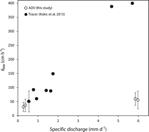
For SO1 and SO2, our estimates of k are based on both ADV dissipation rate measurements (this study) and gas tracer injections from a previous study (Kokic et al. 2015; Fig. 5). The 2 methods were not applied during the same sampling occasions, and, from a fundamental point of view, they cover different spatial scales. The ADV measures water velocity in a 1 cm³ volume, here at 6 spots distributed within a stream reach, whereas the tracer gas injections generates an integrated average k representing the total length of the same stream reach. Hence, a direct comparison between the 2 methods is not justified. Nevertheless, we found that at low discharge, the 2 methods seemed to return similar estimates of k₆₀₀ (Fig. 5). At high discharge, however, the ADV-k method returned much lower k₆₀₀ values than the tracer injection method (SO1: 56 and 399 cm h⁻¹; SO2: 60 and 388 cm h⁻¹ for ADV-k and tracer derived k₆₀₀, respectively). This finding indicates that the relationship between ε and k₆₀₀ seems to hold for low-order streams at low discharge rates, but large discrepancies occurred between the 2 methods at high discharge rates. While horizontal current velocity was high at high discharge, measures of turbulence (ε and u′u′) were for some spot measurements exceptionally low. Possibly, the deeper water in the stream channel during high discharge created a larger distance between the turbulence-creating rough bottom and the water surface at some spots, which may result in less turbulent flow close to the water surface. Another potential cause for this discrepancy at high discharge is the presence of air bubble entrainment, which would increase k₆₀₀ derived from tracer measurements but not from the ADV. To resolve this, further studies are clearly needed that cover a large range in hydrological and morphological conditions and that also investigate the depth profile in dissipation to derive a standardized procedure.

Figure 5. Gas transfer velocity (k₆₀₀) as a function of specific discharge for SO1 and SO2, derived from the eddy cell model (this study; open circles) and tracer injections from Kokic et al. (2015; filled circles). Note that at a k₆₀₀ of ∼50 cm h⁻¹ and a q of ∼0.5 mm d⁻¹, 2 observations overlap, one derived from the tracer-based method and one from the ADV-based method.

Variability in gas concentrations and emissions estimated from ADV-based k₆₀₀

We found the highest gas concentrations in the smallest stream, SO1 (Fig. 3b, Supplemental Table S2), consistent with previous results for CO₂ (Butman and Raymond 2011, Crawford et al. 2013, Wallin et al. 2018). Because first-order streams are closely connected to catchment soils, most water in the stream has recently entered the stream from shallow groundwater, which often is rich in CO₂ (Hope et al. 2004, Öquist et al. 2009, Leith et al. 2015). CO₂ and CH₄ concentrations in SO1–2 were generally higher during low discharge and lower during high discharge. Similarly, a dilution effect likely occurred during the April 2016 sampling occasion because of heavy rains prior to sampling (∼60 mm in the 10 days prior to sampling compared to the annual average of 780 mm [SMHI data]). In SO2 during the discharge event, however, pCO₂ was higher than that of low discharge conditions, most likely the result of CO₂-rich water being flushed out from the lake just upstream (Chmiel et al. 2016). The highest within-reach variability in pCH₄ was observed in SO4. Patches of sediment accumulation with presumably high production of CH₄ at this site may have contributed to the variable water concentrations (Stanley et al. 2016), especially during low flow and low water depth, marked by longer stream water residence times over certain bottom areas and reduced mixing.

We found no clear patterns in gas emission across the different SOs (Fig 3d–e). SO2 had the highest CO₂ emission during the discharge event, which can be connected to the high pCO₂ values from the upstream lake. The emission of CH₄ in SO4 was high and highly variable, most likely attributable to the pCH₄ because the pCH₄ was much higher at this site compared to the other sites, whereas k₆₀₀ was lower. The highest CH₄ emission was found in SO2 during low discharge, where the combination of both high concentration and k₆₀₀ contributes to these emission rates. The coefficient of variation for pCO₂, pCH₄, and k₆₀₀ within each stream reach (i.e., across the 6 measured spots) showed that the variability in k₆₀₀ always exceeded the variability in pCO₂ and pCH₄, with the exception of pCH₄ in SO4 (Supplemental Table S2). This finding may suggest that CO₂ and CH₄ emissions are primarily driven by the physical rate of gas exchange and, to a lesser extent, by the degree of oversaturation of CO₂ or CH₄. As indicated by the exception of pCH₄ in SO4 (Supplemental Table S2), however, CH₄ emissions in individual stream sections could be more limited by the production and supply of CH₄ rather than k. Different controls (biological vs. physical) on CO₂ and CH₄ emission rates have been found in other stream studies (Gómez-Gener et al. 2015, Natchimuthu et al. 2017).

Conclusions

Here we show high spatial variability in k derived by direct turbulence measurements along and across low-order streams. Understanding this variability is an important step to reducing the uncertainty in existing gas transfer models for stream systems. Although further method development is needed, using direct turbulence measurements by an ADV is a promising method to explore the small-scale variability in k. This information is needed to construct physically founded models of k₆₀₀ suitable across all types of stream/river sizes and channel morphologies. Given the potential of the methodology, more studies are needed to evaluate and standardize the approach. We further conclude that high discharge rates deserve particular attention in future studies, potentially by conducting simultaneous measurements with an independent approach. Based on the low within-spot variability measured in this study (Fig. 2), we recommend that future studies conduct ADV measurements over shorter time periods at each measurement spot (e.g., 10–15  min instead of 40  min). Shorter times will allow measurements at more spots across the reach of interest and thereby derive more reliable mean-reach k₆₀₀ and more information about controls of the spatial variability in k₆₀₀. Similar to previous studies, our results show increases in k₆₀₀ and gas emissions with increasing flow; however, the relationship was rather weak and not related to commonly used channel geometry measures as stream width or depth, and only weakly related to hydraulic diameter. Future studies should investigate the influence of bottom roughness and channel morphology on k₆₀₀.

Acknowledgements

We thank Ron Coleman and Emma Åkerman Fulford for extensive help with the field-sampling campaigns. Financial support is acknowledged by SS and ES from the Swedish Research Council, and by SS from Formas. The research leading to these results has received funding from the European Research Council under the European Union's Seventh Framework Programme (FP7/2007-2013)/ERC grant agreement n° 336642. The study also benefitted from funding from Knut and Alice Wallenberg foundation. Data used in this study are available at http://urn.kb.se/resolve?urn = urn:nbn:se:uu:diva-338568.

ORCID

Jovana Kokic http://orcid.org/0000-0002-8763-3139

Erik Sahlée http://orcid.org/0000-0002-6183-9876

Dominic Vachon http://orcid.org/0000-0003-1157-5240

Marcus B. Wallin http://orcid.org/0000-0002-3082-8728

References

- Alin S, Rasera M, Salimon C, Richey J, Holtgrieve G, Krusche A, Snidvongs A. 2011. Physical controls on carbon dioxide transfer velocity and flux in low-gradient river systems and implications for regional carbon budgets. J Geophys Res-Biogeo. 116:G01009. doi: 10.1029/2010JG001398
- Asher WE, Pankow JF. 1986. The interaction of mechanically generated turbulence and interfacial films with a liquid phase controlled gas/liquid transport process. Tellus B. 38B:305–318.
- Billett MF, Harvey FH. 2013. Measurements of CO2 and CH4 evasion from UK peatland headwater streams. Biogeochemistry. 114:165–181. doi: 10.1007/s10533-012-9798-9
- Bluteau CE, Jones NL, Ivey GN. 2011. Estimating turbulent kinetic energy dissipation using the inertial subrange method in environmental flows. Limnol Oceanogr-Meth. 9:302–321. doi: 10.4319/lom.2011.9.302
- Butman D, Raymond P. 2011. Significant efflux of carbon dioxide from streams and rivers in the United States. Nat Geosci. 4:839–842. doi: 10.1038/ngeo1294
- Campeau A, Lapierre J-F, Vachon D, del Giorgio PA. 2014. Regional contribution of CO2 and CH4 fluxes from the fluvial network in a lowland boreal landscape of Québec. Glob Biogeochem Cy. 28:57–69. doi: 10.1002/2013GB004685
- Chmiel HE, Kokic J, Denfeld BA, Einarsdóttir K, Wallin MB, Koehler B, Isidorova A, Bastviken D, Ferland M-È, Sobek S. 2016. The role of sediments in the carbon budget of a small boreal lake. Limnol Oceanogr. 61:1814–1825. doi: 10.1002/lno.10336
- Clark JF, Wanninkhof R, Schlosser P, Simpson HJ. 1994. Gas exchange rates in the tidal Hudson river using a dual tracer technique. Tellus B. 46:274–285. doi: 10.3402/tellusb.v46i4.15802
- Cook PG, Lamontagne S, Berhane D, Clark JF. 2006. Quantifying groundwater discharge to Cockburn River, southeastern Australia, using dissolved gas tracers 222Rn and SF6. Water Resour Res. 42:W10411.
- Crawford JT, Lottig NR, Stanley EH, Walker JF, Hanson PC, Finlay JC, Striegl RG. 2014. CO2 and CH4 emissions from streams in a lake-rich landscape: patterns, controls and regional significance. Glob Biogeochem Cy. 28:197–210. doi: 10.1002/2013GB004661
- Crawford JT, Striegl RG, Wickland KP, Dornblaser MM, Stanley EH. 2013. Emissions of carbon dioxide and methane from a headwater stream network of interior Alaska. J Geophys Res-Biogeo. 118:482–494. doi: 10.1002/jgrg.20034
- Day T. 1976. Precision of salt dilution gauging. J Hydrol. 31:293–306. doi: 10.1016/0022-1694(76)90130-X
- Denfeld BA, Wallin MB, Sahlee E, Sobek S, Kokic J, Chmiel HE, Weyhenmeyer GA. 2015. Temporal and spatial carbon dioxide concentration patterns in a small boreal lake in relation to ice-cover dynamics. Boreal Environ Res. 20:679–692.
- Dickey TD, Hartman B, Hammond D, Hurst E. 1984. A laboratory technique for investigating the relationship between gas transfer and fluid turbulence. In: Brutsaert W, Jirka GH, editors. Gas transfer at water surfaces. Dordrecht: Springer Netherlands; p. 93–100.
- Dinsmore KJ, Billett MF, Skiba UM, Rees RM, Drewer J, Helfter C. 2010. Role of the aquatic pathway in the carbon and greenhouse gas budgets of a peatland catchment. Glob Change Biol. 16:2750–2762. doi: 10.1111/j.1365-2486.2009.02119.x
- Einarsdottir K, Wallin MB, Sobek S. 2017. High terrestrial carbon load via groundwater to a boreal lake dominated by surface water inflow. J Geophys Res-Biogeo. 122:15–29. doi: 10.1002/2016JG003495
- Gålfalk M, Bastviken D, Fredriksson S, Arneborg L. 2013. Determination of the piston velocity for water-air interfaces using flux chambers, acoustic Doppler velocimetry, and IR imaging of the water surface. J Geophys Res-Biogeo. 118:770–782. doi: 10.1002/jgrg.20064
- Genereux DP, Hemond HF. 1990. Naturally occuring radon 222 as a tracer for streamflow generation: steady state methodology and field example. Water Resour Res. 26:3065–3075.
- Gómez-Gener L, Obrador B, von Schiller D, Marcé R, Casas-Ruiz JP, Proia L, Acuña V, Catalán N, Muñoz I, Koschorreck M. 2015. Hot spots for carbon emissions from Mediterranean fluvial networks during summer drought. Biogeochemistry. 125:409–426. doi: 10.1007/s10533-015-0139-7
- Goring DG, Nikora VI. 2002. Despiking acoustic doppler velocimeter data. J Hydraul Eng. 128:117–126. doi: 10.1061/(ASCE)0733-9429(2002)128:1(117)
- Gualtieri C, Mihailovic DT. 2012. Fluid mechanics of environmental interfaces. Boca Raton (FL): CRC Press.
- Högström U. 1996. Review of some basic characteristics of the atmospheric surface layer. Bound-Lay Meteorol. 78:215–246. doi: 10.1007/BF00120937
- Hope D, Palmer S, Billett M, Dawson J. 2001. Carbon dioxide and methane evasion from a temperate peatland stream. Limnol Oceanogr. 46:847–857. doi: 10.4319/lo.2001.46.4.0847
- Hope D, Palmer S, Billett M, Dawson J. 2004. Variations in dissolved CO2 and CH4 in a first-order stream and catchment: an investigation of soil-stream linkages. Hydrol Proc. 18:3255–3275. doi: 10.1002/hyp.5657
- Jähne B, Haußecker H. 1998. Air-water gas exchange. Annu Rev Fluid Mech. 30:443–468. doi: 10.1146/annurev.fluid.30.1.443
- Jähne B, Heinz G, Dietrich W. 1987. Measurement of diffusion-coefficients of sparigly soluble gases in water. J Geophys Res-Oceans. 92:10767–10776. doi: 10.1029/JC092iC10p10767
- Kokic J, Wallin MB, Chmiel HE, Denfeld BA, Sobek S. 2015. Carbon dioxide evasion from headwater systems strongly contributes to the total export of carbon from a small boreal lake catchment. J Geophys Res-Biogeo. 120:13–28. doi: 10.1002/2014JG002706
- Lamont JC, Scott DS. 1970. An eddy cell model of mass transfer into the surface of a turbulent liquid. AIChE J. 16:513–519. doi: 10.1002/aic.690160403
- Lee X, Massman W, Law B. 2004. Handbook of micrometeorology - a guide for surface flux measurement and analysis. USA: Kluwer Academic.
- Leith FI, Dinsmore KJ, Wallin MB, Billett MF, Heal KV, Laudon H, Öquist MG, Bishop K. 2015. Carbon dioxide transport across the hillslope–riparian–stream continuum in a boreal headwater catchment. Biogeosciences. 12:1881–1892. doi: 10.5194/bg-12-1881-2015
- Lide DR, Frederikse HPR. 1995. Handbook of chemistry and physics. 76th ed. Boca Raton (FL): CRC Press.
- Long H, Vihermaa L, Waldron S, Hoey T, Quemin S, Newton J. 2015. Hydraulics are a first order control on CO2 efflux from fluvial systems. J Geophys Res-Biogeo. 120:1912–1922. doi: 10.1002/2015JG002955
- Lorke A, Bodmer P, Noss C, Alshboul Z, Koschorreck M, Somlai-Haase C, Bastviken D, Flury S, McGinnis DF, Maeck A, et al. 2015. Technical note: drifting versus anchored flux chambers for measuring greenhouse gas emissions from running waters. Biogeosciences. 12:7013–7024. doi: 10.5194/bg-12-7013-2015
- Lorke A, Peeters F. 2006. Toward a unified scaling relation for interfacial fluxes. J Phys Oceanogr. 36:955–961. doi: 10.1175/JPO2903.1
- Moog DB, Jirka GH. 1999. Air–water gas transfer in uniform channel flow. J Hydraul Eng. 125:3–10. doi: 10.1061/(ASCE)0733-9429(1999)125:1(3)
- Natchimuthu S, Wallin MB, Klemedtsson L, Bastviken D. 2017. Spatio-temporal patterns of stream methane and carbon dioxide emissions in a hemiboreal catchment in southwest Sweden. Sci Rep. 7:39729.
- Öquist M, Wallin M, Seibert J, Bishop K, Laudon H. 2009. Dissolved inorganic carbon export across the soil/stream interface and its fate in a boreal headwater stream. Environ Sci Technol. 43:7364–7369. doi: 10.1021/es900416h
- Raymond P, Cole JJ. 2001. Technical notes and comments: gas exchange in rivers and estuaries: choosing a gas transfer velocity. Estuaries. 24:312–317. doi: 10.2307/1352954
- Raymond P, Hartmann J, Lauerwald R, Sobek S, McDonald C, Hoover M, Butman D, Striegl RG, Mayorga E, Humborg C, et al. 2013. Global carbon dioxide emissions from inland waters. Nature. 503:355–359. doi: 10.1038/nature12760
- Raymond P, Zappa CJ, Butman D, Bott TL, Potter J, Mulholland P, Laursen AE, McDowell WH, Newbold D. 2012. Scaling the gas transfer velocity and hydraulic geometry in streams and small rivers. Limnol Oceanogr-Fluid Environ. 2:41–53. doi: 10.1215/21573689-1597669
- Stanley EH, Casson NJ, Christel ST, Crawford JT, Loken LC, Oliver SK. 2016. The ecology of methane in streams and rivers: patterns, controls, and global significance. Ecol Monogr. 86:146–171. doi: 10.1890/15-1027
- Striegl RG, Dornblaser MM, Mcdonald CP, Rover JR, Stets EG. 2012. Carbon dioxide and methane emissions from the Yukon River system. Glob Biogeochem Cy. 26:GB0E05. doi: 10.1029/2012GB004306
- Tokoro T, Kayanne H, Watanabe A, Nadaoka K, Tamura H, Nozaki K, Kato K, Negishi A. 2008. High gas-transfer velocity in coastal regions with high energy-dissipation rates. J Geophys Res-Oceans. 113:C11006. doi: 10.1029/2007JC004528
- Vachon D, Prairie YT, Cole JJ. 2010. The relationship between near-surface turbulence and gas transfer velocity in freshwater systems and its implications for floating chamber measurements of gas exchange. Limnol Oceanogr. 55:1723–1732. doi: 10.4319/lo.2010.55.4.1723
- Wallin MB, Campeau A, Audet J, Bastviken D, Bishop K, Kokic J, Laudon H, Lundin E, Löfgren S, Natchimuthu S, et al. 2018. Carbon dioxide and methane emissions of Swedish low-order streams – a national estimate and lessons learnt from more than a decade of observations. Limnol Oceanogr-Lett. 3:156–167. doi: 10.1002/lol2.10061
- Wallin MB, Oquist MG, Buffam I, Billett MF, Nisell J, Bishop KH. 2011. Spatiotemporal variability of the gas transfer coefficient KCO2 in boreal streams: implications for large scale estimates of CO2 evasion. Glob Biogeochem Cy. 25:GB3025. doi: 10.1029/2010GB003975
- Wang B, Liao Q, Fillingham JH, Bootsma HA. 2015. On the coefficients of small eddy and surface divergence models for the air-water gas transfer velocity. J Geophys Res-Oceans. 120:2129–2146. doi: 10.1002/2014JC010253
- Wanninkhof R. 1992. Relationship between wind speed and gas exchange over the ocean. J Geophys Res-Oceans. 97:7373–7382. doi: 10.1029/92JC00188
- Wanninkhof R. 2014. Relationship between wind speed and gas exchange over the ocean revisited. Limnol Oceanogr-Meth. 12:351–362. doi: 10.4319/lom.2014.12.351
- Wanninkhof R, Mulholland PJ, Elwood JW. 1990. Gas exchange rates for a first-order stream determined with deliberate and natural tracers. Water Resour Res. 26:1621–1630.
- Weiss RF. 1974. Carbon dioxide in water and seawater: the solubility of a non-ideal gas. Mar Chem. 2:203–215. doi: 10.1016/0304-4203(74)90015-2
- Zappa CJ, McGillis WR, Raymond PA, Edson JB, Hintsa EJ, Zemmelink HJ, Dacey JWH, Ho DT. 2007. Environmental turbulent mixing controls on air–water gas exchange in marine and aquatic systems. Geophys Res Lett. 34:L10601.