The drawdown phase of dam decommissioning is a hot moment of gaseous carbon emissions from a temperate reservoir

ABSTRACT

Dam decommissioning (DD) is a viable management option for thousands of ageing dams. Reservoirs are large carbon sinks, and reservoir drawdown results in important carbon dioxide (CO₂) and methane (CH₄) emissions. We studied the effects of DD on CO₂ and CH₄ fluxes from impounded water, exposed sediment, and lotic water before, during, and 3–10 months after drawdown of the Enobieta Reservoir, north Iberian Peninsula. During the study period, impounded water covered 0–100%, exposed sediment 0–96%, and lotic water 0–4% of the total reservoir area (0.14 km²). Areal CO₂ fluxes in exposed sediment (mean [SE]: 295.65 [74.90] mmol m⁻² d⁻¹) and lotic water (188.11 [86.09] mmol m⁻² d⁻¹) decreased over time but remained higher than in impounded water (−36.65 [83.40] mmol m⁻² d⁻¹). Areal CH₄ fluxes did not change over time and were noteworthy only in impounded water (1.82 [1.11] mmol m⁻² d⁻¹). Total ecosystem carbon (CO₂ + CH₄) fluxes (kg CO₂-eq d⁻¹) were higher during and after than before reservoir drawdown because of higher CO₂ fluxes from exposed sediment. The reservoir was a net sink of carbon before reservoir drawdown and became an important emitter of carbon during the first 10 months after reservoir drawdown. Future studies should examine mid- and long-term effects of DD on carbon fluxes, identify the drivers of areal CO₂ fluxes from exposed sediment, and incorporate DD in the carbon footprint of reservoirs.

KEYWORDS:

• ageing dams
• carbon dioxide fluxes
• dam removal
• exposed sediment
• reservoir drawdown
• water reservoirs

Introduction

Reservoirs influence the global carbon (C) cycle and climate system because they are large sinks of organic C and great emitters of carbon dioxide (CO₂) and methane (CH₄) greenhouse gases (GHGs; Downing et al. 2008, Deemer et al. 2016, Mendonça et al. 2017). Emissions of GHGs during the operational phase of reservoirs, ∼0.8 Pg CO₂ equivalents (CO₂-eq) yr⁻¹ (Deemer et al. 2016), have been included in the global inventories of anthropogenic GHGs (IPCC 2019) because they play a significant role in global warming. The global C emissions from reservoirs are lower than the organic C burial in their sediments (Deemer et al. 2016, Mendonça et al. 2017), although this finding has been recently challenged (Keller et al. 2021). In addition, during the removal of a dam and its ancillary facilities, (i.e., dam decommissioning), the large stocks of organic C in the sediments of the reservoir may decompose and emit more CO₂ and CH₄ (Pacca 2007, Perera et al. 2021).

Dam decommissioning (DD) is becoming a credible management solution for tens of thousands of dams that have reached or exceeded their engineered life expectancies of 50–100 years (Doyle et al. 2003, Stanley and Doyle 2003, Perera et al. 2021). Dams are removed for several reasons, including environmental restoration, increasing maintenance costs, gradual reservoir sedimentation, and public safety (Perera et al. 2021). The process of DD has gained high research interest, which has focused mostly on the effects of river connectivity on ecological processes such as migration and dispersal of living organisms (Bednarek 2001, Marks et al. 2010, Bellmore et al. 2019). Although reservoir sediments are important repositories of organic C, previous studies have not examined the fate of that sediment organic C following DD (Pacca 2007). Dam decommissioning may be a relevant component of the C balance in a reservoir because reservoir drawdown is hot moment for the decomposition of sediment organic C to CO₂ and CH₄ (Deshmukh et al. 2018, Keller et al. 2021, Paranaíba et al. 2021).

The reservoir drawdown phase of DD is likely to first increase CO₂ and CH₄ fluxes from a reservoir through the formation of shallow waters (Harrison et al. 2017, Deshmukh et al. 2018, Li et al. 2020). Small patches of shallow waters can emit, for instance, 75% and 90% of, respectively, the annual CO₂ and CH₄ fluxes from reservoirs (Harrison et al. 2017, Deshmukh et al. 2018). Approximately 35% of total CH₄ fluxes from the surface waters of reservoirs is emitted via diffusion while 65% is emitted via ebullition (Deemer et al. 2016), which is higher in shallow waters (Baulch et al. 2011). Shallow waters emit higher areal C fluxes due to conditions such as increased aeration and temperature that facilitate gas production in sediments, and shallow depth that results in low hydrostatic pressure and readily allows gases to be transported to the overlying water layer and the water—atmosphere interface (Harrison et al. 2017, Li et al. 2020). Dam decommissioning may promote C emissions to the atmosphere because of the increased areal extension in shallow waters resulting from reservoir drawdown.

Reservoir drawdown can furthermore produce high C fluxes when it exposes sediments to the atmosphere. Exposed sediment is a hotspot for CO₂ emissions, whose areal fluxes in reservoirs (4–1533 mmol m⁻² d⁻¹; Gómez-Gener et al. 2016, Jin et al. 2016, Obrador et al. 2018) are higher than CO₂ fluxes from surface waters of lentic waters (18–55 mmol m⁻² d⁻¹; Raymond et al. 2013, Deemer et al. 2016, Holgerson and Raymond 2016), and even comparable to areal CO₂ fluxes from lotic water (120–633 mmol m⁻² d⁻¹; Raymond et al. 2013, Borges et al. 2015, Gómez-Gener et al. 2015). Lotic waters emit higher C fluxes than impounded water because of their highly turbulent water columns and, hence, higher gas exchange coefficients (Gómez-Gener et al. 2015). Furthermore, the higher CO₂ emissions from exposed sediment are related to a closer coupling of CO₂ production and fluxes and increased CO₂ production due to high oxygen availability (Fromin et al. 2010, Keller et al. 2020).

Increased redox potentials in exposed sediment reduce CH₄ production and increase CH₄ oxidation, which results in lower CH₄ fluxes. Thus, CH₄ fluxes from exposed sediment (0.1–1 mmol m⁻² d⁻¹; Yang et al. 2014, Gómez-Gener et al. 2015, Deshmukh et al. 2018) are lower than CH₄ fluxes from lotic waters (4.2 [8.4] mmol m⁻² d⁻¹; Stanley et al. 2016) and surface waters of lakes and reservoirs (3–10 mmol m⁻² d⁻¹; Deemer et al. 2016). Fluxes of CH₄ from a flooded site may even be 3 orders of magnitude higher than CH₄ fluxes from a nonflooded site of the same reservoir (Yang et al. 2014). Although areal CO₂ fluxes are higher than CH₄ fluxes from reservoirs, CH₄ has a global warming potential 25 times higher than that of CO₂ over a span of 100 years (IPCC 2013); thus, 79% of the annual CO₂-eq emissions from reservoirs occurs as CH₄ (Deemer et al. 2016). In summary, when exposed sediment replaces impounded water during DD, CO₂ emissions may increase, whereas CH₄ emissions may decrease. However, to our knowledge, no empirical evidence exists on the effects of DD on C fluxes in reservoirs. This knowledge would help inform regional and global scale estimates of the C footprint of reservoirs and their perception as a C-neutral source of energy (Barros et al. 2011).

Here, we assessed short-term effects of DD on CO₂ and CH₄ fluxes before, during, and after drawdown of a temperate reservoir. We measured CO₂ and CH₄ fluxes in exposed sediment, deep and shallow zones of impounded water, and lotic water. We hypothesized a temporal change in CO₂ and CH₄ fluxes for the 3 environments along reservoir drawdown, CO₂ fluxes highest in exposed sediment, CH₄ fluxes highest in impounded water, higher CO₂ and CH₄ fluxes from the shallow zone than the deep zone of impounded water, and higher ecosystem C fluxes due to higher areal C fluxes from exposed sediment and lotic water after reservoir drawdown.

Materials and methods

Study site

The Enobieta Reservoir is in the valley of Artikutza (Navarre, northern Iberian Peninsula), where human activities have been restricted since 1919, when the municipality of Donostia-San Sebastián bought the land to ensure the supply of high-quality drinking water. The mean annual air temperature is 12.2 °C with an average rainfall of 2064 mm yr⁻¹ (average 1954–2019; Gobierno de Navarra 2019). The dam was constructed between 1947 and 1953 on the Enobieta Stream. The reservoir had an initial storage capacity of 2.66 hm³, length of 1.1 km, maximum depth of 25.5 m, a concrete dam height of 42 m, and an area of 0.14 km². Geotechnical problems appeared during its construction, forcing a reduction in its storage capacity to 1.40 hm³, and the construction of a larger reservoir (Añarbe Reservoir, 43.8 hm³) downstream in 1976, after which Enobieta Reservoir was no longer used as a water supply facility (Larrañaga et al. 2019). In addition, Artikutza is part of the Natura 2000 Network and, since 2014, is a special conservation zone. The high conservation status of the valley and the structural instability of the dam led to a DD plan of the Enobieta Reservoir, a process that began in 2017 and extended through and 2019 (Supplemental Fig. S1). To date, the decommissioning has been partial; the reservoir has been completely emptied of water and the river runs freely through a hole in the dam, but the concrete structure of the dam (the physical structure retaining the water) is still standing.

Sampling design

We measured CO₂ and CH₄ fluxes in 3 environments—impounded water, exposed sediment, and lotic water—before, during, and after reservoir drawdown. We conducted 8 sampling campaigns on 16 June 2016, 7 July 2018, 10 September 2018, 22 October 2018, 21 January 2019, 9 April 2019, 2 July 2019, and 18 February 2020 (Table 1, Supplemental Fig. S1). Exposed sediment and lotic water completely replaced impounded water on 25 February 2019. The campaigns conducted before 25 February 2019 correspond to the periods Before and During reservoir drawdown, while the campaigns after this date correspond to the period After reservoir drawdown. Thus, we sampled 2 times prior to drawdown (day −984 and −233), 3 times during drawdown (days −168, −126, and −35), and 3 times after drawdown was complete (day 43, 127, and 358). We identified these days by taking the sampling date minus 25 February 2019 (for instance, 16 June 2016–25 February 2019 = −984 days; Table 1).

Table 1. Sampling campaigns, sampling date (day/month/year), time (d) before or after exposed sediment completely replaced impounded water, phase of DD (pre = before, peri = during, post = after), average reservoir water depth (RWD), surface area and percentage (%) area of each environment, and zone (DS = deep and shallow, S = only shallow) sampled within impounded water, transects (A, B, C, and D) sampled for exposed sediment, (n is the sample size of CO₂ fluxes in exposed sediment while the sample size for CH₄ fluxes is 3 times less than that of CO₂ for each sampling), NA = not applicable.

Sampling date	Time	Phase	RWD (m)	Impounded water			Exposed sediment			Running water
				Area (m^2)	% area	Depth	Area (m^2)	% area	Transect (n)	Area (m^2)	% area
16/06/16	−984	pre	20	141 400	100	DS	0	0	NA	0	0
07/07/18	−233	pre	19.8	140 800	99.6	DS	526	0.4	A (3)	74	0.1
10/09/18	−168	peri	14.8	101 200	71.5	DS	39 385	28	ABC (27)	815	0.5
22/10/18	−126	peri	9.8	71 500	50.6	DS	69 400	48.4	ABC (27)	1500	1
21/01/19	−35	peri	4.8	15 000	10.6	S	122 500	86.6	ABC (27)	3900	2.8
09/04/19	43	post	0	0	0	NA	135 800	96	ABCD (45)	5600	4
02/07/19	127	post	0	0	0	NA	135 800	96	ABCD (45)	5600	4
18/02/20	358	post	0	0	0	NA	135 800	96	ABCD (45)	5600	4

Impounded water was sampled from day −984 to day −35 (i.e., when it was present) in 2 zones: deep water (>4 m) and shallow water (<4 m; Harrison et al. 2017; Fig. 1, Table 1, Supplemental Fig. S1). The location of the shallow water zone changed over time as the water level decreased along drawdown. Before exposed sediment and lotic water completely replaced impounded water (day −233 to −35), we measured CO₂ and CH₄ fluxes in lotic water at the stream–reservoir transition inlet (1 site). After complete reservoir drawdown (day 43–358), we measured the fluxes in lotic water at 2 sites across the reservoir. For both impounded water and lotic water, we measured CO₂ and CH₄ fluxes in triplicate (3 samples at each site).

Figure 1. Simplified schematic and photographic view of the sampling design showing the state of Enobieta Reservoir when (a) it was full: photo taken on day −233, July 2018; and (b) when it was empty: photo taken on day 358, February 2020. The scheme shows the 3 sampled environments: exposed sediment, impounded water, and running water. The red dashed lines are the cross-sectional transects used to measure CO₂ and CH₄ fluxes from exposed sediment. The numbers in brackets are the number of sites sampled for each transect of exposed sediment on each day. Photos taken by M. Amani and B. Obrador.

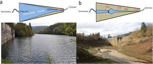
We sampled CO₂ and CH₄ fluxes in exposed sediment from day −233 to day 358 (when it was present; Table 1). To measure CO₂ and CH₄ fluxes in exposed sediment, we used 4 cross-sectional transects (A, B, C, and D; Fig. 1) comprising between 1 and 5 sites (Supplemental Table S1). We measured 3 CO₂ fluxes and 1 CH₄ flux at each site. The number of transects and the number of sites for some transects increased with time as water retracted from the edge to the center and toward the dam of the reservoir. For instance, because impounded water covered most of the reservoir on day −233, we had only transect A with 1 site (thus, the sample size [n] in this campaign was 3 for CO₂ and 1 for CH₄). Moreover, the number of sites among transects varied because the distance from the center to the edge of the reservoir differed across the reservoir. Consequently, the number and length of transects changed with reservoir drawdown (Table 1). During reservoir drawdown (day −168 to −35), we used 3 transects (A, B, and C) with 3 sites each (n = 27 for CO₂ and n = 9 for CH₄). After reservoir drawdown (from day 43 onward), we used 4 transects, with 3 (A and D), 4 (B), and 5 (C) sites each (n = 45 for CO₂ and n = 15 for CH_4; Fig. 1, Supplemental Table S1).

Determination of CO₂ fluxes

We determined CO₂ fluxes from exposed sediment and impounded water using the chamber method (Frankignoulle 1988). We measured CO₂ fluxes from exposed sediment with an enclosed opaque soil respiration chamber (SRC-1, PP-Systems, Amesbury, MA, USA). For impounded water, we estimated CO₂ fluxes across the water–air interface with a custom-made floating enclosed opaque chamber. We monitored the partial pressure of CO₂ (pCO₂) in the chambers every second with an infrared gas analyser (IRGA-EGM-5, PP-Systems, 1% accuracy). We waited for pCO₂ in chambers to change by at least 10 µatm, which took 120–300 s in exposed sediment and 300–600 s in impounded water. We calculated CO₂ fluxes from exposed sediment and impounded water by a linear regression of pCO₂ in the chambers over time corrected for temperature and pressure as: (1) $F{\mathrm{C}\mathrm{O}}_2=\left({\displaystyle \frac{dp{\mathrm{C}\mathrm{O}}_2}{dt}}\right)\left({\displaystyle \frac{V}{RTS}}\right),$(1) where FCO₂ is CO₂ flux (mol m⁻² d⁻¹), dpCO₂/dt is the slope of the regression of pCO₂ in the chamber over time (atm d⁻¹), V is the volume of the chamber (1.171 × 10⁻³ m³ for exposed sediment, 0.027 m³ for impounded water), S is the area of the chamber (7.8 × 10⁻³ m² for exposed sediment and 0.194 m² for impounded water), T is temperature (K), and R is the ideal gas constant (m³ atm K⁻¹ mol⁻¹). All fluxes reported here follow the convention that efflux to the atmosphere corresponds to a positive flux, and uptake or influx corresponds to a negative flux.

We determined the direction and magnitude of CO₂ fluxes from lotic water by applying Fick’s first law of gas diffusion: (2) $F{\mathrm{C}\mathrm{O}}_{2stream}=k{\mathrm{C}\mathrm{O}}_2\times \text{β}\times \left(p{\mathrm{C}\mathrm{O}}_{2w}-p{\mathrm{C}\mathrm{O}}_{2a}\right),$(2) where FCO_2stream is the CO₂ flux from lotic water (mol m⁻² d⁻¹), kCO₂ is the transfer velocity of CO₂ (m d⁻¹), β is the solubility coefficient of CO₂ (mol m⁻³ atm⁻¹), and pCO_2w and pCO_2a are, respectively, the partial pressures of CO₂ (atm) in surface water and air.

We determined pCO_2w and pCO_2a in triplicate at each sampling site. The pCO_2w was determined by means of a membrane gas exchanger (MiniModule, Liqui-Cel, 3M, Maplewood, MN, USA) coupled to an IRGA. We circulated sampled water via gravity through the membrane contactor at a rate of 300 mL min⁻¹ while recirculating an enclosed volume of gas between the membrane and the IRGA. We determined the solubility of CO₂, for the temperature and salinity of each sample (Bastviken et al. 2004). We estimated kCO₂ (m d⁻¹) in the lotic water as: (3) $k{\mathrm{C}\mathrm{O}}_2=k_{600}{\left({\displaystyle \frac{Sc{\mathrm{C}\mathrm{O}}_2}{600}}\right)}^{-\frac{2}{3}},$(3) where ScCO₂ is the Schmidt number of CO₂ (dimensionless) and k₆₀₀ (m d⁻¹) is k of CO₂ at a Schmidt number (Sc) of 600, (4) $k_{600}=5.14\times d\times {\displaystyle \frac{Vel}{d^{1.33}}{\left({\displaystyle \frac{600}{Sc{\mathrm{C}\mathrm{O}}_2}}\right)}^{-\frac{2}{3}},}$(4) d is depth of the water column (m) and Vel denotes the water velocity (m s⁻¹), noting that this equation is an empirical adjustment for k₆₀₀ in lotic water.

We estimated the velocity of lotic water by the time–conductivity curve that we obtained in instantaneous additions of a tracer (NaCl) at a turbulent point in the channel, 200 m downstream of the point of addition, using a field conductivity meter (WTW 340i, Germany). We recorded changes in electrical conductivity generated by the tracer pulse then used the changes to calculate the speed by dividing the distance by time that electrical conductivity takes to reach the maximum peak (Gordon et al. 2004).

Determination of CH₄ fluxes

Determination of diffusive CH₄ fluxes in water

We determined diffusive CH₄ fluxes from impounded water and lotic water using the gradient of pCH₄ between water and air. We collected 3 samples of pCH₄ in surface water at each sampling site using the headspace technique equilibrated in situ with air (Bastviken et al. 2004). Briefly, we collected 30 mL of water with a 60 mL plastic syringe, which created a headspace with ambient air at 1:1 ratio (collected water:ambient air). We manually shook the syringe for 1 min and then submerged it at each sampling site for 5 min to maintain constant equilibration temperature. Thereafter, we transferred 20 mL of the gas mixture from the plastic syringe to a pre-evacuated vial (Exetainer, Labco Ltd., Lampeter, UK). We took ambient air samples to correct for CH₄ concentration in the headspace.

In the laboratory, we determined pCH₄ in the gaseous mixture using a gas chromatograph equipped with a Flame Ionising Detector (FID; 7820A GC, Agilent, Santa Clara, CA, USA), with an accuracy of 4%. We routinely ran 6 point standard curves obtained from a standard of 15 ppm CH₄ (Crystal, Air Liquide SA, Paris, France).

We determined diffusive CH₄ fluxes as for CO₂ (equation 2). In impounded water, the CH₄ transfer coefficient (kCH₄, in m d⁻¹) was obtained as: (5) $k{\mathrm{C}\mathrm{H}}_4=k_{600}{\left({\displaystyle \frac{Sc{\mathrm{C}\mathrm{H}}_4}{600}}\right)}^{-0.5},$(5) with (6) $k_{600}=0.228\times U_{10}^{2.2}+0.168,$(6) where ScCH₄ is the Schmidt number for CH₄ and U₁₀ corresponds to the wind speed (m s⁻¹) at a height of 10 m above impounded water. To find U₁₀ we measured the wind speed in situ at 1 m with a portable anemometer (Kestrel 4000, Boothwyn, PA, USA) and converted it to U₁₀ following Crusius and Wanninkhof (2003). We determined ScCH₄ in impounded water and lotic water at the measured water temperature (Howard and Howard 1993, Gómez-Gener et al. 2015). We calculated CH₄ fluxes from lotic water the same way we calculated CO₂ fluxes, using ScCH₄ instead of ScCO₂ in equation 3 to estimate kCH₄.

Determination of ebullitive CH₄ fluxes from impounded water

We measured ebullitive CH₄ fluxes from impounded water with 8 inverted funnel collectors: 4 in deep water and 4 in shallow water. We maintained the funnels for 6–23 h (DelSontro et al. 2010) to get a measurable flux (i.e., a detectable signal). The funnels (collection area of 0.44 m²) had a collector bottle where the gas accumulated during the entire sampling period. We closed the collectors of each funnel underwater and weighed them on the shore to determine the volume of gas, defined as the difference in weight between the collector after collection and the same collector filled with water. We estimated that the detection limit was ∼10 mL for the gas collected using the gravimetric method. The collected gas was sampled and stored in pre-evacuated vials. We analysed pCH₄ in the gas samples with a gas chromatograph as detailed earlier for the diffusive CH₄ fluxes. We determined ebullitive CH₄ fluxes based on pCH₄ in the gas mixture, the volume of collected gas, collection time of the funnel, and surface area of the funnel.

Determination of diffusive CH₄ fluxes from exposed sediment

We determined diffusive CH₄ fluxes in exposed sediment with enclosed opaque chambers equipped with gas inlet and outlet valves in a closed mode (no open vent). We installed the chambers (verifying a correct seal between sediments and the atmosphere) in fixed sampling sites within the transects where we installed fixed collar rings (Fig. 1). We sampled the chamber 3 times during each measure: at time 0 (T0), time 1 (T1 ≥ 55 min), and time 2 (T2 ≤ 654 min). We determined pCH₄ in the gas samples using a gas chromatograph as detailed earlier. We determined areal CH₄ fluxes (mmol m⁻² d⁻¹) based on the variation of [CH₄] using the linear regression slope of the pCH₄–time relationship, the area (0.0168 m²), and the volume (1.388 × 10⁻³ m³) of the chamber (equation 1). For this calculation, we included only the variations in pCH₄ above the detection limit (>0.05 ppmv: parts per million by volume).

Upscaling carbon fluxes to the ecosystem level

We multiplied the mean areal C flux (mmol m⁻² d⁻¹) of each environment by the surface area (m²) it occupied during each sampling campaign (Table 1) to quantify ecosystem C fluxes (mol d⁻¹). We obtained surface areas of impounded water and exposed sediment using satellite Sentinel images (Miranda et al. 2018) taken during the period closest to each sampling campaign, mostly 2–3 days, maximum 1 week. We extracted the surface areas of the reservoir and lotic water, respectively, using pixel-based classification and a digital elevation model using Erdas Image 2020 and ArcMap 10.8 (Maathuis and Wang 2006, Rathore et al. 2018). Finally, we multiplied ecosystem C fluxes by the molar mass of each GHG (16 g for CH₄ and 44 g for CO₂) by the global warming potential of each GHG (25 for CH₄ and 1 for CO₂ considering a span of 100 years) to find CO₂-eq in kg CO₂-eq d⁻¹ (IPCC 2013).

Statistical analyses

We assessed the effect of environment type and time on CO₂ and CH₄ flux rates using mixed effects models (Pinheiro and Bates 2000, Madsen and Thyregod 2010) with the R package nlme (Pinheiro and Bates 2018) in R 4.0.5 (R Core Team 2021). Environment, a categorical factor with 3 levels (exposed sediment, impounded water, and lotic water) and time, a numerical variable, were fixed factors. We explored the potential presence of spatial structure, such as differences in C fluxes among transects and sites of exposed sediment via spatial correlograms, but we found no significant spatial pattern. Thus, we applied spatially explicit methods of analysis by using a random factor “Site” within the framework of mixed modeling to account for spatial variability; therefore, site was the random effect. To consider the temporal autocorrelation present in the data and avoid wrong inference, temporal autocorrelation within each site was accounted for by means of a correlation structure with homogeneous variances (compound symmetry). We included a variance function that allowed different standard deviations per environment level to control for heteroscedasticity.

Results

Spatial extent of the environments and areal CO₂ and CH₄ fluxes

Before reservoir drawdown, impounded water occupied almost 100% of the surface area of the reservoir (Table 1). During reservoir drawdown, exposed sediment covered 28–87% of the reservoir. After reservoir drawdown, exposed sediment covered 96% and lotic water 4% of the surface area of the Enobieta Reservoir.

Environment (p < 0.001), time (p = 0.006), and their interaction (p < 0.001) influenced areal CO₂ fluxes (Table 2, Fig. 2a, Supplemental Fig. S2a). Areal CO₂ fluxes (mean [SE]) from exposed sediment (295.65[74.90] mmol m⁻² d⁻¹) and lotic water (188.11 [86.09] mmol m⁻² d⁻¹) decreased over time but remained higher than areal CO₂ fluxes from impounded water (−36.65 [83.40] mmol m⁻² d⁻¹; Fig. 2a; Supplemental Table S2, Supplemental Fig. S2a). Areal CO₂ fluxes in impounded water increased slightly from negative to positive values over time (Fig. 2a; Supplemental Table S2, Supplemental Fig. S2a).

Figure 2. (a) Areal CO₂ and (b) CH₄ fluxes from impounded water (green), exposed sediment (red), and running water (blue). Boxplots display 25th, 50th, and 75th percentiles; whiskers show minimum and maximum values; and points beyond the minimum and maximum whiskers are outliers. The x-axis describes the 8 sampling campaigns, which are divided into 3 categories: Before (days −984 and −233), During (days −168, −126, and −35), and After (days 43, 127, and 358) reservoir drawdown. Colour version available online.

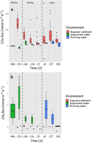
Table 2. Mixed modeling results for areal CO₂ and areal CH₄ (diffusion + ebullition) fluxes (mmol m⁻² d⁻¹): hypothesis testing for fixed factors (environment and time). df (num) is the numerator degrees of freedom for the F test for the fixed variables, df (den) displays the denominator degrees of freedom for the F test for the fixed variables, and EnvXTime represents the interaction between environment and time. Significant p-values are shown in bold.

Source		CO2				CH4
	df (num)	df (den)	F-value	p-value	df (num)	df (den)	F-value	p-value
Intercept	1	255	37.71	<0.001	1	35	164.76	<0.001
Env	2	255	13.91	<0.001	2	35	316.78	<0.001
Time	1	255	7.82	0.006	1	35	0.40	0.531
EnvXTime	2	255	8.70	<0.001	2	35	0.40	0.676

Environment (p < 0.001) but not time (p = 0.531) influenced the areal CH₄ fluxes (Table 2, Fig. 2b, Supplemental Fig. S2b). The sum of areal diffusive and ebullitive CH₄ fluxes from impounded water (1.82 [1.11] mmol m⁻² d⁻¹) were higher than areal diffusive CH₄ fluxes from exposed sediment (0.06 [0.10] mmol m⁻² d⁻¹) and lotic water (−0.96 [1.72] mmol m⁻² d⁻¹; Supplemental Table S3). Ebullition was the dominant pathway of areal CH₄ fluxes (i.e., 63% of areal diffusive + ebullitive CH₄ fluxes), whereas the shallow zone emitted 93% of areal CH₄ fluxes from impounded water (Supplemental Fig. S3).

Ecosystem CO₂ and CH₄ fluxes

The total ecosystem C flux was slightly positive (74 mol d⁻¹; day −984) or even negative (−5904 mol d⁻¹; day −233) before drawdown (i.e., when the reservoir was almost fully covered by impounded water; Fig. 3a). During reservoir drawdown, total ecosystem C fluxes were 18 718 mol d⁻¹ (day −168), 12 540 mol d⁻¹ (day −126), and 12 393 mol d⁻¹ (day −35; Fig. 3a). After reservoir drawdown, total ecosystem C fluxes were, respectively, 23 669 mol d⁻¹ (day 43), 38 713 mol d⁻¹ (day 127), and 18 568 mol d⁻¹ (day 358; Fig. 3a). On average, the total ecosystem C fluxes were −2915 mol d⁻¹ before, 14 550 mol d⁻¹ during, and 26 983 mol d⁻¹ after reservoir drawdown. Thus, ecosystem C fluxes from the reservoir were 2 and 10 times higher after than, respectively, during and before reservoir drawdown.

Figure 3. (a) Ecosystem total carbon flux, (b) carbon CO₂-eq flux, (c) ecosystem CO₂ flux, and (d) ecosystem CH₄ flux in exposed sediment, impounded water, and running water. Ecosystem CH₄ fluxes in impounded water are a sum of diffusion and ebullition but are only emitted via diffusion for exposed sediment and running water. The values below y = 0 indicate negative carbon fluxes or carbon uptake by the reservoir. Each vertical bar corresponds to a sampling campaign. The x-axis describes the 8 sampling campaigns, which are divided into 3 categories: Before (days −984 and −233), During (days −168, −126, and −35), and After (days 43, 127, and 358) reservoir drawdown. Colour version available online.

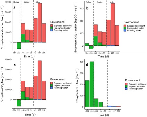
Exposed sediment contributed most of total ecosystem C fluxes, and its contribution over time followed the same temporal pattern as total ecosystem C fluxes. The mean of total ecosystem C fluxes from exposed sediment, impounded water, and lotic water was, respectively, 16 047 mol d⁻¹ (93% of total C flux), 1071 mol d⁻¹ (6%), and 154 mol d⁻¹ (1%). Thus, exposed sediment contributed most to total ecosystem C fluxes because of its high areal CO₂ fluxes and surface area, whereas lotic water had the lowest contribution to the total ecosystem C fluxes because of its small surface area.

Ecosystem CO₂ and CH₄ fluxes contributed, respectively, 99% and 1% of total ecosystem C fluxes. Ecosystem CO₂ and ecosystem CO₂-eq fluxes followed the temporal pattern of total ecosystem C fluxes in exposed sediment because this environment contributed most of total ecosystem C fluxes, and ecosystem CO₂ fluxes predominated over ecosystem CH₄ fluxes (Fig. 3b–d). By contrast, impounded water emitted 98% of ecosystem CH₄ fluxes (Fig. 3d). Thus, ecosystem CH₄ fluxes from impounded water were higher before reservoir drawdown and then decreased along DD as impounded water was replaced by exposed sediment and lotic water. Exposed sediment contributed 87%, impounded water 12%, and lotic water 1% of total C fluxes expressed in CO₂-eq (814 kg CO₂-eq d⁻¹) over a span of 100 years. The average of C flux after reservoir drawdown was 8 g CO₂-eq m⁻² d⁻¹.

Discussion

As we hypothesized, the drawdown phase of DD increased total ecosystem C (CO₂ + CH₄) fluxes from the reservoir because of higher fluxes from exposed sediment. Exposed sediment emitted, on average, 93% of the CO₂ flux and 87% of the flux expressed in CO₂-eq. At the ecosystem scale, CO₂ fluxes contributed 99% of total C fluxes while the remaining 1% was contributed by CH₄ fluxes. Most of the CH₄ fluxes (98% on average) arose from impounded water and mostly emitted via ebullition. The rates of CO₂ and CH₄ emissions from shallow impounded water were higher than from deep impounded water.

The drawdown phase of DD increased CO₂ and CH₄ fluxes from the reservoir

Before drawdown (days −984 and −233), the reservoir was a net sink of atmospheric CO₂ but a net source of CH₄. Because impounded water took more CO₂ than the CH₄ it emitted, the Enobieta Reservoir was a net sink of C before reservoir drawdown. Note that we conducted these samplings during summer, a season of high primary production in the Northern Hemisphere and therefore high CO₂ fixation via photosynthesis (Teodoru et al. 2011).

During reservoir drawdown (days −168, −126, and −35) the reservoir became a net source of C to the atmosphere, especially as CO₂. Areal CO₂ fluxes from impounded water were comparable to areal CO₂ fluxes measured elsewhere in lakes, ponds, and reservoirs (Raymond et al. 2013, Deemer et al. 2016, Holgerson and Raymond 2016). They were, however, lower than fluxes from exposed sediment and lotic water, in agreement with previous studies (Raymond et al. 2013, Kosten et al. 2018, Keller et al. 2020). Impounded waters typically emit lower areal CO₂ fluxes than lotic waters and exposed sediments because of higher CO₂ uptake by primary producers (Howard and Howard 1993, Gómez-Gener et al. 2015). C emissions from reservoirs are typically highest during their first 10–20 years, when flooded labile C is still available for microbial respiration (St. Louis et al. 2000, Barros et al. 2011). Thus, low areal CO₂ fluxes from impounded water were expected in this oligotrophic reservoir of more than 60 years of existence.

As we expected, areal CH₄ fluxes were lower in exposed sediment and lotic water than in impounded water and higher in shallow than in deep impounded water. Impounded waters are important emitters of CH₄ because of their increased anaerobic microbial functioning (Deemer et al. 2016). Methane is produced in anoxic conditions by anaerobic archaea and bacteria and emitted mainly via ebullition (Bastviken et al. 2004, Baulch et al. 2011, Deemer et al. 2016). Ebullition was the dominant pathway of CH₄ fluxes from impounded water in this study, consistent with other findings (DelSontro et al. 2016, West et al. 2016), mainly in shallow impounded water. Shallow impounded waters are hotspots for CH₄ emissions because they have a lower capacity to dissolve, trap, and oxidize CH₄. Ebullition might, however, have been underestimated because of its high spatial and temporal heterogeneity (Wik et al. 2016). Impounded water in this study emitted most of CH₄ fluxes; thus, the contribution of CH₄ to total ecosystem C fluxes decreased along reservoir drawdown as impounded water was replaced by exposed sediment.

Exposed sediments emit areal CO₂ fluxes to the atmosphere at higher rates than emissions from the water surface during the flooded periods (Catalán et al. 2014, Gómez-Gener et al. 2016, Obrador et al. 2018). Areal CO₂ fluxes from exposed sediments are higher because of their increased CO₂ diffusivity, higher microbial respiration due to higher oxic conditions, and lower CO₂ uptake by primary producers compared with inundated environments (Howard and Howard 1993, Gómez-Gener et al. 2015, Marcé et al. 2019). In this study, exposed sediment emitted most of the CO₂ fluxes within the reservoir. During the drawdown phase, these CO₂ emissions declined between days −168 and −35, likely reflecting seasonal variations in temperature and humidity. The sampling days were in October (day −126) and January (day −35), the coldest and wettest period in the study area. Lower temperature and higher humidity might have limited oxygen diffusivity, and thus microbial respiration and CO₂ production in exposed sediment, during reservoir drawdown on days −126 and −35.

After reservoir drawdown, total C fluxes at the scale of the reservoir increased and peaked on day 127, following the trend in ecosystem CO₂ fluxes. Microbial respiration, and thus CO₂ production, are higher in exposed sediments with higher content and quality of organic matter (Almeida et al. 2019, von Schiller et al. 2019, Keller et al. 2020). The areal CO₂ fluxes from exposed sediment decreased with time in this study, probably due to the reduction in quantity and quality of sediment organic C. Unfortunately, we did not assess temporal changes in the content and chemical composition of sediment organic C to support this. While the underlying mechanisms for this temporal pattern remain unclear at this stage, they provide evidence for areal emissions to be higher after than before DD.

As we assumed, areal CO₂ fluxes were lower in impounded water than areal CO₂ fluxes from exposed sediment and lotic water. However, we did not expect areal CO₂ fluxes from exposed sediment to be equal to areal CO₂ fluxes from lotic water. Lotic water, because of its high turbulence, should emit higher areal CO₂ fluxes than exposed sediment (Raymond et al. 2013, Borges et al. 2015, Gómez-Gener et al. 2015). The low pCO₂ and gas transfer velocity measured in this study might have limited emissions of CO₂ from the lotic water. We reported an average pCO₂ in lotic water of 791 μatm, nearly 4 times lower than the average pCO₂ = 3100 μatm reported from 6798 streams on a global scale (Raymond et al. 2013). In addition, the average gas transfer velocity (k₆₀₀) of 2.6 m d⁻¹ in the lotic water of this study is lower than the mean of k₆₀₀ values = 45.0 m d⁻¹ reported in a review on gas exchanges in streams (Ulseth et al. 2019).

Carbon dioxide and CH₄ contributed on average 99% and 1% of total ecosystem C fluxes, respectively. Expressed in CO₂-eq, the contribution of CH₄ rose to 6% of total ecosystem C fluxes because of the higher global warming potential of CH₄ compared to CO₂ (IPCC 2013). Ecosystem CH₄ fluxes are responsible for ∼60%–79% of CO₂-eq from surface waters of lakes, ponds, and reservoirs (Deemer et al. 2016, DelSontro et al. 2016, van Bergen et al. 2019), whereas exposed sediments are poor emitters of CH₄ because of their increased aerobic conditions (Obrador et al. 2018, Marcé et al. 2019, Arce et al. 2021, Paranaíba et al. 2021). Impounded water emitted 98% of CH₄ fluxes while the remaining 2% was contributed by the combined exposed sediment and lotic water. Although exposed sediment occupied a large surface area, its contribution to ecosystem CH₄ fluxes was low because of its low areal CH₄ fluxes. The contribution of lotic water to ecosystem CH₄ fluxes was low because it occupied a negligible surface area.

Conclusion: implication of dam decommissioning for the carbon footprint of the reservoir and future perspectives

The average ecosystem flux in CO₂-eq after reservoir drawdown was 8 g CO₂-eq m⁻² d⁻¹, slightly higher than the flux reported on a global scale in surface waters of reservoirs between 4.25 g CO₂-eq m⁻² d⁻¹ (St. Louis et al. 2000) and 6.64 g CO₂-eq m⁻² d⁻¹ (Deemer et al. 2016). The flux reported in this study is also higher than the flux from hydroelectric reservoirs worldwide; 2.55–7.64 g CO₂-eq m⁻² d⁻¹ (Deemer et al. 2016). Hydropower was considered a green source of energy, but GHG emissions from reservoirs contribute to the global C budgets (Deemer et al. 2016, St. Louis et al. 2000, Barros et al. 2011) even before considering their C emissions during and after DD. The high CO₂ fluxes from exposed sediment reported in this study indicate the importance of the drawdown phase of DD as a hot moment for CO₂ and CH₄ emissions from a reservoir. Thus, the exclusion of GHGs related to the end-of-life of dams may result in an underestimation of the C footprint of reservoirs.

The decrease in CO₂ fluxes in exposed sediment may be a seasonally specific feature that warrants further investigation beyond the short-term duration of this study. Furthermore, exposed sediments are amenable environments for vegetation growth, which may overturn the effects of DD on the C emissions of a reservoir by fixing atmospheric CO₂. However, we lack empirical evidence to clarify the role of plant regrowth in the C dynamics in reservoirs following DD. Thus, we emphasize a need to know the drivers of CO₂ fluxes from exposed sediments and mid- and long-term effects of DD on C emissions in reservoirs, including the role of plant recolonization, and to include DD in the C footprint of reservoirs. To conclude, this study sets a baseline for promising future studies to improve our understanding of how the C dynamics of reservoirs are affected by dam decommissioning.

Acknowledgements

We acknowledge M. Koschorreck and M. Badia who helped in sampling activities.

Disclosure statement

No potential conflict of interest was reported by the author(s).

Additional information

Funding

This study was funded by the projects Alteration of carbon sinks and sources in shrinking inland waters (Alter-C), the Spanish Ministry of Science, Innovation and Universities (refs: PID2020-114024GB-C31 funded by MCIN/AEI /10.13039/501100011033/) and Effects of the drawdown of Enobieta Reservoir (Navarre) on the biodiversity and functioning of river ecosystems (DESEMBALSE), Foundation BBVA (ref: PI064-17). AM was supported by an FI grant from the Agència de Gestió d’Ajuts Universitaris i de Recerca (AGAUR) of the Generalitat de Catalunya. DvS and BO acknowledge support through the Consolidated Research Group 2017SGR0976. RM acknowledges support by the Generalitat de Catalunya through the Consolidated Research Group 2017SGR1124, and by the CERCA program. AE and MA support of the Basque Government through the Consolidated Research Group IT951-16. AM got a predoctoral grant by the University of the Basque Country (UPV/EHU). DvS is a Serra Húnter Fellow.

References

- Almeida RM, Paranaíba JR, Barbosa Í, Sobek S, Kosten S, Linkhorst A, Mendonça R, Quadra G, Roland F, Barros N. 2019. Carbon dioxide emission from drawdown areas of a Brazilian reservoir is linked to surrounding land cover. Aquat Sci. 81:1–9.
- Arce MI, Bengtsson MM, von Schiller D, Zak D, Täumer J, Urich T, Singer G. 2021. Desiccation time and rainfall control gaseous carbon fluxes in an intermittent stream. Biogeochemistry. 155:381–400.
- Barros N, Cole JJ, Tranvik LJ, Prairie YT, Bastviken D, Huszar VLM, del Giogio P, Roland F. 2011. Carbon emission from hydroelectric reservoirs linked to reservoir age and latitude. Nat Geosci. 4:593–596.
- Bastviken D, Cole J, Pace M, Tranvik L. 2004. Methane emissions from lakes: dependence of lake characteristics, two regional assessments, and a global estimate. Global Biogeochem Cy. 18:1–12.
- Baulch HM, Dillon PJ, Maranger R, Schiff SL. 2011. Diffusive and ebullitive transport of methane and nitrous oxide from streams: Are bubble-mediated fluxes important? J Geophys Res. 116:G04028.
- Bednarek AT. 2001. Undamming rivers: a review of the ecological impacts of dam removal. Environ Manage. 27:803–814.
- Bellmore JR, States U, Pess GR, Duda JJ, O’Connor JE, East AE, Foley MM, Wilcox AC, Major JJ, Shafroth PB, et al. 2019. Conceptualizing ecological responses to dam removal: if you remove it, what’s to come? Bioscience. 69:26–39.
- Borges AV, Darchambeau F, Teodoru CR, Marwick TR, Tamooh F, Geeraert N, Omengo FO, Guérin F, Lambert T, Morana C, et al. 2015. Globally significant greenhouse-gas emissions from African inland waters. Nat Geosci. 8:637–642.
- Catalán N, von Schiller D, Marcé R, Koschorreck M, Gomez-Gener L, Obrador B. 2014. Carbon dioxide efflux during the flooding phase of temporary ponds. Limnetica. 33:349–360.
- Crusius J, Wanninkhof R. 2003. Gas transfer velocities measured at low wind speed over a lake. Limnol Oceanogr. 48:1010–1017.
- Deemer BR, Harrison JA, Li S, Beaulieu JJ, DelSopntro T, Barros N, Bezerra-Neto JF, Powers SM, Dos Santos MA, Arie Vonk J. 2016. Greenhouse gas emissions from reservoir water surfaces: a new global synthesis. Bioscience. 66:949–964.
- DelSontro T, Boutet L, St-Pierre A, del Giorgio PA, Prairie YT. 2016. Methane ebullition and diffusion from northern ponds and lakes regulated by the interaction between temperature and system productivity. Limnol Oceanogr. 61:S62–S77.
- DelSontro T, Mcginnis DF, Sobek S, Ostrovvsky I, Wehrli B. 2010. Extreme methane emissions from a Swiss hydropower reservoir: contribution from bubbling sediments. Environ Sci Technol. 44:2419–2425.
- Deshmukh C, Guérin F, Vongkhamsao A, Pighini S, Oudone P, Sopraseuth S, Godon A, Rode W, Guédant P, Oliva P, et al. 2018. Carbon dioxide emissions from the flat bottom and shallow Nam Theun 2 Reservoir: drawdown area as a neglected pathway to the atmosphere. Biogeosciences. 15:1775–1794.
- Downing JA, Cole JJ, Middelburg JJ, Striegl RG, Duarte CM, Kortelainen P, Prairie YT, Laube KA. 2008. Sediment organic carbon burial in agriculturally eutrophic impoundments over the last century. Global Biogeochem Cy. 22:1–10.
- Doyle MW, Stanley EH, Harbor JM, Grant GS. 2003. Dam removal in the United States: emerging needs for science and policy. EOS. 84:29–36.
- Frankignoulle M. 1988. Field measurements of air-sea CO2 exchange. Limnol Oceanogr. 33:313–322.
- Fromin N, Pinay G, Montuelle B, Landais D, Ourcival JM, Joffre R, Lensi R. 2010. Impact of seasonal sediment desiccation and rewetting on microbial processes involved in greenhouse gas emissions. Ecohydrology. 3:339–348.
- Gobierno de Navarra. 2019. Ficha climática de la estación—Meteo Navarra.es [Climatic data of the meteo-station Navarre]. http://meteo.navarra.es/climatologia/fichasclimaticas_estacion.cfm?IDestacion=74. Spanish.
- Gómez-Gener L, Obrador B, von Schiller D, Marcé R, Casas-Ruiz JP, Proia L, Acuña V, Catalán N, Muñoz I, Koschorreck M. 2015. Hot spots for carbon emissions from Mediterranean fluvial networks during summer drought. Biogeochemistry. 125:409–426.
- Gómez-Gener L, Obrador B, Marcé R, Acuña V, Catalán N, Casas-Ruiz JP, Sabater S, Muñoz I, von Schiller D. 2016. When water vanishes: magnitude and regulation of carbon dioxide emissions from dry temporary streams. Ecosystems. 19:710–723.
- Gordon ND, McMahon TA, Finlayson BL, Gippel CJ, Nathan RJ, Knight S, editors. 2004. Stream hydrology. An introduction for the ecologists. 2nd ed. Chichester (UK): Wiley and Sons Ltd.
- Harrison JA, Deemer BR, Birch MK, Malley MTO. 2017. Reservoir water-level drawdowns accelerate and amplify methane emission. Environ Sci Technol. 51:1267–1277.
- Holgerson MA, Raymond PA. 2016. Large contribution to inland water CO2 and CH4 emissions from very small ponds. Nat Geosci. 9:222–226.
- Howard DM, Howard PJA. 1993. Relationships between CO2 revolution, moisture content, and temperature for a range of soil types. Soil Biol Biochem. 25:1537–1546.
- [IPCC] Intergovernmental Panel on Climate Change. 2013. Summary for policymakers. In: Stocker TF, Qin G–K, Plattner M, Tignor SK, Allen J, editors. Climate change 2013: the physical science basis. Contribution of work group I to the fifth assessment report on the Intergovernmental Panel on Climate Change.
- [IPCC] Intergovernmental Panel on Climate Change. 2019. Refinement to the 2006 IPCC guidelines for national greenhouse gas inventories. Volume 4 [accessed 2019 December 24]. https://www.ipcc-nggip.iges.or.jp/public/2019rf/index.html
- Jin H, Yoon TK, Lee SH, Im J, Park JH. 2016. Enhanced greenhouse gas emission from exposed sediments along a hydroelectric reservoir during an extreme drought event. Environ Res Lett. 11:124003.
- Keller PS, Catalán N, von Schiller D, Grossart HP, Koschorreck M, Obrador B, Frassl MA, Karakaya N, Barros N, Howitt JA, et al. 2020. Global CO2 emissions from dry inland waters share common drivers across ecosystems. Nat Commun. 11:1–8.
- Keller PS, Marcé R, Obrador B, Koschorreck M. 2021. Global carbon budget of reservoirs is overturned by the quantification of drawdown areas. Nat Geosci. 14:402–408.
- Kosten S, van den Berg S, Mendonça R, Paranaíba JR, Roland F, Sobek S, Van Den Hoek J, Barros N. 2018. Extreme drought boosts CO2 and CH4 emissions from reservoir drawdown areas. Inland Waters. 8(3):329–340.
- Larrañaga A, Atristain M, von Schiller D, Elosegi A. 2019. Environmental diagnosis of the river network prior to the dismantling of a dam and preliminary results of the emptying effects of Enobieta. Navarre Ingeniería Civil. 193:1–12.
- Li M, Peng C, Zhu Q, Zhou X, Yang G, Song X, Zhang K. 2020. The significant contribution of lake depth in regulating global lake diffusive methane emissions. Water Res. 590:115465.
- Maathuis BHP, Wang L. 2006. Digital elevation model based hydro-processing. Hong Kong: Geocarto International Center. 1.
- Madsen H, Thyregod P. 2010. Introduction to general and generalized linear models. Boca Raton (FL): CRC Press.
- Marcé R, Obrador B, Gómez-Gener L, Catalán N, Koschorreck M, Arce MI, Singer G, von Schiller D. 2019. Emissions from dry inland waters are a blind spot in the global carbon cycle. Earth-Sci Rev. 188:240–248.
- Marks JC, Haden GA, O’Neill M, Pace C. 2010. Effects of flow restoration and exotic species removal on recovery of native fish: lessons from a dam decommissioning. Restor Ecol. 18:934–943.
- Mendonça R, Müller RA, Clow D, Verpoorter C, Raymond P, Tranvik L, Sobek S. 2017. Organic carbon burial in global lakes and reservoirs. Nat Commun. 8:1694.
- Miranda E, Mutiara AB, Wibowo WC. 2018. Classification of land cover from Sentinel-2 imagery using supervised classification technique (preliminary study). 2018 international conference on information management and technology (ICIMTech). IEEE; p. 69–74.
- Obrador B, von Schiller D, Marcé R, Gómez-Gener L, Koschorreck M, Borrego C, Catalán N. 2018. Dry habitats sustain high CO2 emissions from temporary ponds across seasons. Sci Rep. 8:3015.
- Pacca S. 2007. Impacts from decommissioning of hydroelectric dams: a life cycle perspective. Climate Change. 84:281–294.
- Paranaíba JR, Aben R, Barros N, Quadra G, Linkhorst A, Amado AM, Brothers S, Catalán N, Condon J, Finlayson CM, et al. 2021. Cross-continental importance of CH4 emissions from dry inland-waters. Sci Total Environ. 814:151925.
- Perera D, Smakhtin V, Williams S, North T, Curry A. 2021. Ageing water storage infrastructure: an emerging global risk. In: UNU-INWEH Report Series; Hamilton (ON): United Nations University-Institute for Water, Environment and Health (UNU-INWEH). ISBN:978-92-808-6105-1.
- Pinheiro J, Bates D. 2018. nlme: linear and nonlinear mixed effects models, R package version 3.1–137.
- Pinheiro JC, Bates DM. 2000. Mixed effects models in S and S-Plus, 3rd ed. New York (NY): Springer.
- R Core Team. 2021. R: a language and environment for statistical computing. R Foundation for statistical computing, Vienna. http://www.R-project.org/
- Rathore R, Kumar V, Ranjan A, Tiwari S, Goswami A, Agwan M. 2018. Extraction of watershed characteristics using GIS and digital elevation model. Int J Res Eng. 1:62–65.
- Raymond PA, Hartmann J, Lauerwald R, Sobek S, McDonald C, Hoover M, Butman D, Striegl R, Mayorga E, Humborg C, et al. 2013. Global carbon dioxide emissions from inland waters. Nature. 503:355–359.
- St. Louis VL, Kelly CA, Duchemin E, Rudd JWM, Rosenberg DM. 2000. Measuring fluxes of greenhouse gases from reservoir surfaces. Bioscience. 50:766–775.
- Stanley EH, Casson NJ, Crawford JT, Loken LC, Oliver SK. 2016. The ecology of methane in streams and rivers: patterns, controls and global significance. Ecol Monogr. 86:146–171.
- Stanley EH, Doyle MW. 2003. Trading off: the ecological effects of dam removal. Front Ecol Environ. 3220:15–22.
- Teodoru CR, Prairie YT, del Giorgio PA. 2011. Spatial heterogeneity of surface CO2 fluxes in a newly created Eastmain-1 reservoir in northern Quebec, Canada. Ecosystems. 14:28–46.
- Ulseth AJ, Hall RO, Boix Canadell M, Madinger HL, Niayifar A, Battin TJ. 2019. Distinct air–water gas exchange regimes in low- and high-energy streams. Nat Geosci. 12:259–263.
- van Bergen TJHM, Barros N, Mendonça R, Aben RCH, Althuizen IHJ, Huszar V, Lamers LPM, Lürling M, Roland F, Kosten S. 2019. Seasonal and diel variation in greenhouse gas emissions from an urban pond and its major drivers. Limnol Oceanogr. 64:2129–2139.
- von Schiller D, Datry T, Corti R, Foulquier A, Tockner K, Marcé R, García-Baquero OI, Obrador B, Elosegi R, et al. 2019. Sediment respiration pulses in intermittent rivers and ephemeral streams. Global Biogeochem Cy. 33:1251–1263.
- West WE, Creamer KP, Jones SE. 2016. Productivity and depth regulate lake contributions to atmospheric methane. Limnol Oceanogr. 61:S51–S61.
- Wik M, Thornton BF, Bastviken D, Uhlbäck J, Crill PM. 2016. Biased sampling methane release from northern lakes: a problem of extrapolation. Geophys Res Let. 43:1256–1262.
- Yang M, Geng X, Grace J, Lu C, Zhu Y, Zhou Y, Lei G. 2014. Spatial and seasonal CH4 flux in the littoral zone of Miyun Reservoir near Beijing: the effects of water level and fluctuation. PLoS One. 9:e94275.