Optimal stowage on Ro-Ro decks for efficiency and safety

ABSTRACT

The roll-on/roll-off (Ro-Ro) ships are true workhorses of coastal and deep-sea shipping. They are valued for their versatility to transport heterogeneous cargo and short turnaround times in ports. However, the optimal utilisation of cargo space has been inherently problematic with the Ro-Ro concept. In view of the existing attempts to contrive optimal stowage plans, the paper proposes three practical improvements with respect to the state of the art. The improvements lead to a finer approach to ship stability, fire safety, and cargo handling efficiency when optimising cargo stowage on Ro-Ro decks. Formally, we express the stowage problem as a mixed-integer linear programming (MILP) problem and solve it to optimality. The paper outlines the mathematical formulation, provides a numerical example, and studies practical application aspects.

1. Introduction

The Ro-Ro ships transport a wide variety of wheeled cargo such as private cars, buses, vans, semi-trailers, project cargo, as well as thousands of passengers on coastal ferry voyages. The wheeled cargo autonomously rolls on/off the ship through ramps, as opposed to being handled with specialised and costly equipment (e.g. cranes used for container ships). One shortcoming of the Ro-Ro concept is its inherent difficulty to utilise the cargo space efficiently. The presence of heterogeneous cargo in size and type makes it difficult to optimise the stowage plan, which aims to maximise the net revenue per time unit by loading as much cargo as possible (Jansson and Shneerson 1987), subject to stability and other constraints. If there is a possibility to choose which cargo load, the selection process will maximise the net revenue by picking the most profitable subset of cargo. If a stowage plan is suboptimal, precious revenues will be lost and safety jeopardised. And as the maritime industry is undergoing digitalisation with various onboard decision support systems becoming standard, the optimal stowage problem has attracted attention in the area of operational research (OR) (Øvstebø et al. 2011; Øvstebø et al. 2011; Wathne 2012; Hansen et al. 2016; Mulder and Dekker 2016; Parreño et al. 2016; Seixas et al. 2016).

1.1. Work so far

In Ro-Ro applications the work is represented by Øvstebø et al. (2011a), Øvstebø et al. (2011b), Wathne (2012), and Hansen et al. (2016). The proposed approaches provide a solid basis for solving the Ro-Ro ship stowage problem, given its peculiarities compared to stowage problems on other ships (e.g. container ships). In addition to the description of a mixed-integer linear programming (MILP) model, the attention is given to alternative solution methods such as Tabu Search and genetic algorithms. However, these approaches have a number of challenges, as discussed later.

Other related work comes from applications to general or specialised cargo such as container ships. Thus, Tang et al. modelled the ship stowage planning problem of steel coils stacked in two layers and carried on cargo ships (2015). The objective was to determine the location of variable size coils of steel on the ship, subject to ship stability and cargo handling efficiency. Seixas et al. (2016) worked on an optimal two-dimensional stowage of heterogeneous cargo on a single deck, supply vessels to offshore rigs. The vessel would visit several offshore rigs during a return voyage, aiming to maximise the deck area utilisation and value of cargo load, subject to safety and other constraints. Although the adopted discretisation and solution methods may be appropriate for single deck, small to medium size vessels, they are computationally prohibitive for Ro-Ro ships with significantly larger deck areas, multiple decks, and a wider variety of cargo types.

The cargo stowage problem on container ships has the most developed theory and applications (Avriel and Penn 1993; Wilson and Roach 1999; Wilson and Roach 2000; Pacino et al. 2011; Pacino et al. 2012; Ding and Chou 2015; Parreño et al. 2016). The problem concerns the optimal placement of containers into cargo holds by cranes, so that the utilisation of payload capacity is maximised and sequential cargo handling within a multi-port journey is most efficient. Obviously, stowage, ship stability, strength and other constraints have to be respected. The cargo space is discretised into equal size cells with the capacity of two TEUs (Twenty-Foot Equivalent Units), i.e. they can stow two 20′ or one 40′ (or 45′) long container, which are considered standard. The problem is typically formulated as a linear integer programming, and sometimes as a binary liner problem (Avriel and Penn 1993). As pointed out by Ding and Chou. (2015), the binary formulation leads to a large number of variables and constraints, which can be impractical for the container stowage problem. The adopted discretisation approach benefits from the fact there are standard container sizes, and there are only a few of them. This is not the case for Ro-Ro ships, where the variety of cargo sizes is unregulated. This makes their mathematical models obviously different.

1.2. Addressed challenges

1.2.1. Discretisation

The proposed discretisation approaches in the literature are deficient. The first approach discretises the deck area into lanes or rectangular slots designating alternative cargo locations. The size of the lanes and slots is, however, unknown in advance and used as a bounded decision variable to be settled during the optimisation (Øvstebø et al. 2011; Wathne 2012). Consequently, some resultant layouts can appear unrealistic. Because of the unknown slot size, the imposed intact stability constraints are evaluated based on predicted rather than on actual values. This necessitates a verification of optimisation results against stability requirements, and the results might not pass the test. In the second approach, cargo slots are determined by merging neighbouring cells of a regular gird (Hansen et al. 2016). However, the cell size needs to be predetermined in advance by the user, seeking a balance between the result accuracy and time efficiency. The presented model was applied to a single deck scenario only.

We propose to work around these difficulties by creating individual grids for each cargo type on those decks where this cargo can be stowed (Section 2.1). The grids can be rectangular or of any other type, with the cells size (i.e. the slot size) corresponding to the size of cargo (e.g. a private car or semi-trailer) augmented by the necessary passage clearance on each side. There is also complete certainty about the grid resolution, as the grid cells always reflect the corresponding cargo size.

1.2.2. Fire safety

Being large subdivided spaces, Ro-Ro decks are notoriously known to introduce safety vulnerabilities. A recent FIRESAFE study by European Maritime Safety Agency (EMSA) found that some 30% of fires have happened on Ro-Ro decks (Wikman 2016). These fires have been mainly electrical, originating within vehicles themselves – predominantly in electric cars and other alternative-fuel vehicles (AFV)¹ – or in reefer containers. A commonly agreed strategy to reduce the fire risk is to ensure early detection, confirmation, and suppression of fires (Siewers and Tosseviken 2016). This can be achieved by controlling the cargo distribution on decks, thereby securing the required performance of automatic fire suppression as well as easy access to vehicles by the crew. For instance, an uncontrolled arrangement of large vehicles such as semi-trailers, which could not be easily moved out of the way, has blocked access to ignitions sources and inhibited firefighting in the past (Ware 2017). The ceiling-based drenchers have proven ineffective due to shielding of water distribution by high cargo (trucks, trailers, semi-trailers, etc.) (Wikman 2016).

Despite the unequivocal link between the cargo stowage planning and fire safety, it has been overlooked in the literature. This paper bridges this gap by developing and incorporating the corresponding safety constraints into the optimal stowage plan (Section 2.2). Additionally, we examine the effect of the introduced constraints on the net revenue being maximised.

1.2.3. Minimal turnaround

The proposed solution to the time efficient cargo loading and unloading has a common pitfall. As a Ro-Ro ship visits en route several ports of call, the cargo that continues the journey to next ports and is shifted to other locations to free the way for other cargo being discharged or loaded. As this operation increases time in port, it is addressed by penalising the blocking cargo through the assignment of shifting cost proportional to the cargo size, its relative location, and shifting distance. The assumption is that during the optimisation such cargo will be assigned to different locations where the shifting cost is lower or nil. However, this approach does guarantee an optimal stowage plan with zero shifting cost. In practice, the obstruction of unloading or loading operations even by one vehicle can be unacceptable, especially if this vehicle is a semi-trailer or alike.

This paper offers a different approach that eliminates any need for shifting cargo at all, ensuring zero shifting cost for an optimal stowage plan (Section 2.3).

1.3. Paper organisation

The offered improvements are detailed in Section 2, followed by a mathematical formulation of the refined stowage problem (Section 3) and its example application (Section 4). Section 5 examines the effect of the introduced safety constraints, if they were used in real applications, on the maximised revenue and computation time. Section 6 concludes the paper.

2. The proposed improvements

2.1. Improvement 1: discretisation of stowage locations

The mathematical formulation of optimal stowage planning is driven by a discretisation approach for locations of heterogeneous cargo on decks. In our work, we assign individual grids for each cargo type on those decks where this cargo can be stowed. The grids are sized to deck dimensions and the number of grids corresponds to the number of cargo types, which can be stowed on a given deck. That is, each cargo type is associated with an individual grid of which copy is assigned to each deck, except those decks where the cargo cannot be stowed on. For example, if only cars and semi-trailers were transported and they could be stowed on two decks, each deck would be associated with two grids, resulting in four grids in total.

The grids can be regular or irregular, with the cells size corresponding to the size of cargo augmented by the necessary passage clearance on each side. When vehicles are always stowed along the X-axis (the centre line), then regular grids can be used (Figure 1). Irregular girds are used when vehicles can be aligned with the sidewalls – as opposed to the centre line – to better utilise the deck area. For example, this can be the case towards the fore of the ship where the deck area gets gradually narrower. It is important to note that the choice of the grid type, i.e. regular or irregular, does not affect the mathematical formulation.

Figure 1. Two example regular grids for large (lower grid) and smaller cargo units.

If cargo is not required to be aligned with deck lanes (may not exist at all on small ferries), the cell size of an associated regular grid would then correspond to the actual dimensions of the cargo, adding side clearances for opening doors, passage etc. In case when the decks are divided into longitudinal lanes and the vehicles must be stowed on those lanes, the width of a regular grid cell is simply sized to match the lane width.

Figure 2 shows an example grid laid (in blue) over a deck. Each cell represents an alternative location of corresponding cargo type on the deck. During the optimisation, the grid cells are associated with binary decision variables (=1 cell has cargo or = 0 when has not) of which optimal values are sought. Before the optimisation, the grid is pre-processed by excluding the cells that overlap or intersect with the areas where the stowage is physically impossible or prohibited, as shown in Figure 2. There could also be areas of special purpose (e.g. only dangerous goods or high-risk cargo can be stowed) or being of different attributes to the main deck area (e.g. different max loading capacity).

Figure 2. An example grid laid over the main deck (deck 3), excluding areas (marked) where the stowage is impossible (e.g. central and side casings, ramps, etc.) or prohibited (e.g. areas designed for other cargo, necessary clearances for safety reasons). There are also designated areas of special purpose (e.g. only specific cargo type can be stowed there).

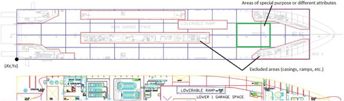
Due to the use of an individual grid for each cargo type, the cargo location is precisely known. This leads to accurate ship stability, strength, determination of geometric overlap with deck features (e.g. pillars, excluded areas from stowage) and other calculations. This algorithmic feature is also helpful in determining the overlap between cargo units of different types, i.e. the overlap between cells belonging to different grids (Figure 1(b)), as the deck area is shared (Figure 1(b)). This overlap is then eliminated by imposing inequality constraints (Section 3.5).

2.2. Improvement 2: fire safety

The stowage planning has to take into account the fire risk. The FIRESAFE study has proposed several risk control measures (Wikman 2016) that can be incorporated into the optimal stowage plan, as listed in Table 1.

Table 1. List of risk control measures (RCM) proposed in FIRESAFE study (Wikman 2016).

#	RCM description	Ref. in study
1	Loading/Storage of cargo/vehicles as per their specific risk.	S5
2	A policy on reefer units needs to be available. If accepted on board, they should be placed in dedicated areas (weather decks when possible, and preferably an area covered by CCTV). Power transfer cables should be in good condition, replaced frequently and only handled by the designated crew. Reefer units of dubious quality should be rejected. Stowage area should be checked frequently during the voyage.	E38
3	Grouping of reefer units to better manage controls (in the stern could be most practicable).	E34
4	Putting reefer units along the ship sides to simplify inspections and connections.	E35
5	Increased deck height.	S45
6	Loading procedure where high cargo (trucks/trailers) are mixed with low cargo (cars).	S46
7	Mandatory spacing of at least 60 cm between every four vehicles (to facilitate fire patrol and extinguishment).	S48
8	Special areas – Passive separation. Partition could prevent smaller fires from spreading over the entire deck, which may result in a loss of the ship. As the partition may limit the usability of the cargo deck only a dedicated and limited area is envisaged to be separated. Especially HEV, BEV, FC vehicles and vehicles with refrigerating units shall be stored in this area. Mobile partition like roller shutter or sliding doors as well as fixed insulated walls may realize suitable protected to adjacent areas.	S52
9	Special areas - Water wall. This risk control option pursues the same objective as the mobile or fixed partition of the cargo deck. Instead of a solid structure a water wall is intended to be used to separate the cargo hold.	S53
10	Water wall sections concept in enclosed ro-ro spaces. Water wall system advantages: loading/unloading sequences not impaired by water wall system equipment, convection cells limited by transverse bounds created by water wall system, fire containment enhanced, smoke containment allowing fire-fighting team to tackle the fire, and retrofit opportunity.	S56

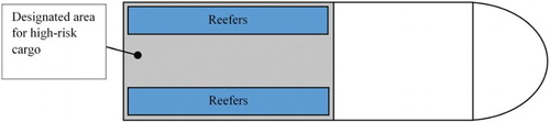
The measures 3–7 are explicitly incorporated in the stowage planning in our work, whereas measures 1 and 2 are implicit. The measures 8–10 are not addressed, as they require changes to deck design and hence are beyond this paper’s scope. The implicit measure 1 alludes to risk profiling of loaded cargo, which can be done automatically from vehicle number plates, declarations or by other means. The risk profiling is not addressed in our work. The measure 2 is a direct consequence of risk profiling, limiting the stowage of reefers, and other high-risk cargo such as electric cars, to a designated area (Figure 2). Further, the measures 3 and 4 suggest such a designated area should be in the stern where reefers are aligned along the ship sides for simpler inspection and connection to electrical sockets. Figure 3 illustrates the arrangement of reefers on deck, where the corresponding constraints are introduced in Section 3.5.

Figure 3. Arrangement of reefers (high-risk cargo) on deck.

The measure 5 is aimed at ensuring the effectiveness of the drencher system, which has been shown to become ineffective due to shielding of water distribution by high cargo (trucks, trailers, semi-trailers, etc.) (Wikman 2016). The measure 5 should naturally be considered during design. But since an increase in the deck height is to potentially undermine ship’s stability and payload capacity, demonstrating its cost-effectiveness might be problematic. Alternatively, the measure can be imposed during the stowage planning by controlling the minimal headroom. The measure 6 requires mixing high and low cargo, which would primarily lead to larger average headroom and hence better effectiveness of the drencher system. Thus, measures 5 and 6 are akin in purpose and can be combined together by imposing a constraint on the average headroom on the deck (Section 3.5).

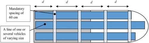
The measure 7 suggests the mandatory spacing of 60 cm between every four vehicles. This applies longitudinally and transversely. We implement this requirement by introducing the longitudinal spacing at equal distance d, across the entire deck breadth, as shown in Figure 4.

Figure 4. Longitudinal spacing of at least 60 cm every D meters, to facilitate fire patrol and extinguishment.

The above requirements would indirectly address the experience with other high-risk cargo (e.g. electric cars). Thus in some fire accidents, the access for effective firefighting was greatly limited by large vehicles such as semi-trailers that could not be swiftly moved out of the way (Ware 2017). By positioning the high-risk cargo in the stern on designated areas and introducing the mandatory spacing between vehicles, the access for firefighters would significantly be improved.

2.3. Improvement 3: loading and unloading

It is assumed that the itinerary, schedule, and ship capacity are fixed, shifting the focus to the operational planning problem of optimally distributing cargo onboard (Christiansen et al. 2007). An itinerary includes several ports of call visited sequentially. In each port, cargo is loaded and unloaded and the ship may simultaneously transport cargo to be unloaded in different ports. Figure 5 demonstrates an example itinerary with six types of cargo loaded and unloaded in six different ports. Thus, cargo 1 is loaded in port 1 and unloaded in port 6, i.e. it has to be transported along the entire itinerary. Other cargo types are transported between fewer ports. Stowage of cargo 1 will need to be coordinated with all other cargo types, whereas by port 3, cargo 2 and cargo 3 will be unloaded, having no effect on stowage planning of later loaded cargo types. Hence, an itinerary can be split into five cargo-loading conditions that are physically independent but logistically linked. The cargo included in several loading conditions is referred to as continuing cargo. Each loading condition is assumed independent in ship stability and other physical constraints to be satisfied. However, due to the presence of continuing cargo, integrity constraints have to be imposed across affected loading conditions.

Figure 5. Example itinerary consisting of five loading conditions.

Securing a swift loading and unloading in ports is the key prerequisite for an optimal stowage plan. To achieve that, stowage locations should be assigned in such a way so that the continuing cargo does not impede neither loading nor unloading. The earlier described discretisation method (Section 2.1) enables two approaches:

1. Assignment of penalty to minimise the impeding continuous cargo (analogous used in the literature);

2. Elimination of impeding cargo from a loading/un-loading path altogether.

The penalty cost is proportional to the shortest path to a corresponding exit ramp. Given the cargo location, the shortest path is determined to the exit ramp on the actual deck and then to the exit on the main deck (Figure 6). The shortest path is determined using the A* search algorithm (Hart et al. 1968).

Figure 6. Illustration of the shortest path on two decks.

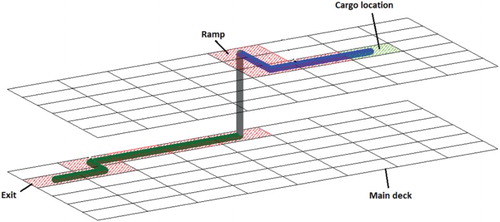
To eliminate the impeding continuing cargo, we find the shortest path for each cargo unit towards a given exit ramp, identify continuing cargos stowed on this path, and introduce a set of inequality constraints to guarantee the absence of continuing cargos on the path; (Section 3.5) outlines these constraints. We also consider two application cases:

1. Continuing cargo is stowed in the same location throughout the itinerary;

2. The location of continuing cargo is adjusted in each port to better utilise deck area, in view of new cargo being loaded.

Switching between the two options is done by activating corresponding constraints (Section 3.5).

3. Mixed-integer linear programming model

3.1. Indices

Table

l	loading condition
d	deck
g	grid
c	grid cell

3.2. Sets

Table

$L$	set of loading conditions
$D$	set of decks
$G_d$	subset of grids (cargoes) on deck d
$C_g$	subset of grid cells associated with grid g
$P$	set of all hoistable panels (decks)
$P_d$	subset of panels above deck d
$C_p$	subset of all grid cells on panel p
$P_{dgc}$	subset of panels that are above grid cell c of type g on deck d
H	set of cargo heights

3.3. Parameters

Table

${\kappa }_{ldgc}=k\cdot d_{ldgc}^{\ast }$	cost associated with cargo type g at deck d and grid cell c and in the loading condition l, and k is some scaling factor making sure that $\left({\pi }_g-{\kappa }_{ldgc}\right)>0$.
$d_{ldgc}^{\ast }$	shortest distance from cell c to the exit ramp
${\pi }_g$	revenue per cargo unit of type g (or of grid index g). The revenue is kept fixed during calculations, whereas the cost depends on the cargo location.
$N_g$	number of cargo units of type g (or grid g)
$W_g$	individual weight of cargo unit of type g (corresponds to the grid index g)
$W_d^{max}$	maximal allowable weight of cargo on deck d
$p_g$	individual floor pressure (maximal among all contract surfaces) due to the weight of cargo unit of type g (corresponds to the grid index g)
$P_g^{max}$	maximal allowable floor pressure within grid cell g
$h_g$	height of the cargo type g
$H{C}_d$	deck ceiling height
$\delta$	required minimal clearance below the ceiling
$H_{dpc}$	height of panel p with grid cell c relative to deck d’s floor
$M_r$	roll moment
$M_t$	trim moment
$b_c$	width (transversely) of grid cell g
${\delta }_g^y$, ${\delta }_g^x$	transverse and longitudinal clearances around cargo of type g, respectively
$LC{G}_g$	longitudinal centre of gravity (from the side of the loading/unloading ramp) of cargo unit of type g. This value is almost certain when the cargo units roll on and park facing the same direction. Otherwise, when the direction can be changed, the value becomes uncertain
$\left(X_d^0,Y_d^0\right)$	origin of the deck’s d coordinate system (left bottom point) with respect to the global coordinate system (see Figure 2 and Figure 7)
$\left(X_d^c,Y_d^c\right)$	coordinates of CoG of deck d with respect to the global coordinate system
$M_r^{max}$	max roll moment around the centre line
$M_t^{max}$	max trim moment around the midship
$H_d$	height of the deck d from the keel
$VC{G}_g$	vertical centre of gravity of cargo unit of type g
$LWT$	lightweight of the ship
$VCG$	updated vertical centre of gravity of lightweight ship
$VC{G}_0$	vertical centre of gravity of lightweight ship
$A_p$	area of panel p
$w_p$	unit area weight of panel p
$Z_{min},Z_{max}$	Limiting VCG values
U	upper limit for the average headroom per deck and it is calculated as the average between the maximal and second maximal height of the stowed cargos: $U=\frac{maxH+max{H}_1}{2}\text{ where }{H}_1=H\mathrm{\setminus }\left\{maxH\right\}$

3.4. Decision variables

Table

$x_{ldgc}$	binary decision variable, and if $x_{ldgc}$= 1 then cargo is in loading condition l, stowed on deck d, its corresponding grid g, and within specific grid’s cell c. The actual number of binary decision variables per cargo type scales as $\left|L\right|\times \left|D\right|\times \left|G_d\right|\times |C_d|$. Thus, $x_{ldgc}$ corresponds to a cell address.
$H_p$	relative heights of hoistable panels (decks) with respect to the main deck floor, $p\in P$.

3.5. The model

(1) $\sum _l^{|L|}\sum _d^{|D|}\sum _g^{|G_d}\sum _c^{|C_g|}\left({\pi }_g-{\kappa }_{ldgc}\right)x_{ldgc}\to \text{max}$(1) s.t.² (2) $C_{g^{″}}{x}_{d{g}^{\mathrm{\prime }}{c}^{\mathrm{\prime }}}+\sum _{c^{\prime }}^{|C_{g^{\prime }}|}{x}_{d{g}^{″}{c}^{″}}\le C_{g^{″}},d\in D,g^{\mathrm{\prime }},g^{″}\in G_d$(2) (3) $\sum _c^{|C_g|}{x}_{dgc}=N_g,d\in D,g\in G$(3) (4) $\sum _c^{|C_g|}{x}_{dgc}\le N_g,d\in D,g\in G$(4) (5) $\sum _c^{|C_g|}{x}_{1dgc}-\sum _c^{|C_g|}{x}_{ldgc}=0,d\in D,g\in G,l\in L\mathrm{\setminus }1$(5) (6) $x_{1dgc}-x_{ldgc}=0,d\in D,g\in G,c\in C,l\in L\mathrm{\setminus }1$(6) (7) $\begin{array}{rl}& \sum _{g^{\mathrm{\prime }}}^{|G_d|}\sum _{c^{\mathrm{\prime }}}^{|C_g|}{x}_{d{g}^{\mathrm{\prime }}{c}^{\mathrm{\prime }}}+M\cdot x_{dgc}\le M,d\in D,\\ & g,g^{\mathrm{\prime }}\in G,c\in C,g\ne g^{\mathrm{\prime }}\end{array}$(7) (8) $\sum _g^{|G_d|}\sum _c^{|C_g|}{W}_g{x}_{dgc}\le W_d^{max},d\in D$(8) (9) $p_g{x}_{dgc}\le P_g^{max},d\in D,g\in G,c\in C$(9) (10) $h_g{x}_{dgc}\le H{C}_d-\delta ,d\in D,g\in G,c\in C$(10) (11) $\begin{array}{rl}& h_g{x}_{dgc}+H_{dpc}\le H{C}_d-\delta ,d\in D,\\ & g\in G,c\in C_p,p\in P_d\end{array}$(11) (12) $\begin{array}{rl}& h_g{x}_{dgc}-H_{dpc}\le -\delta ,\\ & d\in D,g\in G,c\in C_d,p\in P_{dgc}\end{array}$(12) (13) $-M_r^{max}\le M_r\le M_r^{max}$(13) (14) $-M_t^{max}\le M_t\le M_t^{max}$(14) (15) $\begin{array}{rl}& \sum _d^{|D|}\sum _g^{|G_d|}\sum _c^{|C_g|}\left(H_d+VC{G}_g-Z_{max}\right)W_g{x}_{dgc}\\ & \le LWT\left(Z_{max}-VCG\right)\end{array}$(15) (16) $\begin{array}{rl}& \sum _d^{|D|}\sum _g^{|G_d|}\sum _c^{|C_g|}\left(H_d+VC{G}_g-Z_{min}\right)W_g{x}_{dgc}\\ & \ge LWT\left(Z_{min}-VCG\right)\end{array}$(16) (17) $\sum _g^{|G_d|}\sum _c^{|C_g|}{h}_g{x}_{dgc}-U\sum _g^{|G_d|}\sum _c^{|C_g|}{x}_{dgc}\le 0,d\in D$(17)

Figure 7. Grid cell and cargo parameters used in calculations.

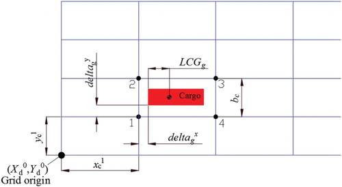
In constraints (2), $|C_{g^{″}}|$ is the number of cells in grid g″ that overlap with grid cell c′, i.e. the constraint is only relevant when these cells overlap (see Figure 1(b)). Before applying these constraints, the grids that are stored in the computer memory are sorted according to the cell size in descending order. Thus, the first grid would be with the largest cell area. Then we check for overlap between larger area cells, c′, with cells of all grids of smaller cell area, c″. This allows notably reducing the amount of constraints controlling the cell overlap. Constraints (3) and (4) make sure that the number of cargo units loaded does not exceed the number of cargo units available for transportation. When all the available cargo units in cargo category g are contractual, i.e. must be loaded, then constraints (3) are used, when the cargo is optional then constraints (4) are activated instead. The number of continuing cargo units has to stay the same across all corresponding loading conditions. To make sure it is the case, constraints (5) are imposed. The constraints are interpreted as the sum of all grid cells in the 1st loading condition must be equal to the sum of these grid cells in any other loading condition. Constraints (6) are activated if continuing cargo must be stowed in the same location throughout the voyage. Constraints (7) control the stowage location of continuing cargo; M is some large number. As discussed in Section 2.3, during the calculation of the shortest path, the shortest path lines on each deck are intersected with other grid cells – belonging to other cargo types – on that deck. As the intersected cells correspond to the binary decision variables, $x_{ldgc}$, these variables are then used for building constraints that eliminate the need of shifting continuing cargo during loading and unloading. Constraints (8) make certain that the total weight of cargo on each deck does not exceed the prescribed maximum carrying capacity of that deck. Constraints (9) control the maximal floor pressure. Thus, grid cells can have different maximal floor pressures and only cargo units that do not exceed the maximal values can be stowed within those cells. The maximal pressure per grid cell is determined from the maximal flood pressure assigned to various areas on the deck (see Figure 2). And when a grid is being created, the cells are being assigned the corresponding maximal values. Constraints (10) are necessary to ensure the stowed cargo height does not exceed the deck ceiling height. As we also consider hoistable panels (or decks), cargo can be stowed either on a panel or under a panel. In both cases, the deck ceiling height is variable. For grid cells being on a panel, the constraints (11) are used. For grid cells under one panel or several panels, constraints (12) are applied.

As explained in (Øvstebø et al. 2011), ship stability calculations involve nonlinear equations. Consequently, the corresponding constraints are also nonlinear, making the MILP model intractable. Therefore, the following constraints have been linearised in a similar fashion as in (Øvstebø et al. 2011; Wathne 2012). Stability constraints on maximal transverse and longitudinal moments are given in (13) and (14), correspondingly. When cargo units are loaded on decks, they create turning moments (torques) with respect to the longitudinal centre line (Y = 0) and transverse centre axis (X = LCG). The resulting roll, $M_r$, and trim,$M_t$, moments are calculated according to (18) and (19), with Figure 7 explaining the meaning of the used parameters. (18) $M_r=\sum _d^{|D|}\sum _g^{|G_d|}\sum _c^{|C_g|}{\text{W}}_g{x}_{dgc}\left(y_c^1+\frac{b_c}{2}+{\delta }_g^y-Y_d^c+Y_d^0\right)$(18) (19) $M_t=\sum _d^{|D|}\sum _g^{|G_d|}\sum _c^{|C_g|}{\text{W}}_g{x}_{dgc}\left(x_c^1+LC{G}_g+{\delta }_g^x-X_d^c+Y_d^0\right)$(19) Given limiting values, $M_r^{max}$ and $M_t^{max}$, are determined based on ballast tank capacity of the vessel (i.e. the capacity to equilibrate the vessel) as described in (Wathne 2012). The capacity can be estimated from general arrangement drawings. Essentially, these constraints make sure that the available capacity of heeling tanks is sufficient to equilibrate the ship.

Stability constraints on acceptable range for metacentric height are aimed to control the transverse metacentric height, GM. It has to be above some minimal value to maintain stability, but also not exceed the assumed maximum to maintain passenger comfort and cargo safety. This is achieved by estimating a new position of the loaded vessel’s VCG, and imposing constraints on its minimal and maximal values. The new vertical position (denoted as Z for short) is calculated as follows: (20) $Z=\frac{{\sum }_d^{|D|}{\sum }_g^{|G_d|}{\sum }_c^{|C_g|}\left(H_d+VC{G}_g\right)W_g{x}_{dgc}+LWT\cdot VCG}{{\sum }_d^{|D|}{\sum }_g^{|G_d|}{\sum }_c^{|C_g|}{W}_g{x}_{dgc}+LWT}$(20) where (21) $\text{VCG = VC}{\text{G}}_0+\frac{{\sum }_p^{|P|}{H}_p{A}_p{w}_p}{LWT}$(21)

As the resulting VCG is constrained to its min and max values, $Z\in \left[Z_{min},Z_{max}\right]$, the corresponding linear constraints (15) and (16) (VCG is not expanded for conciseness). The limiting values, $Z_{min}$ and$Z_{max}$, are determined as described in (Øvstebø et al. 2011). That is, we first recall basic relationships in naval architecture (Derrett and Barras 2006). Then according to DNVGL class rules, the intact GM has to be above 0.15 m (DNV 2012). These values allow calculating$Z_{max}$ as: (22) $Z_{max}=KB\left(T_{max}\right)+BM\left(T_{max}\right)-0.15$(22)

Further, we assume that the natural roll period should not be shorter than some acceptable value, say $T_r\ge 12$ seconds. This allows calculating $Z_{min}$ as follows: (23) $Z_{min}=KB\left(T_{max}\right)+BM\left(T_{max}\right)-\frac{4{\pi }^2{I}_x}{T_r^2\mathrm{\Delta }}$(23)

The use of the above formulae is a linearised method of controlling the GM and the linearisation of constraints is required for linear programming solvers. The use of more accurate, nonlinear relationships can be time prohibitive for practical applications of the stowage optimisation software (Øvstebø et al. 2011).

Constraints (17) are only explicit fire safety constraints on the average headroom on decks. Other the constraints requiring reefers, and other high-risk cargo, to be stowed within designated areas (towards ship stern and along the sides) are implicit. That is, once the designated areas are indicated as input to the programme, only grid cells belonging to high-risk cargo are pre-processed to remove cells being outside the designated areas, as shown in Figure 2. The mandatory longitudinal spacing (Figure 4) is imposed by transversely splitting the deck into subdecks offset by the required spacing. Hence, this constraint is also implicit.

3.6. Solution method

The Ro-Ro ship stowage problem is an NP-hard (Øvstebø et al. 2011) and the computational complexity of a MIP problem depends on the quality of linear relaxation (i.e. bounds), the size of the problem and other factors, and is linear in the number of binary variables, d, provided Brach&Bound algorithm is used (Floudas and Pardalos 2001; Till et al. 2003). An exact relation between d and average complexity of practical problems is unknown but it varies between O(d) to O(2^d) (Zhang 1999). In this paper, the MILP problem was implemented in C++ and solved exactly by the commercial solver by GUROBI³ version 7.02 with default settings. The solver implements the Brach&Bound algorithm.

The numerical example and following calculations in this paper were performed on a laptop running on Windows 7 (64-bit) and powered by Intel(R) Core(TM) i5-6300U CPU @ 2.40 GHz, 8GB RAM.

4. Numerical example

4.1. Assumptions

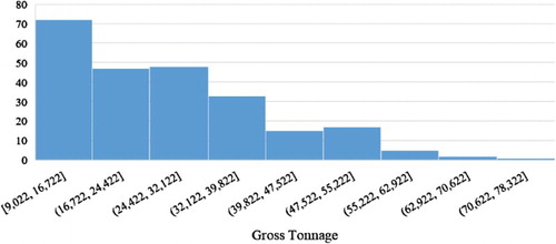
We selected an existing handy size passenger Ro-Ro ship of 14,700 GT (Figure 8); further details can be found in (Zagkas and Pratikakis 2012). The ship of this size was selected on the basis of the GT distribution for passenger Ro-Ro ships worldwide. As Figure 9, the selected ship size falls within the most frequently range used. The data were obtained from the IMO GISIS database by using the search criteria for ship type ‘Passenger/Ro-Ro Ship (Vehicles) (Passenger/Ro-Ro Cargo)’, year of build ‘in or after 2000’, and gross tonnage ‘is more than or equals 9000’. Smaller ship sizes were discarded, for they are typically of the single vehicle deck.

Figure 8. Selected Ro-Ro ship along with relevant parameters.

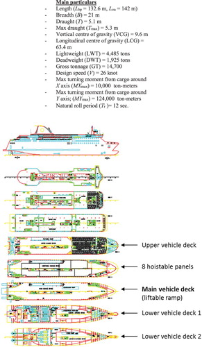
Figure 9. Histogram of worldwide GT distribution for passenger Ro-Ro ships (source: IMO GISIS).

The ship has four fixed Ro-Ro decks and eight hoistable panels (Deck 4) above the main deck (Deck 3), as listed in Table 2. The ceiling height of the main deck is 6 m, and hence the panels are only used above low vehicles such as private cars, vans, and alike. The cargo is loaded and unloaded through the stern ramp on the main deck, and the ramps to lower and upper decks are located towards the starboard. The ramp to Deck 5 can be lifted, allowing stowing cargo underneath on the main deck. The hoistable panels are referred by numbers from 1 to 8, starting from the starboard stern (top left on Figure 8) and going towards the bow, then down towards the port side and the stern (bottom left is panel 8). The panels are independent and only used above lower vehicles (cars, vans, bikes, etc.).

Table 2. Deck dimensions and capacity.

Reference	Breadth (m)	Length (m)	Height (m)	Capacity (tons/m^2)	Weight (tons/m^2)
Main	20	113.3	7.5	10
LLH1	12	43.2	4.5	10
LLH2	12	43.2	1.5	10
Upper deck	20.38	64	11.5	10
Panel1	6.23	22.06	7.5–11.5	3	0.1
Panel2	6.23	24.15	7.5–11.5	3	0.1
Panel3	9.93	14.4	7.5–11.5	3	0.1
Panel4	9.93	20.61	7.5–11.5	3	0.1
Panel5	9.31	20.61	7.5–11.5	3	0.1
Panel6	9.31	19.2	7.5–11.5	3	0.1
Panel7	6.93	24.15	7.5–11.5	3	0.1
Panel8	9.26	22.06	7.5–11.5	3	0.1

Each deck has a set of attributes such as dimensions and areas to be excluded (Figure 2), maximal payload and capacity (floor pressure), and others (Table 2). Together with the cargo attributes, these attributes are used to generate cargo type-related grids for each deck. The attributes of typical cargo categories are listed in Table 3 (Wathne 2012). This table was used to generate a pool of cargo to be loaded in each port of call. The presence of a specific cargo category in a given port was determined with turn-up probability that changes from port to port. Figure 10(a) shows a sample distribution for cargo turn-up probability, whereas the actual number of cargos is also randomly selected from the uniform range [0, n_max] with n_max values shown in Figure 10(b). Both distributions are hypothetical and reflect a route that is dominated by low vehicles (private cars, vans).

Figure 10. Sample cargo turn-up probability (a) and the maximal number of cargo per turn-up (b).

Table 3. Sample Ro-Ro cargo categories (only main attributes are shown).⁵

Cargo category	Breadth (m)	Length (m)	CEU^6	Height (m)	Weight (MT)	LCG (m)	VCG (m)	Revenue per trip
Motobike (Ducati)	0.78	2.00	0.24	1.08	0.21	1.00	0.16	50
Toyota	2.00	4.85	1.52	2.00	1.35	2.43	0.54	290
Toyota (electric)	2.00	4.85	1.52	2.00	1.35	2.43	0.54	290
VAN (Boxer)	2.51	4.96	1.94	2.25	3.00	1.49	0.79	290
Semi-trailer	2.80	13.57	5.94	4.50	15.00	6.79	2.47	388
Container (FEU, type 1 AA)	2.80	12.40	5.43	3.95	23.00	6.20	1.38	400
Supermini (Opel Corsa, VW Polo)	1.68	3.98	1.05	1.45	1.06	1.19	0.51	150

This way, we randomly create a sample itinerary with cargo distributions in each port, assuming the maximal number of cargo categories in port to be five. Table 4 lists generated cargo load across three ports. The majority of cargo is optional (=1), which means it is only transported if space is left on the deck after all contracted cargo have been loaded. In other practical cases, the contracted cargo might represent the majority.

Table 4. Randomly generated cargo distribution in three ports of call (two loading conditions).

#	Category	Reference (port in | port out-CEU)	Number in category	Optional	Loading port	Unloading port	Allowed decks
1	VAN	1|3-1.9	150	1	1	3	All
2	Semi-trailer	1|2-5.9	2	0	1	2	Main deck only
3	Toyota	1|2-1.5	180	1	1	2	All
4	Toyota (electric)	1|2-1.5e	180	1	1	2	Main deck only
5	Supermini	1|2-1.0	300	1	1	2	All
6	Container	1|2-5.4	2	0	1	2	Main deck only
7	Toyota	2|3-1.5	150	1	2	3	All
8	Toyota (electric)	2|3-1.5e	34	1	2	3	Main deck only
9	VAN (Boxer)	2|3-1.9	150	1	2	3	All
10	Semi-trailer	2|3-5.9	2	0	2	3	Main deck only
11	Container	2|3-5.4	2	0	2	3	Main deck only
12	Supermini	2|3-1.0	150	1	2	3	All

4.2. Result 1

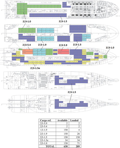
This subsection displays the results when the fire safety constraints were deactivated. Displayed stowage plans are followed by a result table showing the cargo distribution per deck, deck area utilisation and deck’s elevation above the main deck, if the deck is hoistable. For better readability of Figure 11 and Figure 12, cargo references are given. One can notice that the third hoistable deck (port side) on Figure 11 is not used, due to high cargo (1|2-5.9) underneath and no small enough cargo available to load it.

Figure 11. Optimal stowage plan for the 1st loading condition (Port 1 – Port 2).

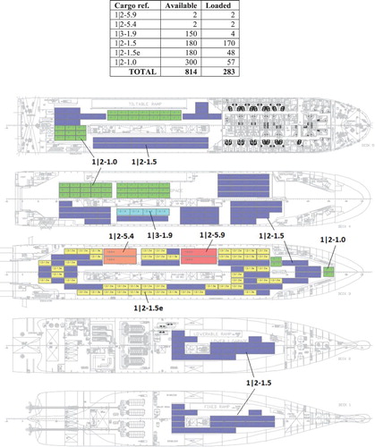
Figure 12. Optimal stowage plan for the 2nd loading condition (Port 2 – Port 3).

4.3. Result 2

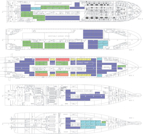
This subsection shows the results obtained after the introduction of the fire constraints, while using the same cargo load shown in Table 4. The activated fire constraints ensured the longitudinal clearance between vehicles (clearance of 60 cm every 20 m), high-risk cargo (reefers and electric cars) to be stowed on the designated area on the main deck, and the average headroom to be above the required one. Figure 13 shows the illustrative designated areas for reefers and electric cars, whereas the optimal stowage plans for both loading conditions are shown in Figure 14 and Figure 15. Note, the first three hoistable decks (port side) on Figure 14 are not used (empty) due to high cargo underneath and available low cargo that would still fit on the hoistable decks stowed in other locations.

Figure 13. Assumed designated areas for reefers and electric cars: the areas are on the main deck only and along both ship’s sides.

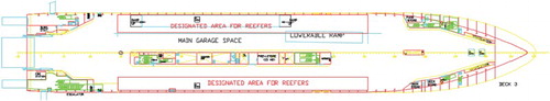
Figure 14. Optimal stowage plan for the 1st loading condition (Port 1 – Port 2) with active fire constraints on the main deck.

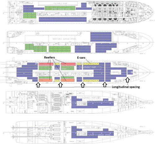
Figure 15. Optimal stowage plan for the 2nd loading condition (Port 2 – Port 3) with active fire safety constraints on the main deck.

5. Sensitivity analysis

5.1. Effect of fire safety constraints on revenue

This section demonstrates the effect of the introduced fire safety constraints on the net revenue (Section 2.2 and Equation (17)). This was achieved through sensitivity analysis by randomly varying the cargo distribution and parameters for a fixed itinerary and ship configuration presented in Section 4. As the constraints can be treated as fire risk control measures, the results can be helpful in the future analysis of their cost-effectiveness. The analysis itself is outside the scope of this paper, as it also requires estimating the effect on fire risk.

The following fire constraints were introduced one at a time, calculating the effect on the net revenue:

1. Constraints on the average headroom to improve the effectiveness of the drencher system.

2. Constraints introducing the longitudinal spacing by transversely splitting the main deck into subdecks.

3. Constraints requiring reefers, and other high-risk cargo such as electric cars, to be stowed within designated areas (typically towards ship stern and along the sides).

4. All constraint types are active.

Figure 16 shows the boxplots of the relative reductions in the net revenue (maximised during the optimisation). The reductions are shown with respect to a reference case where the fire safety constraints were not applied. Each boxplot was obtained based on 20 sample points.

Figure 16. Boxplots of individual and combined reduction from fire safety constraints in the total net revenue per voyage.

As the result shows, the spacing constraints have the biggest negative potential on the revenue. This is self-explanatory, because they explicitly remove a significant share of useful cargo space. The combined effect of the constraints may lead to some 20% reduction in the net revenue. It should be noted, however, that these estimates are conditional on the assumed ticket prices (Table 3), distributions of cargo types and their numbers (Figure 10).

5.2. Effect on computation time

The intention of this section is more practical than academic. We investigate the link between problem characteristic parameters and computational cost (CPU time). In this analysis, we assume that the ship configuration, i.e. the number and capacity of decks, is fixed and only the payload configuration (the numbers and types of vehicles) varies.

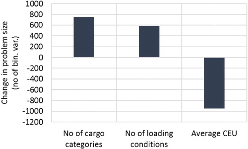
The problem size is driven by the number of binary variables and constraints, which in turns is driven by characteristic parameters such as the number of cargo categories (i.e. the number of grids per deck), the number of decks, and the floor area of cargo units, i.e. the number of cells in grids (grid fineness). The number of available cargo units within a cargo category was found to have an insignificant effect on the CPU time and it was ignored. Thus, three independent, characteristic parameters that control the problem size are:

• Number of cargo categories

• Average of CEU across cargo categories

• Number of loading conditions (proportional to the number of ports of call)

We assumed the following uniform distributions for these parameters, [2,15], [1,5], and (0.24, 3.3), and generated 300 random samples of payload configurations (cargo distributions). Figure 17 shows the distribution of calculated CPU time across these samples. Thus, 50% of cases would finish within some 20 min, whereas 75% cases would be completed within an hour.

Figure 17. Boxplot for computational cost (CPU time in minutes).

Assuming that the problem size, and hence CPU time, is proportional to the number of binary variables, the runs were used to regress a linear model of which partial regression coefficients shown in Figure 18. Evidently, the average CEU has the biggest effect on the number of binary variables as a fall in CEU leads to finer grids and hence more alternative stowage locations (∼1000 more binary variable when average CEU is decreased by 1).

Figure 18. Partial regression coefficients (main effects)⁴ showing the change in the number of binary variables (on average) corresponding to a unit change in the displayed input parameters.

6. Conclusions

The paper has dealt with the optimal cargo stowage problem on Ro-Ro decks, which stow heterogeneous cargo along a multi-port journey. In view of the existing attempts to solve this stowage problem, the paper has proposed the three practical improvements with respect to the state of the art. As a result, a solution to the stowage problem leads to a better treatment of ship stability, fire safety, and cargo handling efficiency. The proposed improvements are summarised as follows:

• The proposed discretisation of deck areas removes the uncertainty about the cargo location and enables precise ship’s stability and other calculations. It also introduces complete certainty about the grid resolution, as the grid cells always reflect the corresponding cargo size.

• New constraints for fire safety on Ro-Ro decks have been developed and their effect on the optimisation results has been examined. The results can serve as a basis for future analysis of cost effectiveness of the proposed fire risk control measures.

• Stowage plans that ensure zero shifting cost during loading/unloading.

There are a few caveats to our approach we would like to highlight. We have solely focused on formulating the MILP problem, leaving the challenge of solving it to available solvers. The mathematical formulation ends up with tens of thousands of variables and constraints for a medium size Ro-Ro ship, with the problem size being largely driven by the cargo dimensions. However, the case studies show that the problem is solvable by commercial MILP solvers in a reasonable time (Section 5.2). The proposed formulation does not explicitly group cargo of the same type. However, the cargo can be assigned to designated areas where it would become adjacent. The effect of passengers on ship stability was ignored, assuming it is negligible compared to the cargo load. We also recognise that the optimal stowage problem should ideally be solved as part of tactical and strategical decisions (Christiansen et al. 2007). However, the benefits can be demonstrated already now, whereas the holistic solution – being potentially more beneficial – seems intractable at present.

Acknowledgements

This presented work used IT and other resources of the Maritime Safety Research Centre of University of Strathclyde, which is kindly acknowledged for providing them.

Disclosure statement

No potential conflict of interest was reported by the author.

ORCID

Romanas Puisa http://orcid.org/0000-0002-4487-6392

Notes

1 A vehicle that runs on a fuel other than traditional petroleum fuels (petrol or diesel fuel), such as electric cars, hybrid electric vehicles, hydrogen, LNG and LPG.

2 Unless stated otherwise, the constraints are written – for the sake of simplicity – within a single cargo-loading condition, consequently omitting subscript l.

3 http://www.gurobi.com

4 Multiple regression model, (R²> 0.9), was developed with main effects only and no intercept.

5 Cargo attributes were found on public websites, as well the ticket prices, which were found on ferry booking portals.

6 The car equivalent unit (CEU) is based on the dimensions of a 1966 Toyota Corolla model RT43, which is 13.5 feet (4.125 m) × 5 feet (1.55 m) × 4.6 feet (1.4 m). The ground space required for a CEU RT43 is approximately 69 sq. ft. (6.4 sq. m) and the ground slot, including spacing in between vehicles is 80 sq. ft. (7.4 sq. m).

References

- Avriel M, Penn M. 1993. Exact and approximate solutions of the container ship stowage problem. Comput Ind Eng. 25(1–4):271–274. doi: 10.1016/0360-8352(93)90273-Z
- Christiansen M, Fagerholt K, Nygreen B, Ronen D. 2007. Maritime transportation. Handbooks in Operations Research and Management Science. 14:189–284. doi: 10.1016/S0927-0507(06)14004-9
- Derrett D, Barras C. 2006. Ship stability for masters and mates. Heinemann: Elsevier Butterworth.
- Ding D, Chou MC. 2015. Stowage planning for container ships: a heuristic algorithm to reduce the number of shifts. Eur J Oper Res. 246(1):242–249. doi: 10.1016/j.ejor.2015.03.044
- DNV. 2012. Hull equipment and safety. In: Rules for classification of ships. Oslo, Norway: DNV; p. 125–126.
- Floudas CA, Pardalos PM. 2001. Encyclopedia of optimization. Alphen aan den Rijn, Netherlands: Kluwer Academic Publishers.
- Hansen JR, Hukkelberg I, Fagerholt K, Stålhane M, Rakke JG. 2016. 2D-Packing with an Application to Stowage in Roll-On Roll-Off Liner Shipping. 7th International Conference, ICCL 2016, Lisbon, Portugal, September 7–9; Springer; 2016. p. 35–49.
- Hart PE, Nilsson NJ, Raphael B. 1968. A formal basis for the heuristic determination of minimum cost paths. IEEE Transactions on Systems Science and Cybernetics. 4(2):100–107. doi: 10.1109/TSSC.1968.300136
- Jansson JO, Shneerson D. 1987. Liner shipping economics. London: Chapman and Hall Ltd.
- Mulder J, Dekker R. 2016. Optimization in container liner shipping (No. EI2016-05). Econometric Institute Research Papers. http://hdl.handle.net/1765/79911.
- Øvstebø BO, Hvattum LM, Fagerholt K. 2011a. Optimization of stowage plans for RoRo ships. Comput Oper Res. 38(10):1425–1434. doi: 10.1016/j.cor.2011.01.004
- Øvstebø BO, Hvattum LM, Fagerholt K. 2011b. Routing and scheduling of RoRo ships with stowage constraints. Transp Res C, Emerg Technol. 19(6):1225–1242. doi: 10.1016/j.trc.2011.02.001
- Pacino D, Delgado A, Jensen R, Bebbington T. 2011. Fast generation of near-optimal plans for eco-efficient stowage of large container vessels. In: Böse JW, Hu H, Jahn C, Shi X, Stahlbock R, Voß S, editors. Computational logistics. ICCL 2011. Lecture notes in computer science, Vol 6971. Berlin, Heidelberg: Springer.
- Pacino D, Delgado A, Jensen RM, Bebbington T. 2012. An accurate model for seaworthy container vessel stowage planning with ballast tanks. ICCL: Springer. p. 17-32.
- Parreño F, Pacino D, Alvarez-Valdes R. 2016. A GRASP algorithm for the container stowage slot planning problem. Transport Res E Log. 94:141–157. doi: 10.1016/j.tre.2016.07.011
- Seixas MP, Mendes AB, Barretto MRP, Da Cunha CB, Brinati MA, Cruz RE, et al. 2016. A heuristic approach to stowing general cargo into platform supply vessels. J Oper Res Soc. 67(1):148–158. doi: 10.1057/jors.2015.62
- Siewers HE, Tosseviken A. 2016. Fires on Ro-Ro decks. Oslo, Norway: DNV GL.
- Tang L, Liu J, Yang F, Li F, Li K. 2015. Modeling and solution for the ship stowage planning problem of coils in the steel industry. Naval Research Logistics (NRL). 62(7):564–581. doi: 10.1002/nav.21664
- Till J, Engell S, Panek S, Stursberg O. 2003. Empirical complexity analysis of a MILP-approach for optimization of hybrid systems. IFAC Conference on Analysis and Design of Hybrid Systems 2003. p. 129-34.
- Ware K. 2017. State of the industry regulatory developments. passenger ship safety conference. Southampton: TDN UK.
- Wathne E. 2012. Cargo stowage planning in RoRo shipping: optimisation based naval architecture. Trondheim, Norway: Institutt for Marin Teknikk.
- Wikman J. 2016. Study investigating cost effective measures for reducing the risk from fires on ro-ro passenger ships (FIRESAFE). Lisbon, Portugal: EMSA.
- Wilson I, Roach P. 2000. Container stowage planning: a methodology for generating computerised solutions. J Oper Res Soc. 51(11):1248–1255. doi: 10.1057/palgrave.jors.2601022
- Wilson ID, Roach PA. 1999. Principles of combinatorial optimization applied to container-ship stowage planning. J Heuristics. 5(4):403–418. doi: 10.1023/A:1009680305670
- Zagkas V, Pratikakis G. 2012. Specifications of cargo and passenger ships. EC FP7 project FAROS (no 314817): Naval Architecture Progress; 2012.
- Zhang W. 1999. State-space search: algorithms, complexity, extensions, and applications. New York: Springer-Verlag.