Modelling and performance prediction of a centrifugal cargo pump on a chemical tanker

Abstract

In this paper, a single-stage, horizontal type centrifugal pump, which can be used in a chemical tanker’s cargo operations, was modelled with MATLAB/Simulink software. The modelled pump was run with seven different fluids handled in chemical tankers which are ethyl alcohol, N-Propyl alcohol, phenol, chloroform, castor oil, 55% nitric acid and water. Therefore, the pump’s performance curves and data sets were obtained for each situation. After these, a neural network was created with MATLAB/ Neural Network Fitting Tool application. Inputs of the network were volumetric flow, head, shaft power, torque, and net positive suction head. The output was the pump efficiency and it is estimated for each fluid from the numeric data. Mean squared error was very close to zero (1.1817e-6) and R² provided a prediction accuracy of 99.996%. According to these results, artificial neural network (ANN) had a satisfactory performance to predict the efficiency of a chemical tanker’s centrifugal cargo pump.

1. Introduction

The installation cost of a pumping system is 8% of total costs; however, their operating expenses are 60% of the overall running expenditures (Yumurtaci and Sarıgul 2011). According to Ertoz (2003) pumps use 20% of consumed energy that brings them on the first rank. Moreover, design improvements and proper pump selection according to the operating conditions can save 30% of the energy (Kaya et al. 2008). In ships, many auxiliary systems have pumping equipment, and their energy consumption is remarkably higher compared with other equipment. They disburse approximately 50% of the electrical power produced at the ship (Durmusoglu et al. 2015; Kocak and Durmusoglu 2017).

Centrifugal pumps are commonly used both inshore facilities and onboard. They are widely used for the water transfer on board. Moreover, in a liquid bulk carrier, they can be used as the cargo transfer pump which is desired for handling various liquids (Sakar and Zorba 2013). For this reason, the efficiency of centrifugal pumps has become increasingly important for marine engineers. That is why, predicting, optimising and increasing the pump efficiency are crucial subjects for decreasing the cost and improving to system performance.

Chemical tankers are expected to spend less hours in a port that’s why, increased transfer speeds are required and demanded by port authorities and ship owners. Besides, during a cargo discharge operation, safety of the environment and the crew is a crucial issue to consider. Therefore, reliable cargo transfer pumps have a significant role to achieve these demands (Sakar and Zorba 2013). Modelling and using ANN for prediction of the chemical tanker cargo pumps’ performance is a novel and an applicable approach for an operating pump. Cargo transfer operations for a chemical tanker can be optimised with using these methods. They can be helpful for condition monitoring of the cargo pump so the efficiency losses can be detected.

Some research streams focused on achieving these goals. These studies used both the design and the operating parameters of the centrifugal pumps to improve or to estimate the efficiency by using various algorithms and techniques. Benini and Cenzon (2009) conducted a study about calibrating centrifugal pumps, using an evolutionary algorithm and achieved to increase the efficiency of the system. Sakthivel et al. (2010) employed methods such as fuzzy logic, neural networks and decision tree to estimate faults of a pump using the vibration data. Azadeh et al. (2010), also conducted a study on the maintenance process of pumps by using fuzzy logic. Nourbakhsh et al. (2011) applied a design optimisation for a centrifugal pump with colony optimisation and artificial neural networks (ANNs). Sakthivel et al. (2012), performed another study about vibration signals based on fault diagnosis and estimation using fuzzy logic, neural networks and decision trees. Azadeh et al. (2013) compared neural networks, genetic algorithm and colony optimisation according to their performance estimation successes. Derakhshan et al. (2013), focused on the impeller geometry optimisation by applying neural networks and colony optimisation algorithm methods. Wu et al. (2014) conducted a genetic algorithm to increase energy efficiency of the parallel pumping system. Su et al. (2015) used the colony optimisation for fault diagnosis on rotating machinery. An et al. (2016) employed the evolutionary algorithm for multi-objective optimisation of low-speed centrifugal pumps. They also performed a numerical simulation based on Reynolds averaged Navier-Stokes turbulent model. The results showed that unexpected flows were not shown in the optimised pump. Olszewski (2016) examined load optimisation on a system which has four centrifugal pumps by using genetic algorithm. Wang et al. (2017) published an article about impeller analysis for improving the efficiency and comparison of techniques for performance prediction. Lomakin et al. (2017), studied about flow optimisation of pumps. Moreover, some recent studies have employed ANNs in marine engineering. Nowruzi et al. (2017) used computational fluid dynamics and ANNs to predict the performance of submerged hydrofoils. Shora et al. (2018), applied computational fluid dynamics and ANN to predict the performance and cavitation volume of a propeller under different geometrical physical characteristics. Taghva et al. (2018), applied ANN to estimate the seakeeping performance under irregular wave conditions in a container ship. Najafi et al. (2018), used neural networks and experiments to predict the performance of hydrofoil-supported catamarans. Derakhshan and Bashiri (2018), assessed the shape optimisation with ANN and Eagle Strategy algorithms on centrifugal pumps. The optimised geometry improved the efficiency and head of the pump.

As a result of the literature review on optimisation of the centrifugal pumps, the main theme of the studies could be categorised as design optimisation of the volute, the diffuser and impeller blades, load optimisation of parallel pumps, the performance or fault diagnosis and estimation. It is observed that the studies predominantly focus on centrifugal pumps in shore facilities. In light of the literature review, there are no studies on centrifugal pump performance estimation while handling different chemicals. Thus, this study aims to fill this gap in the literature. Performing artificial intelligence for a ship for operational level is a novel approach and which can be helpful for condition monitoring and performance evaluation of the equipment in the ship engine room.

In this study, the efficiency prediction of a centrifugal pump was performed by using the ANN. The selected pump can be used for loading/unloading operations in chemical tankers. Modelling and using ANN for prediction of the chemical tanker cargo pumps’ performance is a novel approach for an operating pump. This is a helpful step for condition monitoring of the cargo pump so the efficiency losses can be detected and fixed. Transfer delays can be lowered using these analyses properly. As the first step of the study, a horizontal type single stage centrifugal pump was modelled with its total head (H) – volumetric flow rate (Q), pump efficiency(η)-Q, shaft power(P)-Q, required net positive suction head (NPSH_r)-Q graphs, using MATLAB/Simulink software. Then, the modelled pump was run with seven different liquids such as, water, ethyl alcohol, N-Propyl alcohol, phenol, chloroform, castor oil and 55% nitric acid. Thus, performance curves and data sets for each condition were obtained numerically. An ANN was created with MATLAB/Neural Network Fitting Tool application and the network was trained with these data sets. In this study, the efficiencies for each condition were estimated with acceptable error rates in the result of some trials.

2. Methodology

Simulink application of MATLAB is used for modelling the centrifugal pump.

Simulink® is a block diagram environment for multidomain simulation and Model-Based Design. It supports simulation, automatic code generation, and continuous test and verification of embedded systems. Simulink provides a graphical editor, customizable block libraries, and solvers for modeling dynamic systems

(Mathworks 2018). Performance diagrams, operational information, pipe lengths and design parameters were provided by Gemlik Fertilizer Industry Inc.

Total head (H), specific speeds (n_q), torque, pump efficiency and NPSHr equations were coded to the model with using taken data. The pump efficiency can be calculated by Equation (1). (1) $\eta =\frac{\rho gHQ}{1000P}$(1) The total head can be described as the pump’s ability to raise the liquid to a specific height or ability to develop a given discharge pressure. It can be found with the sum of the static head (H_s), pressure head (H_p), velocity head (H_v) and losses head (H_L). These components can be obtained with the following equations (Bachus and Custodio 2003): (2) $\begin{array}{rl}H& =H_{\text{s}}+H_{\text{p}}+H_{\text{v}}+H_{\text{L}}\end{array}$(2) (3) $\begin{array}{rl}{H}_{\text{s}}& =z_{\text{d}}-z_{\text{s}}\end{array}$(3) (4) $\begin{array}{rl}\text{Hp}& =(p_{\text{d}}-p_{\text{s}})/\rho g\end{array}$(4) (5) $\begin{array}{rl}{H}_{\text{v}}& =(v_{\text{d}}^2-v_{\text{s}}^2)/2g\end{array}$(5) (6) $\begin{array}{rl}{H}_{\text{L}}& =h_{\text{f}}-h_{\text{m}}\end{array}$(6)

Equation (7) illustrates the NPSH_r formula. (7) $NPS{H}_{\text{r}}=P_{\text{atm}}+P_{\text{g}}+H_{\text{v}}-H_{\text{vp}}$(7) In these equations, P_atm represents the atmospheric pressure, and P_g stands for the gauge pressure. The height of discharge line is z_d and z_s is height of suction side. Discharge pressure is p_d, and the suction pressure is p_s. Fluid velocity at discharge side is v_d and velocity at suction side equals to v_s. In order to determine H_L, pipe losses (h_f) and valve-fitting and elbow losses (h_m) are to be found. For pipe losses, Darcy-Weisbach formula was used because it provides the most accurate results for various applications (Bachus and Custodio 2003). Friction coefficient (f) is calculated with Colebrook equation, and relative roughness was obtained from tables according to pipe material. Losses of valves, fittings and elbows were calculated from tables, and their angles, materials and number of the connection elements in the circuit were specified at the factory and from piping diagrams.

Selected pump handles different liquids, and these fluids are also handled in chemical tankers. In the model, flow rate was increased linearly from 0 to 30 by adding 0.1 m³/h in each step. Power was also increased linearly from 5.5 to 9, and its increment depends on the flow rate. Pump capacity and size is also compatible with chemical tanker cargo pump. After the Simulink model was formed, seven different liquids were selected according to their densities and viscosities. Water is the reference fluid for the pump model. Chemicals with various viscosities and densities were tried in the model to observe density and viscosity effects of the fluid on the pump performance. Table 1 illustrates the properties of the chemicals chosen from IBC Code. Viscosity and density values were obtained by accepting fluids at 20°C. After that, the pump model was run with these liquids thus, flow rate versus power, head, required net positive suction head, efficiency and torque graphs were obtained. Besides, the data sets obtained numerically from the model were scaled and prepared for the ANN application. Simulink model of the pump is shown in Figure 1.

Figure 1. Simulink model of the centrifugal pump.

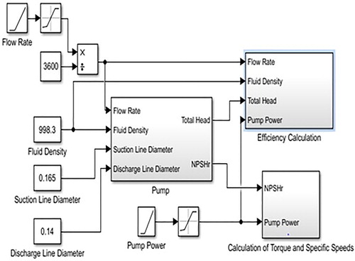
Table 1. Properties of chemicals used in the model (IMO 2016; Pillon 2007).

Index Name	Product Name	Density (kg/m^3)	Kinematic Viscosity (cst)	Hvp (Pa)
Ethanol	Ethyl Alcohol	772	1.51	9000
Propanol	N-Propyl Alcohol	804	2.8	2400
Benzenol	Phenol	1078	11.3	500
Trichloromethane	Chloroform	1489	0.38	30,000
Ricinus Oil	Castor Oil	960	1017	0
Water	Water	997	1.003	2330
Nitric Acid (Less than 70%)	Nitric Acid(Less than 70%)	1339	5	7700

ANN, which are one of the artificial intelligence algorithms, have a wide use area in line with these purposes. The network can be trained and it can improve or estimate the future conditions with using various data (Dreyfus 2005). In order to achieve a successful performance estimation, MATLAB Neural Network Fitting Tool is used to create an ANN. The crucial components of ANN are number of layers and neurons. In order to discover an adequate number of layers, neurons and the training-test split ratio, various trials are to be carried out (Oztemel 2016; Köseoğlu 2015). Table 2 illustrates the trials and the other network information.

Table 2. ANN model specifications.

Neural network type	Feed-forward backpropagation
Training function	Levenberg-Marqurdt
Learning function	Gradient descent with momentum weight and bias learning function (Learngdm)
Performance measurement function	MSE
	R-squared
Number of layers	1–5
Number of neurons	1–20
Training-validation-test split percentage	90%–5%–5%
	80%–10%–10%
	70%–15%–15%
	60%–20%–20%
Transfer (Activation) Function	Hyperbolic tangent sigmoid transfer function (Tansig),
	Linear transfer function (Purelin)

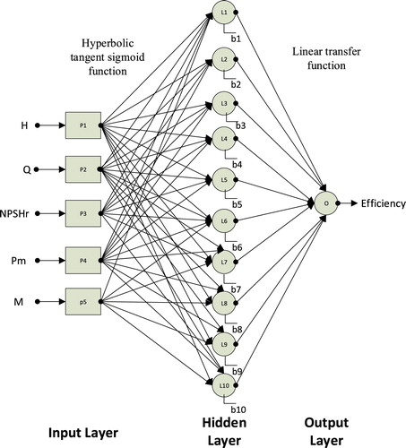
The number of layers was tried from 1 to 5. Using one hidden layer and one output layer provided the optimum results in this model. Besides, the number of neurons were tried from 1 to 20, and it was decided 10 neurons as the result of trials. Levenberg-Marqurdt, Bayesian Regularization, Scaled Conjugate Gradient algorithms were tried as the training function. The model with Levenberg-Marqurdt algorithm had a better performance to optimise the ANN parameters (bias and weights). The algorithm has wider usage in similar studies. Training, validation and testing percentages of the network were determined by experiencing different variations to avoid the overfitting. After the trials, 70% training, 15% validation and 15% testing were decided. Inputs of the network are Q, H, NPSH_r, Pm and M. The parameters were selected with the aid of the model’s mathematical relations and examining of similar studies. The output is the efficiency thus, the network can estimate the model performance. Min–max normalisation of data was applied before using in the network. The following equation was used for normalisation: (8) ${\mathrm{\varnothing }}_n=0.8\frac{\mathrm{\varnothing }-min(\mathrm{\varnothing })}{max(\mathrm{\varnothing })-min(\mathrm{\varnothing })}+0.1$(8) where ${\mathrm{\varnothing }}_n$ is the input value after normalisation process (Khataee and Kasiri 2010). The supervised learning was performed with feed-forward back propagation neural network. Thus, the output will be informed by the input layer. Then, the input variables are transferred via these layers. The transfer process was carried out by the transfer function. After that, the variables participate in hidden layers through input and hidden layer neurons’ liaison. Because of the weights of the neurons, the fundamental estimates in the ANN are shrouded. Neurons of the hidden layer weight the sum of the previous layers’ outputs. Then the bias measures the former information and sum of the outputs transfer through the transfer function (Taghva et al. 2018). The hyperbolic tangent sigmoid function was determined as an activation function because it was repeatedly tested and used frequently by the existing studies. The function was defined as follows: (9) $n_j=\frac{2}{1+e^{-2Z}}-1$(9) In this equation, n_j is the neuron’s output, and Z can be calculated as follows: (10) $Z=\sum _{i=1}^r{\omega }_{ij}{p}_i+b_j$(10) ω_ij is the linkage weights of the i_th neuron in the previous layer to the j_th neurons and p_i is the output of the i_th neuron. Number of neurons from the previous layer and the bias are r and b_j, respectively (Najafi et al. 2018). The output layer transfer function is a linear transfer function (λ). (11) $g=\lambda ({\omega }_{L}Z+b_0)$(11) where ${\omega }_L$ is the interconnection weights between the tail ender hidden and output layers. b₀ is the output layer bias (Taghva et al. 2018). Neural Network Fitting Tool uses last two functions as the activation and the output functions. The researchers proposed the performance functions to measure accuracy and to determine error rate of the model. In this study, performance function was determined ‘Mean Squared Error (MSE)’ in the tool. The smaller MSE value means a lower margin of error (Allen 1971). The correlation coefficient (R) and its square was applied to define the strength of the predictions. If the square of the correlation coefficient closes 1, the relationship is stronger (Bluman 2000). MSE and R formulation are illustrated as follows (Armstrong and Collopy 1992; Makridakis et al. 1998): (12) $\begin{array}{rl}MSE& =\frac{\sum _{i=1}^N{(O_i-y_{desired})}^2}{N}\end{array}$(12) (13) $\begin{array}{rl}R& =1-\frac{\sum _i^N(O_i-y_{desired})}{\sum _i^N(O_i-{\overline{y}}_{desired})}\end{array}$(13) where, the number of the input data is N, reference data is $y_{desired}$, predicted outcomes are O_i, and the mean of desired values are ${\overline{y}}_{desired}$ (Najafi et. al 2018). Figure 2 shows the network’s structure. Figure 3 illustrates the architecture of selected ANN for the performance estimation.

Figure 2. Basic structure of the network.

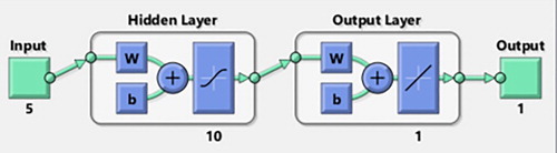
Figure 3. The architecture of selected ANN in the performance estimation.

3. Results and discussion

When the pump operated with the liquids mentioned in Table 1, H, NPSH_r and η at the optimum flow rate (15 m³/h) were obtained from the model. Table 3 illustrates the results.

Table 3. Model outputs at the optimum flow rate.

Product name	H (m)	NPSHr (m)	η
Ethyl alcohol	93.786	1.444	0.423
N-propyl alcohol	89.933	0.895	0.422
Phenol	66.305	2.697	0.423
Chloroform	47.167	6.370	0.409
Castor Oil	74.827	1.907	0.419
Water	70.045	2.701	0. 394
Nitric acid 55%	50.99	5.12	0.380

The head is inversely proportional to the fluid density. It can be seen that the efficiency increases while the density of liquids decreases. The kinematic viscosity and the vapour pressure of the fluid also affect the overall efficiency of the pump. The castor oil is the most viscous fluid among others, and its vapour pressure is 0. Its density is close to the reference liquid (water). As a result of the comparison between these liquids, it was determined that the pump efficiency and head increase when the fluid has higher viscosity and lower vapour pressure. The analogy between Chloroform and nitric acid indicated that the higher vapour pressure leads to the head drop. Furthermore, net positive suction head required was more elevated when the vapour pressure and density of fluid are higher. This leads to the opening of the difference between the net positive suction head acquired and the net positive suction head required, in other words, cavitation. If there is a significant increase in the fluid density relative to the reference value, it is observed that the pump head is significantly reduced.

As a result of working with various fluids, seven different data sets with 301 samples were obtained. These data sets were normalised with min-max normalisation and organised to estimate efficiency for different fluids by neural networks. By using training and working of the network, estimation errors, R-values, R² values, MSE values and efficiency estimations are obtained. Figure 4 indicates the validation performance and regression analysis graphs for the data set of the water. R-value was obtained 0.99998 and R² provided a prediction accuracy of 99.996%. Table 4 shows inputs, output estimations and errors for water. MSE of the model for handling water was very close to 0 (1.1817e-6). The best validation performance was also close to 0 (8.4495e-7) which was reached at epoch 42.

Figure 4. Results of ANN with water’s dataset: Validation performance (a) Regression analysis graphics (b).

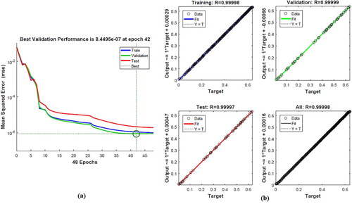
Table 4. ANN data and errors for water.

Q (m^3/h)	H (m)	NPSHr (m)	Pm (kW)	Torque (N.m)	Efficiency	Predicted efficiency	Error
0	69.8673	2.7028	5.5000	17.8942	0.0000	0.008533	−0.00853
2	69.8705	2.7028	5.7330	18.6523	0.0663	0.066339	−3.1e-05
4	69.8800	2.7027	5.9660	19.4103	0.1275	0.127272	0.000183
6	69.8959	2.7026	6.1990	20.1684	0.1840	0.183911	0.000127
8	69.9181	2.7024	6.4320	20.9265	0.2366	0.237066	−0.0005
10	69.9467	2.7022	6.6650	21.6845	0.2855	0.285636	−0.00014
12	69.9816	2.7019	6.8980	22.4426	0.3312	0.330769	0.000415
14	70.0229	2.7016	7.1310	23.2007	0.3740	0.37363	0.000347
16	70.0705	2.7012	7.3640	23.9587	0.4142	0.414418	−0.00026
18	70.1245	2.7008	7.5970	24.7168	0.4520	0.45246	−0.00047
20	70.1848	2.7004	7.8300	25.4748	0.4877	0.52101	0.000436
22	70.2514	2.6998	8.0630	26.2329	0.5214	0.554075	−0.00063
24	70.3245	2.6993	8.2960	26.9910	0.5534	0.583232	0.000615
26	70.4038	2.6987	8.5290	27.7490	0.5838	0.61401	−0.00123
28	70.4895	2.6980	8.7620	28.5071	0.6128	0.635046	0.005336
30	70.5816	2.6973	8.9950	29.2652	0.6404	0.008533	−0.00853

When the ANN model was constructed with ethyl alcohol, MSE was very close to 0 (8.35e-5). Figure 5 indicates validation performance and regression analysis graphs of ANN. Table 5 illustrates inputs, the output, ANN estimations and errors. The best validation was obtained at epoch 127 and its performance was close to zero (0.00014746). R was obtained as 0.9988 and R² provided a prediction accuracy of 99.76% which was in an acceptable range of accuracy.

Figure 5. Results of ANN with ethyl alcohol’s data set: Validation performance (a) Regression analysis graphics (b).

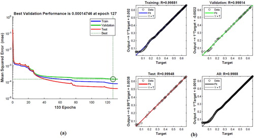
Table 5. ANN data and errors for ethyl alcohol.

Q (m^3/h)	H (m)	NPSHr (m)	Pm (kW)	Torque (N.m)	Efficiency	Predicted efficiency	Error
0	93.61356	1.444169	5.5000	16.26746	0.003939	0.054827	−0.05089
2	93.61663	1.444169	5.7330	17.09444	0.074966	0.061647	0.013319
4	93.62586	1.444169	5.9660	17.96494	0.14268	0.128787	0.013894
6	93.64125	1.444169	6.1990	18.83544	0.204163	0.216045	−0.01188
8	93.66279	1.444169	6.4320	19.70594	0.260252	0.2568	0.003451
10	93.69049	1.444169	6.6650	20.57643	0.311644	0.31445	−0.00281
12	93.72434	1.444169	6.8980	21.44693	0.358924	0.358534	0.00039
14	93.76435	1.444168	7.1310	22.31743	0.402583	0.404003	−0.00142
16	93.81051	1.444168	7.3640	23.18793	0.44304	0.443387	−0.00035
18	93.86283	1.444168	7.5970	24.05843	0.480654	0.481654	−0.001
20	93.9213	1.444168	7.8300	24.92893	0.515732	0.516109	−0.00038
22	93.98593	1.444168	8.0630	25.79943	0.548541	0.549592	−0.00105
24	94.05671	1.444168	8.2960	26.66993	0.579312	0.579686	−0.00037
26	94.13366	1.444167	8.5290	27.54043	0.608249	0.608032	0.000216
28	94.21675	1.444167	8.7620	28.41093	0.635527	0.634687	0.00084
30	94.30601	1.444167	8.9950	29.28143	0.661305	0.661472	−0.00017

For the N-Propyl Alcohol MSE was close to zero (5.39e-5). The best validation performance was 5.0262e-5 and reached at epoch 504. Figure 6 illustrates, validation performance and regression analysis graphs of the N-Propyl Alcohol’s data set. Table 6 shows inputs, output, ANN estimations and errors for the N-Propyl Alcohol. R was 0.99922 and R² provided a prediction accuracy of 99.844% which is in an acceptable range of accuracy.

Figure 6. Results of ANN with n-propyl alcohol’s data set: Validation performance (a) Regression analysis graphics (b).

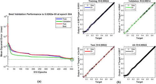
Table 6. ANN data and errors for n-propyl alcohol.

Q (m^3/h)	H (m)	NPSHr (m)	Pm (kW)	Torque (N.m)	Efficiency	Predicted efficiency	Error
0	89.76028	0.895765	5.5000	17.8942	0.003933	0.046984	−0.04305
2	89.76335	0.895765	5.7330	18.6523	0.074859	0.057599	0.017261
4	89.77258	0.895765	5.9660	19.4103	0.142479	0.142943	−0.00046
6	89.78797	0.895765	6.1990	20.1684	0.203876	0.208126	−0.00425
8	89.80951	0.895765	6.4320	20.9265	0.259889	0.260627	−0.00074
10	89.83721	0.895765	6.6650	21.6845	0.311214	0.312703	−0.00149
12	89.87106	0.895765	6.8980	22.4426	0.358433	0.357698	0.000736
14	89.91107	0.895765	7.1310	23.2007	0.40204	0.402733	−0.00069
16	89.95723	0.895765	7.3640	23.9587	0.442452	0.442626	−0.00017
18	90.00955	0.895765	7.5970	24.7168	0.480027	0.478807	0.00122
20	90.06802	0.895765	7.8300	25.4748	0.515074	0.514018	0.001056
22	90.13264	0.895765	8.0630	26.2329	0.547857	0.547824	3.24e-05
24	90.20343	0.895765	8.2960	26.9910	0.578608	0.578703	−9.4e-05
26	90.28036	0.895765	8.5290	27.7490	0.607531	0.606637	0.000894
28	90.36346	0.895765	8.7620	28.5071	0.634801	0.633479	0.001322
30	90.4527	0.895765	8.9950	29.2652	0.660576	0.66198	−0.0014

When the data set of phenol was entered to ANN model MSE was close to zero (0.000248). Figure 7 shows validation performance and regression analysis graphs of phenol’s data set. Table 7 shows inputs, output, ANN estimations and errors for phenol. Best validation performance was 0.00011757 at epoch 66. R was 0.99648 and R² provided a prediction accuracy of 99.297% which is in an acceptable range of accuracy.

Figure 7. Results of ANN with phenol’s data set: Validation performance (a) Regression analysis graphics (b).

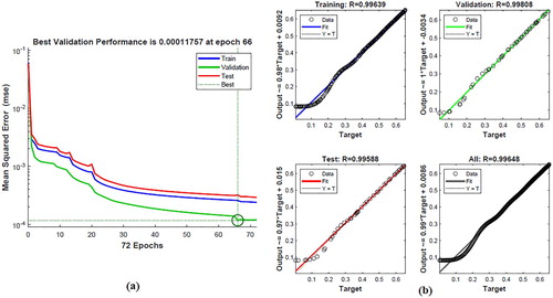
Table 7. ANN data and errors for phenol.

Q (m^3/h)	H (m)	NPSHr (m)	Pm (kW)	Torque (N.m)	Efficiency	Predicted efficiency	Error
0	66.13216	2.697194	5.5000	17.8942	0.003885	0.082168	−0.07828
2	66.13523	2.697194	5.7330	18.6523	0.073951	0.084396	−0.01045
4	66.14446	2.697194	5.9660	19.4103	0.140755	0.11129	0.029464
6	66.15985	2.697194	6.1990	20.1684	0.201421	0.188974	0.012447
8	66.18139	2.697194	6.4320	20.9265	0.256782	0.274161	−0.01738
10	66.20909	2.697194	6.6650	21.6845	0.307526	0.316272	−0.00875
12	66.24294	2.697194	6.8980	22.4426	0.354234	0.352725	0.001509
14	66.28295	2.697194	7.1310	23.2007	0.397393	0.401195	−0.0038
16	66.32911	2.697194	7.3640	23.9587	0.437418	0.442226	−0.00481
18	66.38142	2.697194	7.5970	24.7168	0.474665	0.475872	−0.00121
20	66.43989	2.697194	7.8300	25.4748	0.509437	0.5106	−0.00116
22	66.50452	2.697194	8.0630	26.2329	0.541999	0.544792	−0.00279
24	66.5753	2.697194	8.2960	26.9910	0.572582	0.57489	−0.00231
26	66.65223	2.697194	8.5290	27.7490	0.601385	0.601939	−0.00055
28	66.73532	2.697194	8.7620	28.5071	0.628584	0.628849	−0.00026
30	66.82457	2.697194	8.9950	29.2652	0.654335	0.654505	−0.00017

When the data set of chloroform was run with the ANN model, the MSE value was close to zero (1.39e-5). Figure 8 indicates, the validation performance and regression analysis graphs of chloroform’s data set. Table 8 illustrates inputs, the output, ANN estimations and errors for chloroform. Best validation performance was 2.9094e-5 at epoch 974. R was 0.99979 and R² provided a prediction accuracy of 99.958% R² which is in an acceptable accuracy for these kinds of applications.

Figure 8. Results of ANN with chloroform’s data set: Validation performance (a) Regression analysis graphics (b).

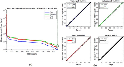
Table 8. ANN data and errors for chloroform.

Q (m^3/h)	H (m)	NPSHr (m)	Pm (kW)	Torque (N.m)	Efficiency	Predicted efficiency	Error
0	46.99481	6.370920704	5.5000	17.8942	0.003814	0.034054	−0.03024
2	46.99788	6.370920703	5.7330	18.6523	0.072588	0.064389	0.008199
4	47.00711	6.370920693	5.9660	19.4103	0.138168	0.138181	−1.3e-05
6	47.0225	6.370920654	6.1990	20.1684	0.197739	0.198378	−0.00064
8	47.04404	6.370920553	6.4320	20.9265	0.252121	0.251301	0.00082
10	47.07175	6.370920348	6.6650	21.6845	0.301996	0.30204	−4.4e-05
12	47.1056	6.370919985	6.8980	22.4426	0.347936	0.348701	−0.00076
14	47.14562	6.3709194	7.1310	23.2007	0.390424	0.38957	0.000853
16	47.1918	6.370918516	7.3640	23.9587	0.429868	0.429489	0.000379
18	47.24415	6.370917246	7.5970	24.7168	0.466621	0.467352	−0.00073
20	47.30266	6.370915491	7.8300	25.4748	0.500983	0.50133	−0.00035
22	47.36733	6.37091314	8.0630	26.2329	0.533215	0.532592	0.000624
24	47.43818	6.370910069	8.2960	26.9910	0.563545	0.562997	0.000547
26	47.5152	6.370906144	8.5290	27.7490	0.59217	0.592655	−0.00049
28	47.5984	6.370901215	8.7620	28.5071	0.619264	0.620014	−0.00075
30	47.68778	6.370895119	8.9950	29.2652	0.644981	0.643199	0.001782

When the data set of castor oil is run with the ANN model, the MSE value was close to zero (0.000129). Figure 9 illustrates validation performance and regression analysis graphs of castor oil’s data set. Table 9 indicates inputs, the output, ANN estimations and errors for chloroform. Best validation performance was 0.00016536 at epoch 194. R was 0.99812 and R² provided an acceptable prediction accuracy of 99.624%.

Figure 9. Results of ANN with castor oil’s data set: Validation performance (a) Regression analysis graphics (b).

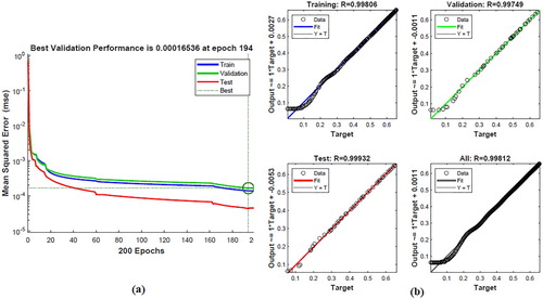
Table 9. ANN data and errors for castor oil.

Q (m^3/h)	H (m)	NPSHr (m)	Pm (kW)	Torque (N.m)	Efficiency	Predicted efficiency	Error
0	74.6542380	1.90748640	5.5000	17.8942	0.003906	0.06324	−0.05933
2	74.6573077	1.90748640	5.7330	18.6523	0.074342	0.067742	0.0066
4	74.6665399	1.90748640	5.9660	19.4103	0.141497	0.114064	0.027433
6	74.6819269	1.90748640	6.1990	20.1684	0.202478	0.211519	−0.00904
8	74.7034687	1.90748640	6.4320	20.9265	0.25812	0.262661	−0.00454
10	74.7311653	1.90748640	6.6650	21.6845	0.309114	0.305272	0.003842
12	74.7650167	1.90748640	6.8980	22.4426	0.356043	0.359415	−0.00337
14	74.8050229	1.90748640	7.1310	23.2007	0.399394	0.399441	−4.6E-05
16	74.8511839	1.90748640	7.3640	23.9587	0.439586	0.440533	−0.00095
18	74.9034997	1.90748640	7.5970	24.7168	0.476974	0.479049	−0.00207
20	74.9619703	1.90748640	7.8300	25.4748	0.511864	0.512669	−0.0008
22	75.0265957	1.90748640	8.0630	26.2329	0.544522	0.545208	−0.00069
24	75.0973759	1.90748640	8.2960	26.9910	0.575177	0.576749	−0.00157
26	75.1743109	1.90748640	8.5290	27.7490	0.604031	0.605687	−0.00166
28	75.2574007	1.90748640	8.7620	28.5071	0.631261	0.631976	−0.00071
30	75.3466453	1.90748640	8.9950	29.2652	0.657023	0.658899	−0.00188

When the data set of nitric acid is run with the ANN model, the MSE value was close to zero (4.26e-5). Figure 10 illustrates validation performance and regression analysis graphs of nitric acid’s data set. Table 10 shows inputs, the output, ANN estimations and errors for chloroform. Best validation performance was 5.332e-9 at epoch 5. R was 0.99934 and R² provided an acceptable prediction accuracy of 99.86%.

Figure 10. Results of ANN with nitric acid’s data set: Validation performance (a) Regression analysis graphics (b).

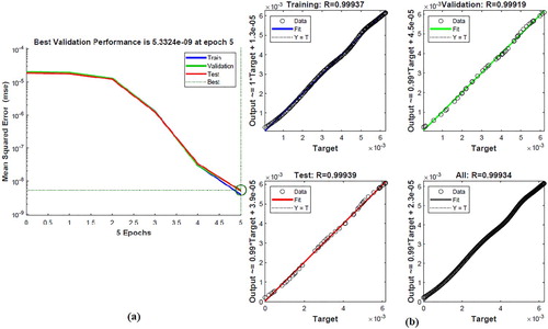
Table 10. ANN data and errors for nitric acid.

Q (m^3/h)	H (m)	NPSHr (m)	Pm (kW)	Torque (N.m)	Efficiency	Predicted efficiency	Error
0	50.8178201	5.1234506	5.5000	17.8942	0	0.021788	−0.02178849
2	50.8209943	5.1234261	5.7330	18.6523	0.06469	0.065637	−0.0009466
4	50.8305169	5.1233528	5.9660	19.4103	0.124351	0.117695	0.00665609
6	50.8463878	5.1232307	6.1990	20.1684	0.179571	0.175008	0.00456305
8	50.8686072	5.1230597	6.4320	20.9265	0.230856	0.232528	−0.0016717
10	50.8971749	5.1228398	6.6650	21.6845	0.278638	0.284768	−0.00613006
12	50.932091	5.1225711	6.8980	22.4426	0.323293	0.328346	−0.00505250
14	50.9733556	5.1222536	7.1310	23.2007	0.365147	0.363856	0.00129138
16	51.0209685	5.1218871	7.3640	23.9587	0.404485	0.396371	0.00811348
18	51.07493	5.1214718	7.5970	24.7168	0.441555	0.433736	0.00781915
20	51.1352398	5.1210077	7.8300	25.4748	0.47658	0.478396	−0.00181619
22	51.2018982	5.1204946	8.0630	26.2329	0.509752	0.519282	−0.00952990
24	51.2749051	5.1199328	8.2960	26.9910	0.541246	0.548154	−0.00690784
26	51.3542605	5.119322	8.5290	27.7490	0.571214	0.571075	0.00013852
28	51.4399644	5.1186624	8.7620	28.5071	0.599795	0.594202	0.00559293
30	51.5320169	5.1179539	8.9950	29.2652	0.627111	0.615326	0.011785243

The results of the ANN model illustrated that the efficiency predictions were performed with an acceptable margin of error. The network provided the close error values for each data set, and MSE values were close to zero. R² values are also close to 1 for each chemical. These outputs indicated satisfactory predictions of the model.

4. Conclusion

The results of the Simulink Model showed that when the pump handles the fluid with lower density than the density of the reference fluid, the head and the efficiency of the pump increases. Furthermore, dense fluids caused to drop the head markedly. NPSHr value increased with increased density. When the pump handled a viscous fluid, NPSHr decreased, and the head pump increased compared to less viscous fluids with close densities. While the vapour pressure of the fluid increased its viscosity also decreased so, the same outputs were valid for handling a viscous fluid in the pump. ANN application illustrated that the efficiency estimation can be achieved with recorded operation data. These data are recorded in the ship and may be obtainable for technical departments of shipping companies. The terminals also monitor these data. Using this kind of information can be important during the construction of a chemical tanker. Predictions with different fluids can provide safer and more efficient cargo operations. Besides, they can save money because of low defect rate of cargo pump.

Results of the ANN illustrated that, the network predicted the efficiency power MSE of the best prediction was very close to zero (1.1817e-6) and R² of the best prediction provided a prediction accuracy of 99.996%. Efficiency estimations of six other data sets have satisfactory R² and MSE values. The ANN model successfully predicted the efficiencies; thus, it is a useful method for this kind of application.

There are some limitations to this study. These can be listed as follows:

• In the study, it was desired to model a centrifugal pump that directly works as a cargo transfer pump on a chemical tanker, but data could not be obtained as excepted. Achieving the real operation data requires a long data acquisition process during the cargo transfer operation onboard. Furthermore, obtaining practicable data requires highly sensitive measurements. The model was created by obtaining the data, from a factory of a pump that is suitable for the ship and operated with different chemicals regarding size and capacity. The data is obtained by the Simulink Model numerically.

• In ANNs involved in efficiency estimation, there is no definite way to determine the proper network structure. Therefore, the general structure of the network is found by various trials. Fixed functions and values in MATLAB Neural Network Fitting Tool were used as they are in the software.

• The gauge pressures from the operation data were modelled by calculating the mean gauge pressures for each fluid in the Simulink model.

The recommendations for the further studies are listed below;

• Although ANNs are successful in predicting, they are not considered to be accurate results. Other methods for estimating can be used with this method for more successful estimates.

• The centrifugal pump data used in the research can be modelled directly by obtaining it from a ship and the criteria, which can vary according to ship’s conditions.

• Instead of using numerical data, optimisation studies can be performed with the operational data taken from the experiment sets or the running systems themselves.

• In addition to the centrifugal pump, a similar investigation can be conducted to other types of pumps or systems used in ships can be selected instead of estimating other extensions related to ANNs of the MATLAB program. Optimisation studies can be carried out with different methods and algorithms. Several software tools well accepted in the literature, can be used instead of MATLAB. Moreover, the researcher can write his/her own algorithm with different programming languages for optimisation studies.

Disclosure statement

No potential conflict of interest was reported by the authors.

ORCID

Onur Yüksel http://orcid.org/0000-0002-5728-5866

Correction Statement

This article has been republished with minor changes. These changes do not impact the academic content of the article.

References

- Allen DM. 1971. Mean square error of prediction as a criterion for selecting variables. Technometrics. 13(3):469–475. doi: 10.1080/00401706.1971.10488811
- An Z, Zhounian L, Peng W, Linlin C, Dazhuan W. 2016. Multi-objective optimization of a low specific speed centrifugal pump using an evolutionary algorithm. Eng Optim. 48(7):1251–1274. doi: 10.1080/0305215X.2015.1104987
- Armstrong JS, Collopy F. 1992. Error measures for generalizing about forecasting methods empirical comparisons. Int J Forecast. 8(1):69–80. doi: 10.1016/0169-2070(92)90008-W
- Azadeh A, Ebrahimipour V, Bavar P. 2010. A fuzzy inference system for pump failure diagnosis to improve maintenance process: The case of a petrochemical industry. Expert Syst Appl. 37(1):627–639. doi: 10.1016/j.eswa.2009.06.018
- Azadeh A, Saberi M, Kazem A, Ebrahimipour V, Nourmohammadzadeh A, Saberi Z. 2013. A flexible algorithm for fault diagnosis in a centrifugal pump with corrupted data and noise based on ANN and support vector machine with hyper-parameters optimization. Appl Soft Comput. 13(3):1478–1485. doi: 10.1016/j.asoc.2012.06.020
- Bachus L, Custodio A. 2003. Know and understand centrifugal pumps. Oxford: Elsevier. ISBN-13: 978-1856174091.
- Benini E, Cenzon M. 2009. Calibration of a meanline centrifugal pump model using evolutionary algorithms. J Power Energy. 223(7):835–847. doi: 10.1243/09576509JPE742
- Bluman AG. 2000. Elementary statistics. New York: McGraw Hill.
- Derakhshan S, Bashiri M. 2018. Investigation of an efficient shape optimization procedure for centrifugal pump impeller using eagle strategy algorithm and ANN (case study: slurry flow). Struct Multidiscipl Optim, 1-15.
- Derakhshan S, Pourmahdavi M, Abdolahnejad E, Reihani A, Ojaghi A. 2013. Numerical shape optimization of a centrifugal pump impeller using artificial bee colony algorithm. Comput Fluids. 81:145–151. doi: 10.1016/j.compfluid.2013.04.018
- Dreyfus G. 2005. Neural networks: methodology and applications. Berlin: Springer Science & Business Media.
- Durmusoglu Y, Kocak G, Deniz C, Zincir B. 2015. Energy efciency analysis of pump systems in a ship power plant and a case study of a container ship. Opatija: IAMU 16th AGA.
- Ertoz Ö. 2003. Energy efficiency in pumps. In: 6th National Installations Engineering and Congress; Istanbul.
- IMO. 2016. International code for the construction and equipment of ships carrying dangerous chemicals in bulk (IBC Code), 2016 Edition (ID100E), ISBN 978-92-801-1595-6 (9789280115956).
- Kaya D, Yagmur EA, Yigit KS, Kilic FC, Eren AS, Celik C. 2008. Energy efficiency in pumps. Energy Convers Manage. 49(6):1662–1673. doi: 10.1016/j.enconman.2007.11.010
- Khataee AR, Kasiri MB. 2010. Artificial neural networks modeling of contaminated water treatment process by homogeneous and heterogeneous nanocatalysis. J Mol Catal A: Chem. 331, 86–100. doi: 10.1016/j.molcata.2010.07.016
- Kocak G, Durmusoglu Y. 2017. Energy efficiency analysis of a ship’s central cooling system using variable speed pump. J Marine Eng Technol. DOI:10.1080/20464177.2017.1283192.
- Köseoğlu B. 2015. Port modeling and applying optimization techniques (book in Turkish). İzmir: Dokuz Eylul University.
- Lomakin VO, Chaburko PS, Kuleshova MS. 2017. Multi-criteria optimization of the flow of a centrifugal pump on energy and vibroacoustic characteristics. Procedia Eng. 176:476–482. doi: 10.1016/j.proeng.2017.02.347
- Makridakis S, Wheelwright S, Hyndman R. 1998. Forecasting methods and applications. 3rd edn. New York, NY: Wiley.
- Mathworks. 2018. Simulation and model-based design, [accessed 2017 October 22]. https://www.mathworks.com/products/simulink.html.
- Najafi A, Nowruzi H, Ghassemi H. 2018. Performance prediction of hydrofoil-supported catamarans using experiment and ANNs. Appl Ocean Res. 75:66–84. doi: 10.1016/j.apor.2018.02.017
- Nourbakhsh A, Safikhani H, Derakhshan S. 2011. The comparison of multi-objective particle swarm optimization and NSGA II algorithm: applications in centrifugal pumps. Eng Optim. 43(10):1095–1113. doi: 10.1080/0305215X.2010.542811
- Nowruzi H, Ghassemi H, Ghiasi M. 2017. Performance predicting of 2D and 3D submerged hydrofoils using CFD and ANNs. J Mar Sci Technol. 22(4):710–733. doi: 10.1007/s00773-017-0443-0
- Olszewski P. 2016. Genetic optimization and experimental verification of complex parallel pumping station with centrifugal pumps. Appl Energy. 178:527–539. doi: 10.1016/j.apenergy.2016.06.084
- Oztemel E. 2016. Artificial neural networks (book in Turkish). 4th ed. İstanbul: Ozkaracan Publishing, Papatya Bilim.
- Pillon LZ. 2007. Interfacial properties of petroleum products. Boca Raton, FL: CRC Press.
- Sakar C, Zorba Y. 2013. Operational efficiency at chemical tankers (book in Turkish). İstanbul: Beta Publishing.
- Sakthivel NR, Nair BB, Sugumaran V. 2012. Soft computing approach to fault diagnosis of centrifugal pump. Appl Soft Comput. 12(5):1574–1581. doi: 10.1016/j.asoc.2011.12.009
- Sakthivel NR, Sugumaran V, Babudevasenapati S. 2010. Vibration based fault diagnosis of monoblock centrifugal pump using decision tree. Expert Syst Appl. 37(6):4040–4049. doi: 10.1016/j.eswa.2009.10.002
- Shora MM, Ghassemi H, Nowruzi H. 2018. Using computational fluid dynamic and artificial neural networks to predict the performance and cavitation volume of a propeller under different geometrical and physical characteristics. J Marine Eng Technol. 17(2):59–84. doi: 10.1080/20464177.2017.1300983
- Su Z, Tang B, Liu Z, Qin Y. 2015. Multi-fault diagnosis for rotating machinery based on orthogonal supervised linear local tangent space alignment and least square support vector machine. Neurocomputing. 157:208–222. doi: 10.1016/j.neucom.2015.01.016
- Taghva HR, Ghassemi H, Nowruzi H. 2018. Seakeeping performance estimation of the container ship under irregular wave condition using artificial neural network. Am J Civil Eng Architecture. 6(4):147–153. doi: 10.12691/ajcea-6-4-3
- Wang C, Shi W, Wang X, Jiang X, Yang Y, Li W, Zhou L. 2017. Optimal design of multistage centrifugal pump based on the combined energy loss model and computational fluid dynamics. Appl Energy. 187:10–26. doi: 10.1016/j.apenergy.2016.11.046
- Wu P, Lai Z, Wu D, Wang L. 2014. Optimization research of parallel pump system for improving energy efficiency. J Water Res Planning Manage. 141(8):04014094. doi: 10.1061/(ASCE)WR.1943-5452.0000493
- Yumurtaci Z, Sarıgul A. 2011. Energy efficiency of centrifugal pumps and its applications (paper in Turkish). Makina Mühendisleri Odası Tesisat Mühendisliği Dergisi. 122:49–58.