Post stack seismic data processing for enhancing subsurface reservoir mapping in the Shushan basin, Western Desert, Egypt

ABSTRACT

Reprocessing of seismic reflection data over Nader field in the Egyptian Western Desert, improved the images of the surface structural framework. The appearance of seismic data can be affected by various factors apart from subsurface structure, including data acquisition problems and processing artefacts. Different post-stack processing steps were tested and compared to the original seismic data determine the enhancement of data quality and improvements on imaging the subsurface. The applied post-stack processing sequence increased the seismic data resolution through increasing the signal-to-noise ratio, enhancing faults detection, and reflectors sharpness and continuity. The Time Variant Frequency Filter (TVF) application is found to be better than applying the filter in one time window and provided more detailed frequency contents and in turn better reflectors identification. The Frequency/Wave Number (F/K) filter removed lot of the existing linear noises resulted in more clear images. The Frequency/Distance (F/X) Deconvolution enhanced the data coherency by removing the existing random noises. The Spiking Deconvolution showed remarkable enhancement in compressing the reflectors and increasing their continuity. The reprocessed data interpretation of Abu Roash C member in Nader Filed, Shushan basin, North Western Desert, Egypt, comparing to the original, showed better mapping and faults detection, which highlighted new potential structures that could act as hydrocarbon traps.

KEYWORDS:

• Post-stack processing
• data quality enhancement
• seismic resolution Shushan basin
• Western desert

1. Introduction

Seismic reflection data usually contains signal and noises. Other than the fundamental reflections from the underlying layers, noises encompass all unwanted energy. Seismic purity in depicting the subsurface image is substantially harmed by noise. Noise can be efficiently decreased by intentional efforts during data processing and reprocessing, even though it is normally undesirable. It is usual practice to evaluate data quality in terms of a signal-to-noise ratio (S/N).

Seismic data processing involves a series of sequential processes, each with various approaches that can be applied. Certain approaches are applied solely before stacking, while others are used both before and after stacking. In this study, the post-stack processing sequence was evaluated and presented since pre-stack seismic data was unavailable.

Post-stack reprocessing can improve the resolution of seismic data, resulting in clearer images of subsurface structures. This enhancement in image quality can assist geologists and engineers in making more precise interpretations of subsurface geology and reservoir properties. The main objective of this study is to evaluate the structural style and primary stratigraphic horizons in Nader field by utilising available 2D seismic data, along with advanced analysis and interpretation of the seismic and well data. Additionally, this study aims to examine the potential for improving seismic data quality through reprocessing, which would enhance the signal-to-noise ratio of the seismic data.

2. Geological setting

Nader Field is found in the North Western Desert, in the Shushan basin’s south western section, between 30° 34’40“and 30° 32’ 40” N and 26° 57’36“and 26° 55’ 12” E (Figure 1).

Figure 1. (a) location map of the Nader oil field at the southwestern part of Shushan basin (modified after Egyptian General Petroleum Corporation (EGPC) 1992) and (b) Base map for 20 seismic lines that uses in this study.

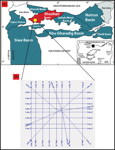
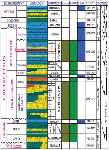
The Shushan Basin, which is the largest of the coastal basins, is classified as a half-graben system and comprises Jurassic to Palaeogene sediments with a maximum thickness (El Shazly 1977; Hantar 1990). Abdel-Fattah et al. (2019) considered Shushan basin as a largest tight gas sand reserve in northwestern Africa. The sedimentary section of this basin ranges from the Lower Palaeozoic to Recent and covers a wide range of sedimentary environments (Figure 2) El-Dabaa et al. (2022) used the Artificial Intelligence (AI) algorithms for seismic reservoir characterisation of Nader field.

Figure 2. Generalized stratigraphic nomenclature, northern Western Desert including Shushan basin, Egypt and the red box refers to the interested Member (Abu Roash-C) (modified after Bevan and Moustafa 2012; Shalaby et al. 2013).

The structural features of the northwestern Desert, including the Shushan Basin, were primarily formed by vertical movements of basement blocks, resulting in draped over and/or faulted anticline features. Compressional anticlines, on the other hand, are subordinate and are likely formed by drag folding associated with lateral movements along basement faults. The predominant structures in the northwestern Desert, specifically the Shushan Basin, consist of parallel, elongated, tilted fault blocks, i.e. horst and half-graben structures, which have led to erosion of the upthrown blocks (Barakat 2017).

3. Data and methodology

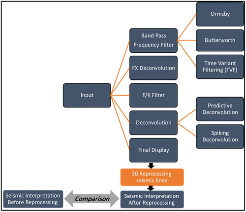
The input data consists of 20 pre-stack time migrated stacked seismic sections in time that undergone generally the following processing flow: Noise Attenuation, Scaling, Deconvolution, Static corrections, Migration, Multiple Elimination, Stack, Deconvolution, TV Filter, Zero Phasing, and Trim Statics. The workflow used in the current research is depicted in the presented diagram (Figure 3). The applicable workflow includes the Bandpass filter (BPF), spatial predictive deconvolution in the complex frequency domain (FX deconvolution), frequency – wave number (F/K) filter, predictive and spiking deconvolution. The applied post-stack processing sequence increased the seismic data resolution through increasing the signal-to-noise ratio, enhancing faults detection, and reflectors sharpness and continuity.

Figure 3. The general workflow used in the present study.

After the CDP gathering, some procedures can be applied to improve the interpretability of the final seismic section. Extensive testing of numerous processing steps and parameters only gradually improved the data quality. Deconvolution, random noise attenuation and migration with optimal parameters can be used (Leaf et al. 1996). In order to represent any waveform in terms of its distinct sine wave components, it is important to define not only the frequency of each element but also its amplitude and phase (Kearey et al. 2002). The reflection seismic, two-dimensional, or three-dimensional (2D or 3D), represents the most accurate tool for the structural definition and relations between layers of subsurface geology in sedimentary basins (Amorim et al. 2019). If ambient noise is very low, a layer with a thickness of 1/40 of the seismic wavelength can theoretically be detected (Sun et al. 2020).

In order to differentiate between signal and noise components of the data, it is important to analyse the frequency, amplitude, and phase. Therefore, the data can be represented in two different ways. A known time domain, in which the amplitude of a wave is expressed as a function of time, or frequency domain, in which the amplitude and phase of an individual sine wave are represented as a function of frequency.

3.1. Frequency filter

In seismic data processing, filtering is a technique for limiting the frequency content of an initial signal (Latiff et al. 2016). A frequency filter is a signal processing step that changes the amplitude and, in certain cases, phase of a seismic signal in relation to frequency. Filters are used in a variety of applications to highlight signals in a certain frequency band while rejecting or suppressing signals in the unwanted frequency range. The cut-off frequency is the frequency that separates the attenuation band from the pass.

There are distinctive categories of filters based on their operation, Butterworth and Ormsby are the well-known sorts. Filters can apply to cut or pass either lowest or highest frequencies, as low cut/high pass, low pass/high cut, or band-pass, and they either apply to the total length of the seismic section (one window) or differ at different time windows (time variation filter; TVF).

The slopes of a band-pass filter indicate how much a frequency outside of the passband is decreased by the filter. The slopes can be defined in two ways: by specifying amplitude values for four distinct frequencies, or by specifying it as a taper (Butterworth and Ormsby Band-pass Filters), that is, by specifying how much dB per octave (Yan and Li 2019).

Several tests using all types of filters were tried. Because the results of the Butterworth and Ormsby filter tests were nearly identical, the authors chose to focus on the Ormsby filter application examples in this work (Figures 4–6).

Figure 4. Line # 1 amplitude spectrum and BPF designs: (a) Butterworth BPF low F: 6 Hz, high F: 31, low Slope: 18 dB/oct., & high Slope: 72 dB/oct and (b) Ormsby BPF low Cut: 6 Hz, low pass: 12 Hz, high pass: 28 Hz, & high Cut: 34 Hz.

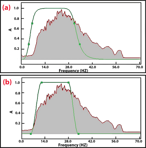
Figure 5. Line # 1 band pass filter (BPF) test: 2-5-10-20 Hz showing the harsh effects, especially on the high frequency contents. (a) before BPF application, (b) after BPF application, (c) difference (after – before), &; (d) amplitude spectrum after BPF application.

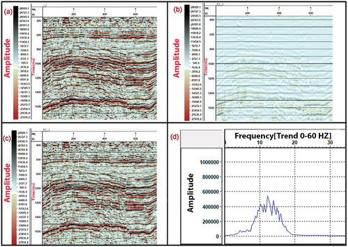
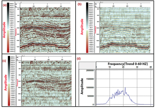
Figure 6. Line # 1 band pass filter (BPF) test: 2-5-20-30 Hz. This test showed the harm effect on the high frequency contents, especially at time windows of (900 to 1300 ms) and also in (500 to 650 ms). (a) before BPF application, (b) after BPF application, (c) difference (after – before), & (d) amplitude spectrum after BPF application.

On the existing data, the effect of the various types of filters stated above was investigated, and the Ormsby time-variant filter was determined to produce the best results (Figure 7). This is most likely due to the data’s amplitude spectrum narrowing over time. Various parameters tests were conducted with various overlapping time windows in order to select the best parameters and proceed to the rest of the processing flow phases (Table 1).

Figure 7. Line # 1 band pass time variant filter (TVF) with the parameters mentioned in table 1. This test outperformed prior tests in terms of improving data quality and maintaining both low and high frequency content. (a) before TVF application, (b) after TVF application, (c) difference (after – before), & (d) amplitude spectrum after TVF application.

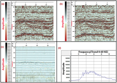
Table 1. The best test of Ormsby band-pass TVF.

Time	Low Truncation	Low Cut Freq.	High Cut Freq.	High Truncation
350–1300 ms	10	15	55	60
1200–1400 ms	5	10	40	50
1350–1700 ms	5	10	35	40
1650–1800 ms	5	10	30	40

3.2. FX deconvolution

The FX deconvolution is a spatial filtering process that enhances coherent data (regardless of dip) across a group of traces (Canales 1984). FX deconvolution begins by splitting the data into tiny enough windows to make events of interest appear linear. After that, the data in each window is Fourier converted. A prediction filter is constructed for each frequency and applied twice, once forward in space and once backwards. The inverse Fourier transform is applied to the two predictions, and the windows are blended back into the output. Each frequency’s operations are unaffected by those of other frequencies. This gives you a lot of leeway when it comes to predicting the outcome.

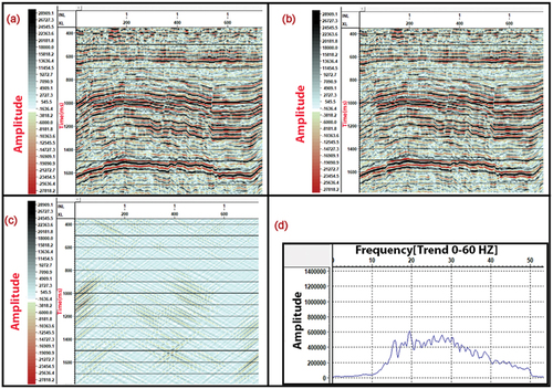
By altering the parameters of the FX deconvolution application window, the data under study was filtered to remove as much random noise as possible, and then they were tested (Table 2) to see which one produced a satisfactory result and was not harsh on the data. FX Deconvolution was used to improve the signal (coherent data) and reduce non-coherent noise (Figure 8).

Figure 8. Line # 1 FX deconvolution application; (a) before applying FX Decon. (b) after applying FX Decon.(c) difference (after – before), & (d) amplitude spectrum after FX Decon application.

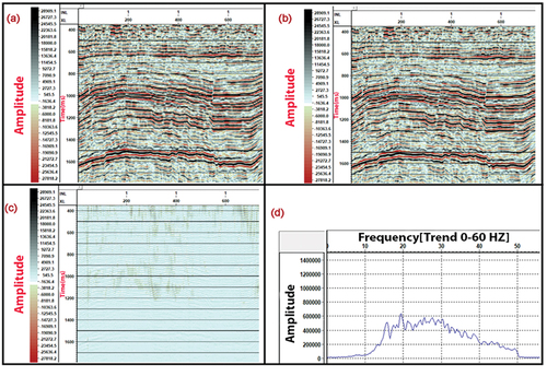
Table 2. The number of different tests from 001 to 006 for FX deconvolution.

Test	Filter Length	Design Window	Cut-off Freq.
001	1	100	50
002	3	100	60
003	3	100	50
004	3	150	50
005	7	100	50
006	3	100	40

3.3. F-K filter

F-K filtering is works in the frequency and wave number (F-K) domain, where the seismic data is filtered to remove the undesired frequencies higher and/or lower than the seismic signal band, and then sent back to the time-displacement domain. The procedure is a two-dimensional Fourier transformation and must be sampled according to the Nyquist criterion to avoid aliasing (Gigandet 2014).

Data had been transformed to the frequency by wave number domain (F-K) to check for dipping linear noise (Figure 9). This domain allows selection regions according to slope of events. Therefore, it becomes effective for linear noise attenuation. The resulting F-K filtered output data was cleaner, indicating an increase in the signal/noise ratio, as seen by the output minus input difference plot (Figure 10).

Figure 9. F-K spectrum design window for line #1 showing the noise regions that picked for attenuation.

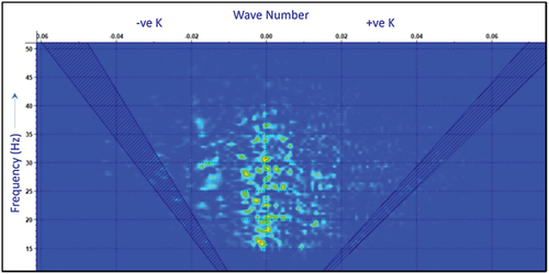
Figure 10. Line # 1 F-K application showing how much linear noises had been attenuated; (a) before applying F-K filter, (b) after applying F-K filter, (c) difference (after – before), & (d) amplitude spectrum after FX Decon application.

3.4. Deconvolution process

Deconvolution improves the visibility of tiny features in seismic data, as well as the clarity and interpretability of reflections (Onajite 2013). Deconvolution after stack is commonly used to recover high frequencies that have been attenuated by CMP stacking. It can also be used to reduce reverberations and multiples with short periods of time (Yilmaz 2001). Deconvolution can be predictive or spiking, in practice, both forms perform a mixture of wavelet compression and de-reverberation (Bacon et al. 2003). The predicted component of the seismic trace (multiple reflections) is removed in predictive deconvolution, while the unexpected component of the seismic trace (reflectivity series) is left unaltered (Onajite 2013).

In spiking deconvolution, by reducing the wavelet to a spike, we are effectively convolving a spike (the wavelet) with a sequence of spikes (the reflectivity series), yielding the intended output – a spiked seismic trace equal to the reflectivity series (Robinson and Saggaf 2001).

Post-stack deconvolution is considered for two main expectations, the presence of a residual wavelet on the stacked section and the presence of short period multiples. High frequencies have been recovered, multiples have been attenuated, amplitudes have been equalised, and a zero-phase wavelet has been produced via the post-stack deconvolution. Both predictive and spiking techniques were tested with different parameters (Tables 3 and 4). The remaining multiple reflections were suppressed, the wavelet form and amplitude spectrum of the input data were adjusted, and the resolution was somewhat boosted using predictive deconvolution (Figures 11 and 12). The temporal resolution was improved by spiking deconvolution, which compressed the wavelet and improved the sharpness and continuity of the reflectors (Figures 13 and 14).

Figure 11. Line # 1 predictive deconvolution application showing important improvement in vertical resolution as it can be verified by the Autocorrelation plot. Short period multiples had been attenuated, the wavelet is compressed further, and the reflectors are better characterised; (a) before applying predictive deconvolution (input), (b) Autocorrelation of the input that was used to choose deconvolution parameters (c) output after applying predictive deconvolution (OL = 240, gap = 32, PW = 1, DW = 0–2000), (d) Autocorrelation of the output that was used for evaluation.

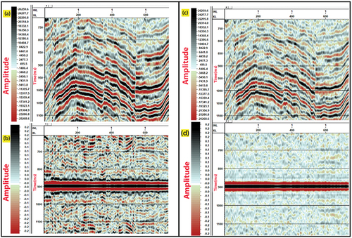
Figure 12. Line # 1 Average amplitude Spectra (a) before and (b) after applying the predictive deconvolution in Figure 16 (time window 700–1200 ms). The spectrum is flattened, albeit incompletely.

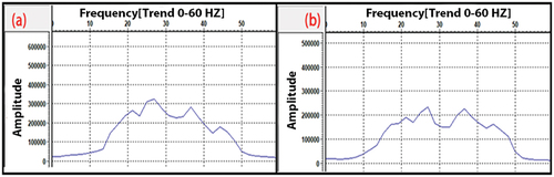
Figure 13. Line # 1 spiking deconvolution application showing significant improvement in the temporal resolution, including compress the wavelet and improved the sharpness and continuity of the reflectors.; (a) before applying spiking deconvolution (input), (b) Autocorrelation of the input (c) output after applying spiking deconvolution (OL = 20, PW = 1, DW = 300–1800), (d) Autocorrelation of the output that was used for evaluation.

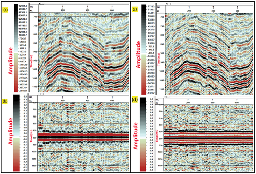
Figure 14. Line # 1 Average amplitude Spectra (a) before applying spiking deconvolution (input) and (b) after applying spiking deconvolution (output). The target of spiking deconvolution is to flatten the output spectrum, although the output spectrum nearly is flat (fig 19 b), it is far from representing a spike. The desired spike output can be obtained if the input is a minimum-phase wavelet, rather than a mixed-phase.

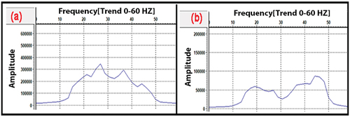
Table 3. Many tests for predictive deconvolution from 001 to 009 by changing in all parameters to remove the reverberation to check which one is the best.

Test	Operator Length	Pre-whitening	Lag	Design Window
001	240	1	32	0–2000
002	240	1	32	300–2000
003	240	1	32	500–2000
004	240	1	8	0–2000
005	240	1	12	0–2000
006	240	5	32	0–2000
007	240	10	32	0–2000
008	100	1	32	0–2000
009	160	1	32	0–2000

Table 4. Many tests for spiking deconvolution from 001 to 006 by changing of operator length and design window with the same number of pre-whitening for each test to spike the wavelet to reduce its effect then we compare between the result of predictive and spiking deconvolution to select which one is the perfect result to our final interpretation.

Test	Operator Length	Pre-whitening	Design Window
001	40	1	0–1800
002	40	1	300–1800
003	80	1	300–1800
004	120	1	300–1800
005	20	1	300–1800
006	10	1	300–1800

4. Post-processing structural mapping

High-quality structural maps have a lot to offer the oil and gas exploration. The capacity to make solid judgements about the size and geometry of a hydrocarbon trap, as well as how any reserves may be divided throughout compartments, is strongly influenced by the quality of such maps.

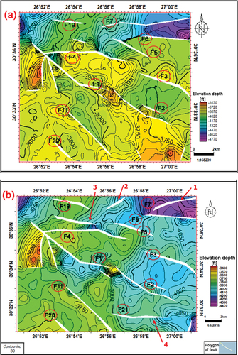
Following the completion of this post-stack processing workflow, re-interpretation for the whole seismic lines were performed to demonstrate the effect of processing on the interpretation (Figures 15 and 16) and mapping for the Abu Roash-C Member, one of the known reservoir sections in the study area, as shown in Figure 17 There are numerous differences between the depth map before and after post-stack techniques. For example, the depth ranges in both maps differ significantly. The values of map (a) range from −3570 to −4770 feet, while map (b) range from −3480 to −4470 feet. In addition, four major differences with faults were marked between map (a) and map (b) that are illustrated in red arrows in Figure 17: (1) Appeared as a separate fault running NE-SW, (2) shrank, revealing an un-faulted area to the north, and (3) grew longer (stretched), which could add area to a lead at its upthrown side, and (4) totally new EW fault which could add new leads (prospective area of 3-way dip closure).

Figure 15. (a) the whole section of line-1 with interpretation of horizons before applying any processing techniques and (b) the time window (650–1150 ms) of line to be clearer and focus on reflectors.

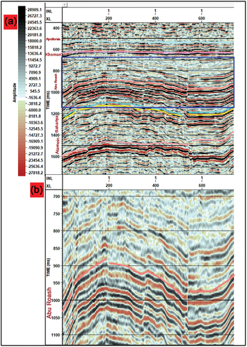
Figure 16. (a) the whole section of line-1 after applying the workflow of post stack processing and (b) the time window (650–1150 ms) of line to show the most difference was affected on reflectors especially around Abu Roash Formation. The horizons become more sharper, and some faults were shown.

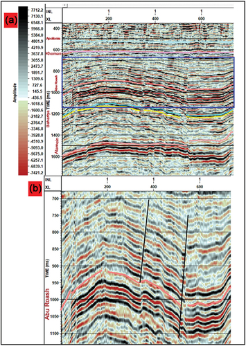
Figure 17. (a) the depth map of Abu Roash-C Member before applying any processing techniques on 20 seismic lines and (b) the map after applying the workflow of post-stack processing techniques on all seismic lines of study area.

5. Discussion

Numerous studies with different workflows have been conducted to enhance seismic imaging such as (Soliman et al. 2014; Munteanu et al. 2018; Abdel Fattah et al. 2020; Osinowo 2020). Several examples have demonstrated the production of clear subsurface images, even in the presence of diverse geological conditions and varying parameters for data acquisition and processing. Although each environment presents its unique challenges, the effectiveness of this method ultimately hinges on the quality of the final seismic images. These images constitute the principal basis for supporting geological interpretation and defining drilling targets (Bellefleur et al. 2018).

This research aims to determine the possibility for improving subsurface geological mapping using various seismic post-stack processing procedures. Several processing procedures were performed with various test parameters to find the best flow, which, according to the authors, increased seismic data quality, aided better interpretation, and improved created subsurface geological mapping. The chosen post-stack processing flow includes in sequence: Time Variant Band-Pass Frequency Filter (TVF), Frequency-Spatial predictive deconvolution (FX deconvolution), Frequency-Wave Number (F-K) filter, and Post-Stack Deconvolution.

The frequency content of the stack was evaluated for all studied seismic lines, and several filter parameters were tested. The results for Butterworth and Ormsby Band Pass Filter (BPF) are identical, and the testing revealed that each filter setting was applied to the entire section, enhancing data in some areas while being harsh in others, including the horizons of interest. On the other hand, the time-variant filter (TVF), which is a variation of the BPF and is applied through overlapping windows, is predicted. Parameters (Table 1) were found to provide the best data enhancement for tested lines out of all the tests performed. Figure 7 illustrates the result using one line as an example.

The FX deconvolution was then applied, and the following parameters: Filter length of 3 ms, design window of 100 ms, and Cut-off frequency of 50 HZ, were found to be the optimum for test line number 1 (Figure 8).

Therefore, the FK filter is applied to reduce the unwanted frequencies of the dipping linear noises, higher and/or lower than the seismic signal band Figure 8. The successful consequence of applying the F-K filter in removing the dipping noise from the data is seen in Figure 10 of line-1.

Post-stack deconvolution is then tested and applied using the selected optimum parameters (Tables 3 and 4). Both predictive and spiking techniques were tested. Predictive Deconvolution application (Figure 11) showed significant improvement in vertical resolution. Short period multiples had been attenuated, the wavelet is compressed further, the reflectors are better characterised, and the average amplitude spectrum is flattened, albeit incompletely. Test 001 gives the best result for predictive deconvolution for tested lines of parameters (OL = 240 ms, gap = 32 ms, PW = 1% and DW = 0–2000 ms).

Spiking Deconvolution application showed significant improvement in the temporal resolution, including compress the wavelet and improved the sharpness and continuity of the reflectors. The result is presented of how long the operator length is, spiking deconvolution in this case has failed to flatten the spectrum completely within the passband. According to the shortening operator length, the best tests are Test 005 of parameters (OL = 20, PW = 1, DW = 300–1800) (Figure 13).

The goal of spiking deconvolution is to flatten the output spectrum, although the output spectrum nearly is flat (Figure 14(b)), it is far from representing a spike. The desired spike output can be obtained if the input is a minimum-phase wavelet, rather than a mixed-phase. We compared the results obtained from the best performing predictive deconvolution and spiking deconvolution algorithms to determine which one yields better outcomes. Overall, our findings suggest that spiking deconvolution is a more effective technique for enhancing seismic data quality, particularly in applications where the identification of individual reflectors is crucial.

We performed re-interpretation for the entire seismic lines following the completion of the post-stack processing workflow to demonstrate the effect of processing on the generated seismic depth map, notably of one of the main reservoir sections in the research area, the Abu Roash-C Member. There were a lot of variations between the pre- and post-processing depth maps. The resulting map’s depth range changed significantly from −3480 to −4470 feet, whereas it was −3480 to −4470 feet before processing.

There were also significant variations in existing faults, such as fault orientations, the disappearance of some faults and the introduction of new ones, and the length of fault extension. By adding additional structural closures, these new structures may change the study area’s hydrocarbon potentiality.

6. Conclusion

This study revealed the benefits of employing post-stack seismic data processing to improve vintage seismic data. Increased signal-to-noise ratio, improved fault identification, and reflector sharpness and continuity are all advantages of post-stack processing. The application of a time variant filter is found to be superior to applying the filter in a fixed time window. Many of the current linear noises were removed by using the F-K filter. By reducing the existing random noises, the F/X Deconvolution improved data coherency. The Spiking Deconvolution demonstrated a significant improvement in compressing and enhancing the continuity of the reflectors. The data interpretation after reprocessing revealed improved mapping and fault detection, revealing new possible structures that could operate as hydrocarbon traps. In order to achieve the present improvement using post-stack processing, it is highly recommended to do pre-stack reprocessing beginning with field recorded seismic data, as this is likely to significantly increase data quality.

Acknowledgments

The authors are acknowledging the Egyptian General Petroleum Corporation (EGPC) and Khalda Petroleum Company for providing the necessary data and the permission to publish this study. The authors are also grateful to Schlumberger for granting access to the academic license of the software (Petrel and Vista seismic processing software) used in this study.

Disclosure statement

No potential conflict of interest was reported by the authors.

References

- Abdel Fattah TH, Diab A, Younes M, Ewida H. 2020. Improvement of Gulf of Suez subsurface image under the salt layers through re-processing of seismic data-a case study. NRIAG J Astron Geophys. 9(1):38–51. doi: 10.1080/20909977.2020.1711575.
- Abdel-Fattah TA, Rashed MA, Diab AI. 2019. Reservoir compartmentalization phenomenon for lower safa reservoir, obaiyed gas field, northwestern Desert, Egypt. Arab J Geosci. 12(22):1–13. doi: 10.1007/s12517-019-4853-7.
- Amorim F, Popoff L, Figueiredo P, Nogueira A. 2019. Why reprocess seismic data. Sixteenth Int Congress Brazilian Geophys Soc. 1–5. doi: 10.22564/16cisbgf2019.184.
- Bacon M, Simm R, Redshaw T. 2003. 3-D seismic interpretation. UK: Cambridge University Press. 212. doi: 10.1017/CBO9780511802416.
- Barakat MK. 2017. Petrophysical evaluation and potential capability of hydrocarbon generation of Jurassic and cretaceous source rocks in Shoushan basin, North Western Desert, Egypt. IOSR JAGG. 5(1):23–45. doi: 10.9790/0990-0501022345.
- Bellefleur G, Cheraghi S, Malehmir A 2018. Reprocessing legacy 3D seismic data from the halfmile lake and Brunswick no. 6 VMS deposits, New Brunswick, Canada.
- Bevan TG, Moustafa AR. 2012. Inverted rift-basins of northern Egypt. Elsevier.
- Canales L 1984. Random noise reduction: 54th Annual International Meeting, SEG, Expanded Abstracts: 525–527.
- Egyptian General Petroleum Corporation (EGPC). 1992. Western Desert oil and gas fields - a comprehensive overview. The Egyptian General Petroleum Corporation. pp. 30–34.
- El-Dabaa SA, Metwalli FI, Amin AT, Basheer AA. 2022. Prediction of porosity and water saturation using a probabilistic neural network for the bahariya formation, Nader field, north western desert, Egypt. J Afr Earth Sci. 196:104638. doi: 10.1016/j.jafrearsci.2022.104638.
- El Shazly EM. 1977. The geology of the Egyptian region. In: Nairn AEM, Kanes WH Stehli FG, editors. The ocean basins and margins. New York; pp. 379–444. doi: 10.1007/978-1-4684-3036-3_10.
- Gigandet KM. 2014. Processing and interpretation of Illinois basin seismic reflection data.
- Hantar G. 1990. North Western Desert. In: Said R, editor. The geology of Egypt. Balkema, Rotterdam; pp. 293–319. doi: 10.1201/9780203736678-15.
- Kearey P, Brooks M, Hill I. 2002. An introduction to geophysical exploration. 4. Blackwall Publishing company, USA: John Wiley & Sons.
- Latiff AA, Jamaludin SNF, Zakariah MNA. 2016. Post-stack seismic data enhancement of thrust-belt area, Sabah basin. IOP Conf Ser: Earth Environ Sci. 30(1):12006. IOP Publishing. doi: 10.1088/1755-1315/30/1/012006.
- Leaf GA, Ting SC, Fried JG, Young J, Van Dok RR. 1996. 3-D processing success of difficult seismic data in the Val Verde basin, Texas. In: SEG technical program expanded abstracts 1996. USA: Society of Exploration Geophysicists; pp. 1200–1203 doi: 10.1190/1.1826312.
- Munteanu I, Diviacco P, Sauli C, Dinu C, Burcă M, Panin N, Brancatelli G. 2018. New insights into the blacksea basin, in the light of the reprocessing of vintage regional seismic data. In: Diversity in coastal marine sciences: historical perspectives and contemporary research of geology, physics, chemistry, biology, and remote sensing. pp. 91–114. doi: 10.1007/978-3-319-57577-3_6.
- Onajite E. 2013. Seismic data analysis techniques in hydrocarbon exploration. USA: Elsevier.
- Osinowo OO. 2020. Reprocessing of regional 2D marine seismic data of part of Taranaki basin, New Zealand using Latest processing techniques. GeoSci Eng. 66(2):95–116. doi: 10.35180/gse-2020-0035.
- Robinson EA, Saggaf M. 2001. Klauder wavelet removal before vibroseis deconvolution. Geophys Prospect. 49(3):335–340. doi: 10.1046/j.1365-2478.2001.00260.x.
- Shalaby MR, Hakimi MH, Abdullah WH. 2013. Modelling of gas generation from the Alam El-Bueib formation in the Shoushan basin, northern Western Desert of Egypt. Int J Earth Sci. 102(1):319–332. doi: 10.1007/s00531-012-0793-0.
- Soliman K, Ewida HF, Maher G 2014. Re-processing of 2D seismic data from razzak oil field, Western Desert, Egypt.
- Sun R, Kaslilar A, Juhlin C. 2020. Reprocessing of high-resolution seismic data for imaging of shallow groundwater resources in glacial deposits, SE Sweden. Near Surf Geophys. 18(5):545–559. doi: 10.1002/nsg.12101.
- Yan Y, Li QM. 2019. Low-pass-filter-based shock response spectrum and the evaluation method of transmissibility between equipment and sensitive components interfaces. Mech Syst Signal Process. 117:97–115. doi: 10.1016/j.ymssp.2018.07.023.
- Yilmaz Ö. 2001. Seismic data analysis. Tulsa: Society of Exploration Geophysicists exploration geophysicists. 1809. doi: 10.1190/1.9781560801580.