Integrated GPR analysis and numerical modelling for discovering archaeological mysteries at Kom Ombo temple

ABSTRACT

Archaeological research is made accurate and detailed by non-invasive geophysical techniques. Hence, the thorough utilisation of GPR data sets alongside numerical modelling is imperative for reducing uncertainty surrounding archaeological sites. This study aims to assess the practicality and efficacy of GPR numerical modelling in analysing concealed archaeological elements within the renowned Kom Ombo temple in southern Egypt. Using 80 MHz and 270 MHz antennas to detect any buried structures on the temple grounds. From the processed 2D GPR sections, two distinct anomalies (deep and shallow) were identified, possibly indicating hidden archaeological structures. Given the likelihood of these features possessing complex geometries, four synthetic models were devised, maintaining consistent electrical properties while varying in buried body geometry, to evaluate the GPR response. Convolution perfectly matched layer (CPML) absorbing media was designed to absorb waves within the modelling grid, alongside a transverse magnetic (TM) mode formulation, were utilised. The findings suggest that the deep anomaly could potentially represent a tunnel or significant geological formation, while the shallow anomaly may correspond to an extension of the Turkish fort. Overall, numerical modelling emerges as an enhanced mapping tool for uncovering hidden archaeological features in areas worldwide where excavation via traditional methods is not feasible.

KEYWORDS:

• Kom Ombo temple
• GPR survey
• hidden archaeological structures
• synthetic models
• convolution perfectly matched layer (CPML)
• transverse magnetic mode (TM)

1. Introduction

Ground Penetrating Radar (GPR) stands out as a commonly used non-destructive technique, offering a comprehensive view of subsurface structures with high spatial resolution, capable of reaching depths from centimetres to tens of metres. Employing antennas spanning frequencies from 10 MHz to 2.6 GHz, GPR serves diverse purposes in fields such as construction, archaeology, geophysics, and engineering (Reynolds 2011). However, complexities within GPR data can potentially lead to misinterpretation, prompting the utilisation of validation approaches like numerical modelling. Various methods, including ray-based, frequency-domain, integral, and Finite Difference Time Domain (FDTD) techniques, have been developed for GPR numerical modelling and simulation, with the FDTD method proving particularly effective in understanding radar wave propagation within specific materials (Debroux 1996; Holliger and Bergmann 1998; Liu and Sato 2003, 2005; Liu 2004). Abbas et al. (2015) used GPR to assess the structural integrity of the Radwan Bench historical site in Islamic Cairo, corroborating their findings with mathematical models simulated through MatGPR software. Furthermore, studies by Ebrahim Shereen et al. (2018) and Liu et al. (2018) underscore the value of integrating practical and theoretical insights from GPR research. Akinsunmade et al. (2019) demonstrated the predictive capability of numerical modelling for GPR signal responses, while Bhogapurapu et al. (2019) utilised numerical modelling to quantify the influence of subsurface roughness on GPR performance. As demonstrated in Gamal et al. (2023), the identification and location of hidden leaky pipes can be made more effective by using sufficient technical knowledge and compelling results from simulations and real-world experiments. Additionally, Teixeira et al. (1998) expanded the perfected matched layer (PML) technique for lossless media to accommodate lossy and dispersive scenarios, augmenting their study with the PLRC technique and parallel computation code development.

1.1. Investigated site

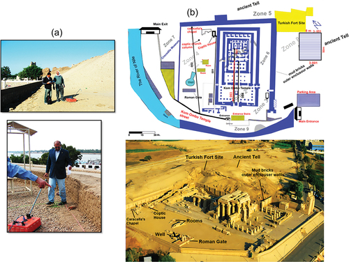
The interest of this study is the Kom Ombo temple (Figure 1), recognised as a significant and unique archaeological site in southern Egypt. Dedicated to the deities Sobek and Horus, the temple is situated approximately forty-eight kilometres north of Aswan city, perched at geographical coordinates (492740 E 2,704,280 N). Constructed during the Greek-Roman period from 332 BC to 395 AD on pre-existing ruins, the temple is believed to encompass cultural layers spanning various historical periods. Geological analysis reveals a landscape characterised by basement and sedimentary rocks, notably the Upper Cretaceous Nubian sandstone group and Quaternary deposits covering extensive areas. Surface silt layers from agricultural activities overlay these geological formations, exhibiting variable thickness along the Nile valley and delta. This study objects to assess the efficacy of FDTD numerical modelling in analysing buried archaeological anomalies within the Kom Ombo temple. According to findings from the dewatering project sponsored by “American Aid” at Kom Ombo temple, Sadarangani et al. (2015), delineated nine distinct zones within the temple premises Figure 2, Zone 1 encompasses the Ptolemaic temple and its outer enclosure walls, Zone 2 positioned west of Zone 1 covering the paved forecourt area, Zone 3 is situated west of the temple, housing the Birth House, Hathor Chapel, and South Gate, Zone 4 is located northwest of the temple, also known as Turkish Court, Zone 5 is positioned between the northeast mud brick enclosure wall and the northeast sandstone wall of the temple, Zone 6 situated southeast, between the outer temple wall and the mud brick enclosure wall, Zone 7 contains various modern structures, including the Crocodile Museum and the Magazine, Zone 8 encompasses the majority of the ancient tell and part of a modern enclosure wall., Zone 9 is located on the western side of the temple. Notably, excavations conducted in 2018 unveiled significant findings, including a sphinx statue from the Ptolemaic period and sandstone pieces attributed to King Ptolemy XII and Cleopatra V, along with mummified crocodiles housed in the Crocodile Museum. These discoveries hint at the possibility of undiscovered tunnels beneath the temple, awaiting further exploration.

Figure 1. Google earth image shows location of the Kom Ombo temple in the south of Egypt.

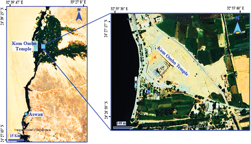
Figure 2. Sketch illustrates (a) GPR survey using GSSI system with 270 MHz central frequency shielded antenna, (b) the distribution of temple’s Zones and GPR survey layout.

2. Materials and methods

2.1. Field acquisition and processing

The SIR 3000 model of the GSSI GPR system, equipped with 270 MHz and 80 MHz antennas, was utilised to gather common offset data at the Kom Ombo temple. These frequencies were chosen to penetrate the temple’s subsurface and reveal its layered structures. In the search for potential subterranean archaeological elements, 55 GPR profiles were recorded, running southwest to northeast, of varying lengths and spacing across Zones (1), (4), and (8) of the temple. Specifically, in Zone (8), a systematic survey was conducted over a (8 m × 50 m) rectangular area consisting of 50 equidistant parallel profiles, as depicted in (Figure 2), with a 1 meter gap between profiles and a 0.1 metre interval between traces. Meanwhile, additional profiles were executed with varying dimensions in Zones (1) and (4).

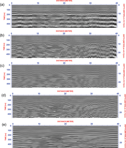
The processing sequence outlined in Figure 3(a–e) was executed using Sandmeier’s (2014) Reflex W 7.5 software, aimed at noise reduction and enhancing recorded data as per Szymczyk’s and Szymczyk (2014) methodology. This included various steps such as scaling correction for time zero adjustment, frequency filtering for band pass frequency, background removal, running average, time gain for energy decay, and velocity analysis on diffraction hyperbolas. Typically, radar waves are diffracted from the top surface of underground structures, necessitating a diffraction stack step to collapse this diffraction and return it to its original location. Interpolation of all 2D processed profiles in Zone (8) was performed to generate time-slices, aiding in illustrating archaeological features more comprehensively in the selected area. Due to variations in length across GPR profiles in Zones (1) and (4) and insufficient data, the geometry of deep anomalies couldn’t be examined through time slices alone. Hence, the Hilbert-Transformation was employed to calculate instantaneous attributes such as the envelope, instantaneous frequency, or phase. These attributes, derived from complex signal theory, were originally applied in the mathematical treatment of amplitude-modulated and frequency-modulated transmission. In this study, the instantaneous amplitude or envelope serves as a measure of reflectivity strength, reflecting the square root of the signal’s total energy at a given instant. The envelope provides an overview of energy distribution within the traces and aids in identifying signal first arrivals (Zhao et al. 2013; Sandmeier 2014).

Figure 3. Processing sequence of GPR data along profile (001) at Zone (a), (a) Raw data of 80 MHz central frequency antenna, (b) time zero adjustment, (c) background removal and frequency filters, (d) energy decay and running average, (e) diffraction stack.

2.2. Numerical modeling

Maxwell’s equations, which mathematically define electromagnetic phenomena, alongside constitutive relationships that quantify material characteristics, form the fundamental framework for quantitatively elucidating GPR signals (Annan 2003). In the frequency domain, Maxwell’s curl equations are pivotal in GPR modelling and the derivation of FDTD equations, as the developed FDTD updating equations can satisfy the divergence equations. The development of GPR modelling codes (Irving and Knight 2006) relies on Maxwell’s curl equations in the frequency domain, which serve as essential elements in this computational approach.

$\mathrm{\nabla }\times \vec{E}=-\mathrm{i}\mathit{\omega }\overrightarrow{\mathit{\mu }\mathrm{H}}(1)\mathrm{Faraday}{}^{\prime }\mathrm{slaw}$

$\mathrm{\nabla }\times \vec{H}=\mathit{\delta }\vec{E}+\mathit{i\omega \epsilon }\vec{E}(2){\mathrm{Ampere}}^{\prime }\mathrm{slaw}$

Using MKS units, where $\stackrel{⃗}{}\mathrm{E}$the electric field intensity (V/m) is, $\overrightarrow{\mathrm{H}}$is the magnetic field intensity (A/m), $\mathit{\sigma }$ is the electric charge density (C/m³). ${\mathit{\epsilon }}_{\mathrm{o}}\mathit{\hspace{0.17em}}$is the free-space permittivity (8.854 × 1012 F/m), ${\mathit{\epsilon }}_{\mathrm{r}}\mathit{\hspace{0.17em}}$is the relative permittivity, and ε=${\mathit{\epsilon }}_{\mathrm{o}}{\mathit{\epsilon }}_{\mathrm{r}}$ is the permittivity (F/m) of the media. Similarly, μo is the free-space permeability (4π×107 H/m), μr is the relative permeability, and μ = μo μr is the permeability (H/m) of the media, $\mathrm{i}=\sqrt{-1\mathit{\hspace{0.17em}}}\mathrm{and}\mathit{\omega }$ is angular frequency. To reduce computation time of solving modified Maxwell’s equations by employing stretching coordinates, the total situation involving a complicated stretched coordinate space is investigated in order to add CPML absorbing barriers into these codes. Where the $\mathrm{\nabla }$ operator takes the following form

(3) $\mathrm{\nabla }=\hat{x}\frac{1}{{\mathrm{s}}_{\mathrm{x}}}\frac{\mathrm{\partial }}{\mathrm{\partial }\mathrm{x}}+\hat{y}\frac{1}{{\mathrm{s}}_{\mathrm{y}}}\frac{\mathrm{\partial }}{\mathrm{\partial }\mathrm{y}}+\hat{z}\frac{1}{{\mathrm{s}}_{\mathrm{z}}}\frac{\mathrm{\partial }}{\mathrm{\partial }\mathrm{z}}$(3)

Where

(4) ${\mathrm{s}}_{\mathrm{k}}={\mathrm{k}}_{\mathrm{k}}+\frac{{\mathit{\sigma }}_{\mathrm{k}}}{{\mathit{\alpha }}_{\mathrm{k}}+\mathrm{i}\mathit{\omega }{\mathit{\epsilon }}_{\mathrm{o}}},\mathrm{k}=\mathrm{x},\mathrm{y},\mathrm{z}$(4)

are complex coordinate stretching variables that vary only in the k direction (Kuzuoglu and Mittra 1996). ${\mathit{\sigma }}_{\mathrm{k}}$, ${\mathrm{k}}_{\mathrm{k}}$, and ${\mathit{\alpha }}_{\mathrm{k}}$ are parameters that can be specified to allow for wave propagation in the interior of the modelling grid and wave absorption in the PML boundary regions. No variation in y direction was assumed and by using transverse magnetic mode (TM-mode) in our modelling the equations (1) and (2) converts to:

(5a) $\mathit{i\omega \mu }{\mathit{H}}_{\mathit{x}}=-\frac{1}{{\mathit{S}}_{\mathit{z}}}\frac{\mathrm{\partial }{\mathit{E}}_{\mathrm{y}}}{\mathrm{\partial }\mathit{z}}\mathit{\hspace{0.17em}}$(5a)

(5b) $\mathit{i\omega \mu }{\mathit{H}}_{\mathit{z}}=\frac{1}{{\mathit{S}}_{\mathit{x}}}\frac{\mathrm{\partial }{\mathit{E}}_{\mathit{y}}}{\mathrm{\partial }\mathit{x}}\mathit{\hspace{0.17em}}$(5b)

(5c) $\mathit{\sigma }{\mathit{E}}_{\mathit{y}}+\mathit{i\omega \epsilon }{\mathit{E}}_{\mathit{y}}=\frac{1}{{\mathit{S}}_{\mathit{x}}}\frac{\mathrm{\partial }{\mathit{H}}_{\mathit{z}}}{\mathrm{\partial }\mathrm{x}}-\frac{1}{{\mathit{S}}_{\mathit{z}}}\frac{\mathrm{\partial }{\mathit{H}}_{\mathit{x}}}{\mathrm{\partial }\mathit{z}}\mathit{\hspace{0.17em}}$(5c)

The Finite Difference Time Domain (FDTD) technique is applied to solve Maxwell’s equations over time using the Yee scheme, which discretizes the electromagnetic geometry problem into spatial grids for electric and magnetic field components. These spatial derivatives are approximated using finite differences, followed by the construction of a set of FDTD updating equations to compute future time steps from past ones. The temporal evolution of these fields characterises the propagation of electromagnetic waves within the simulated medium (Yee 1966; Irving and Knight 2006; Elsherbeni and Demir 2009). To simulate and validate unknown archaeological features detected at the Kom Ombo temple, various synthetic models are generated using Irving and Knight’s MATLAB-based code for two-dimensional surface reflection and boreholes GPR. This code was chosen due to its simplicity, suitability for the study’s objectives, and its capability to accommodate higher orders of the FDTD scheme compared to other programmes like gprMax or MatGPR. For instance, the simulations in this study utilise the FDTD scheme O (2, 4), whereas other programmes are restricted to FDTD scheme O (2, 2). The O (2, 4) scheme employs finite difference expressions with fourth-order accuracy for spatial derivatives and second-order expressions for time derivatives. Additionally, the code incorporates a complex frequency-shifted (convolution) perfectly matched layer (CFS-PML) as an absorbing boundary to prevent reflections from domain edges. The code includes equations governing transverse-magnetic (TM) mode and transverse-electric (TE) mode, with the TM-mode updating FDTD equations being utilised in this study. Consequently, two sets of decoupled partial differential equations are employed, encompassing field components such as $\mathit{\hspace{0.17em}}{\mathrm{H}}_{\mathrm{x}},\mathit{\hspace{0.17em}}{\mathrm{H}}_{\mathrm{z}}$ and$\mathit{\hspace{0.17em}}{\mathrm{E}}_{\mathrm{y}}$ with all TM-mode equations discussed in detail by Irving and Knight (2006).

3. Results and discussion

3.1. GPR data

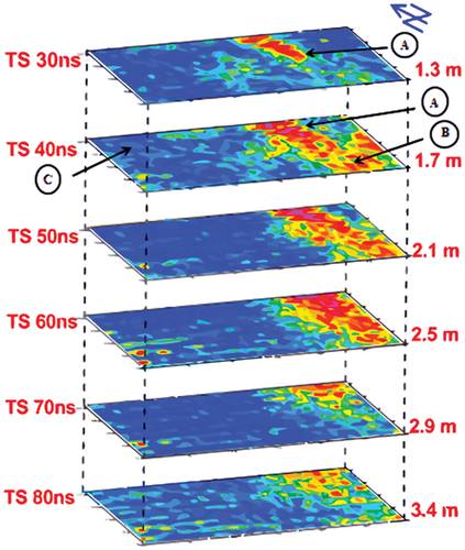
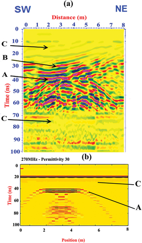
In various zones within the study area, the 2D processed GPR data reveals two notable anomalies. One appears at a shallow depth and corresponds to the 270 MHz central frequency antenna, while the other anomaly is located at a deeper depth and corresponds to the 80 MHz antenna. These anomalies likely pertain to distinct historical periods. Illustrated in Figures 4(a–d), four un-migrated GPR sections near the northeastern part of the temple, known as the “Turkish fort” (Zone 8), depict an anomaly characterised by small overlapping hyperbolas (A) extending into stratigraphic layers (B) at a shallow depth. This anomaly is observed at the outset of the GPR sections, situated in close proximity to the remnants of an ancient fort, warranting further investigation into its nature. Combined time slices of the entire GPR dataset indicate that the mentioned anomalies (A) might hold archaeological significance, as depicted in Figure (5). These time slices suggest the potential presence of an elongated structure, approximately 0.6 metres wide, extending over 15 ns, with its width and amplitude increasing over time before tapering off around 3.8 metres by 90 ns. Recent archaeological studies by Sadarangani et al. (2015) and Forstner et al. (2020) have identified archaeological remnants of ancient walls (A) that correlate with an extension of the Anglo-Egyptian fort known as the “Turkish fort”.

Figure 4. Parallel GPR sections of NE part of Kom Ombo temple represent some reflection events such as (A) hyperbola of extension of Turkish fort mud bricks walls, (B) stratigraphic strata and (C) host medium of silty sand.

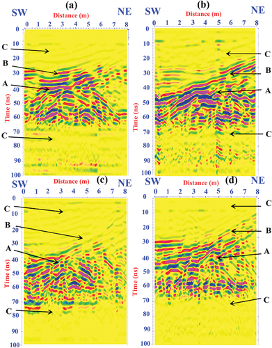
Figure 5. Time slices illustrate the geometry of Turkish fort mud bricks walls, (B) stratigraphic strata and (C) host medium of silty sand.

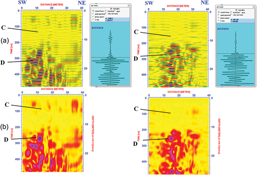
The deep anomaly (illustrated in Figure 6(a,b)) is evident in the GPR data from both Zone (1) within the temple and Zone (4) on its western side, exhibiting the characteristic shape of a large asymmetrical hyperbola (D). To refine the quantitative interpretation of this anomaly, we applied 2D GPR attribute calculations, specifically the envelope, aiming to enhance its clarity. Consequently, we computed the energy distribution (instantaneous amplitude) of all traces within the migrated volume of GPR profiles (001, 002) in Zone (4). The outcome revealed a coherent anomaly in the imaged envelope attribute, situated approximately 11 metres horizontally and 12 metres deep (as depicted in Figure 7(a,b)), corresponding to the deep anomaly. Considering the average electromagnetic velocity (0.11 m/ns), this anomaly is likely associated with reflective rock layers within the limestone structure, embedded within conductive materials such as Silty-Sand (C) (Davis and Annan 1989; Loke 2015). It could represent either a buried archaeological tunnel predating the “Per Sobek” temple or a geological formation. Archaeological findings (cited from Abdel Latif 1970; Beky 1998; Sadarangani et al. 2015) indicate that these types of remains can be found at depths up to 18 metres beneath the current surface. However, justifying this interpretation isn’t feasible because it would be unreasonable to damage the invaluable existing temple to investigate the nature of the anomaly situated 18 metres down. Therefore, numerical modelling techniques are employed to validate the GPR data results and demonstrate their effectiveness in resolving underground ambiguities.

Figure 6. (a, b) Processed GPR sections illustrate deep anomaly (D) and host medium of silty sand (C) inside the temple and on its western side.

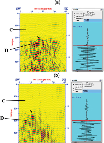
Figure 7. (a) migrated GPR profiles (001, 002) at Zone (4) show anomaly (D) at distance 11 m, depth about 12 m (b) its envelope attribute shows coherent anomaly at distance 11 m and depth about 12 m.

3.2. Numerical models

3.2.1. Shallow anomaly models

Two simulation scenarios are devised to explore the shallow anomaly, each with distinct geometries but identical electrical properties. These synthetic models depict the anomalies as a rectangular body and a stepped-shaped object, as illustrated in Figures (8) and (9). The dimensions of these synthetic models are set at 8 m × 7 m, consisting of two layers: an upper layer of air with ε = 1 and σ = 0, and a lower layer of silty sand with ε = 30 and σ = 0.005 mS/m (Davis and Annan 1989; Loke 2015). The embedded objects are simulated as mud-bricks with ε = 5 and σ = 0.0001 mS/m. All materials are assumed to be non-magnetic (μ = 1). The electromagnetic properties of the various media are detailed in Table 1. The time interval and spatial discretisation values are fixed at dt = 0.014 ns and Δx = Δz = 0.007 m. A GPR transmitter with a centre frequency of 270 MHz is utilised in these simulations.

Figure 8. Synthetic model of rectangular geometry.

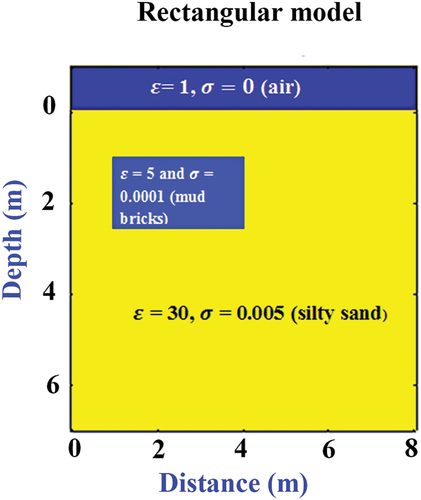
Figure 9. Synthetic model of stepped shape.

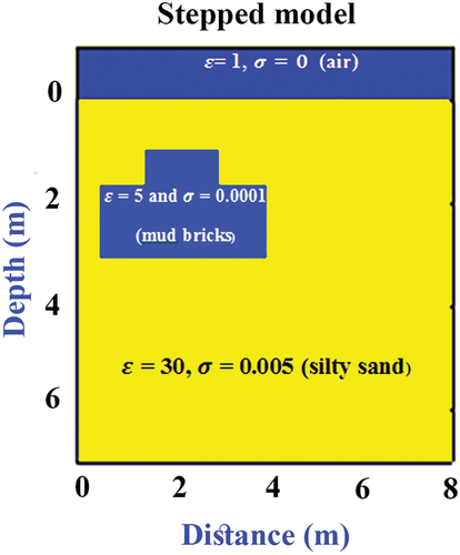
Table 1. Electrical properties of different materials (Davis and Annan 1989; Loke 2015).

No.	Medium	Relative permittivity ε	Electrical conductivity σ (mS/m)	Electromagnetic velocity (m/ns)
1	Air	1	0	0.3
2	Dry sand	3–6	0.1–0.001	0.13–0.17
3	Silty sand	5–30	0.005	0.075
4	Limestone	7–8	0.002–0.00001	0.11
5	Mud bricks	8–40	0.01–1	0.05–0.13

As depicted in Figure (10), significant numerical dispersion is evident post-simulation. This dispersion likely arises from the influence of subsoil permittivity on the wavelength of the propagating wave, leading to its reduction. Thus, to ensure adequate accuracy, it is advisable to finer FDTD cell size, such as (dx/2, dz/2). Through multiple simulation attempts, a high-resolution, low-dispersion image of the reflection from a simulated rectangular model resembling a broad hyperbolic curve (A) was successfully generated, as illustrated in Figure (11). In contrast, the result for the stepped model consists of two distinct elongated hyperbolas (A), as depicted in Figure (12). A comparison between the GPR data results (Figure 13a) and the simulated data (Figure 13b) clearly indicates a correspondence between the shallow anomaly (A) in the GPR data and the broad hyperbolic curve (A) in the simulated rectangular model. They exhibit similar approximate depths and hyperbolic shapes, thus confirming the interpretation of the extension of the walls of the Turkish forts. These walls, characterised by rectangular geometry (A), are constructed from mud-bricks with electrical permittivity values of ε = 5 and conductivity σ = 0.0001 mS/m. Additionally, they are embedded within a silty sand medium (C) with ε = 30 and conductivity σ = 0.005 mS/m.

Figure 10. B-scan of rectangular model with high dispersion.

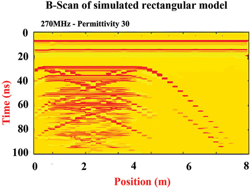
Figure 11. B-scan of low dispersion – simulated rectangular models.

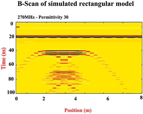
Figure 12. B-Scan of low dispersion- simulated stepped model.

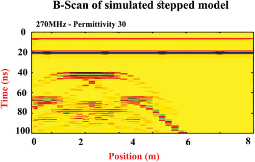
Figure 13. Comparison between (a) GPR section of shallow anomaly and (b) B-scan of low dispersion -simulated rectangular model.

3.2.2. Deep anomaly models

Based on the analysis of a deep anomaly, two scenarios are developed to examine the concealed remains beneath the temple (tunnel or geological formation). The electrical and magnetic properties of all models are identical, despite differing in the suggested geometry of a deep anomaly. These are represented by a symmetric hyperbola and an asymmetric hyperbola. The synthetic models (Figure 14) have dimensions of 40 × 24 metres. These computational domains encompass the surface layer as air with ε = 1 and σ = 0. The second layer is composed of silty sand with ε = 17 and σ = 0.005 mS/m (Davis and Annan 1989; Loke 2015). Subsequently, the physical parameters of the embedded pyramidal, symmetric hyperbola, or asymmetrical hyperbola object are considered for limestone with ε = 8 and σ = 0.0009 mS/m. All materials are assumed to be non-magnetic, such as μ = 1. The time step and spatial increment are determined as dt = 0.04 ns and Δx = Δz = 0.024 m. A Ricker wavelet of a central frequency 80 MHz is used as the source of the GPR transmitter’s signal. The depicted results of simulated models of symmetric hyperbola and asymmetric hyperbola are presented in Figures (15a,b).

Figure 14. Computational domains of (a) symmetric hyperbola and (b) asymmetric hyperbola models.

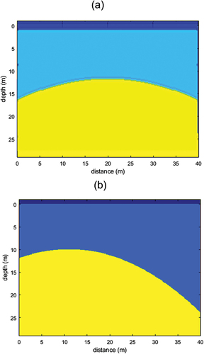
Figure 15. B-scan of the (a) symmetric hyperbola and (b) asymmetric hyperbola models.

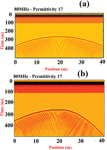
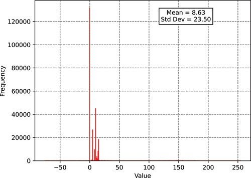
The comparison of all simulated scenarios (Figure 16) suggests that the asymmetric hyperbola (D) model aligns well with the GPR data from the deep anomaly (D) indicating buried artefacts beneath the temple, possibly a tunnel or geological formation. The resemblance between the GPR data and simulated data in terms of shape, features, depths, and distances is depicted and analysed in the histogram (Figure 17), which displays a symmetrical distribution with a peak around 8.63. This leads to the conclusion that the structure under inspection conforms to an asymmetric hyperbola (D), implying the presence of an asymmetrically distributed interface beneath the Kom Ombo temple.

Figure 16. (b) The simulating asymmetric hyperbola model (D) validates (a) deep anomaly (D) under the temple.

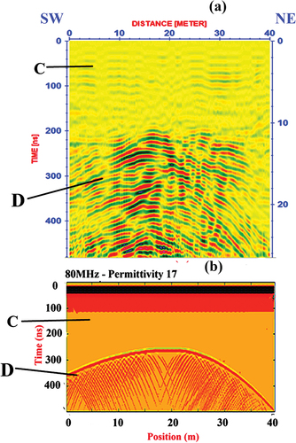
Figure 17. A. symmetrical histogram with a peak near 8.63.

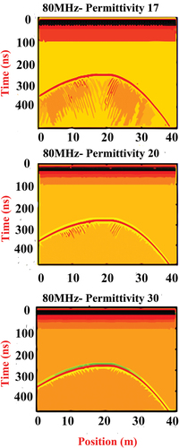
Subsequently, the next target involves determining the physical properties of this structure. Two additional simulations are conducted based on the assumption of an asymmetric hyperbola, maintaining the same dimensions for the synthetic model but varying the electrical properties. Permittivity values of ε = 20 and ε = 30 are chosen to represent different properties of the same lithology, along with ε = 7 to indicate a buried object. These simulations employ a smaller cell size. The results (Figure 18) demonstrate that the synthetic model with ε = 30 offers higher resolution compared to models with lower permittivity values, aligning well with the measured GPR data. This confirms that the buried structure beneath the Kom Ombo temple is likely an archaeological tunnel, characterised by an asymmetrical dome geometry (D), potentially comprising dry limestone rocks with ε = 7 and σ = 0.0009 mS/m, embedded within a silty sand medium (C) with ε = 30 and σ = 0.005 mS/m.

Figure 18. B-Scan from the simulated asymmetric hyperbola model for different values of relative permittivity of silty sand soil.

4. Conclusions and recommendations

4.1. Conclusions

Testing Irving’s and Knight’s code on archaeological case studies, varying in complexity, frequency, and domain size, yielded mostly compatible results with GPR data. The synthetic rectangular model, simulating subsurface properties of a shallow anomaly at 270 MHz central frequency northeast of the temple, suggests an extension of mud-brick walls from a Turkish fort. Similarly, the asymmetric hyperbola model at 80 MHz depicts a deep anomaly inside and west of the temple, possibly remnants of possibly a tunnel or geological formation beneath the current temple. These findings hint at undiscovered historical treasures in the Kom Ombo temple area. Employing FDTD numerical modelling for GPR aids in assessing subsurface properties, determining optimal frequencies, and validating results, offering an enhanced mapping tool for uncovering archaeological features where traditional excavation is impractical.

4.2. Recommendations

1. Utilise numerical modelling to document subsurface findings and validate physical characteristics of archaeological structures like temples, where excavation is challenging.

2. Prioritise numerical approaches before conducting GPR surveys, particularly in heritage areas or archaeological sites, to align work plans and anticipate outcomes, enabling better preparation and strategy adaptation.

3. Future work should focus on enhancing simulation accuracy and resolution, especially for large-scale problems, by employing FDTD scheme O (2, 6) in numerical modelling.

Disclosure statement

No potential conflict of interest was reported by the author(s).

References

- Abbas MA, Salah H, Massoud U, Fouad M, Abdel-Hafez M. 2015. GPR scan assessment at Mekaad Radwan Ottoman – Cairo, Egypt. NRIAG J Astron Geophys. 4(1):106–116. doi: 10.1016/j.nrjag.2015.05.002.
- Abdel Latif M. 1970. Kom Ombo. General Egyptian authority for authoring and publishing. 22–24. In Arabic language.
- Akinsunmade A, Karczewski J, Mazurkiewicz E, TomeckaSuchoń S. 2019. Finite difference time domain (FDTD) modeling of ground penetrating radar pulse energy for locating burial sites. Acta Geophys. 67(6):1945–1953. doi: 10.1007/s11600-019-00352-9.
- Annan AP. 2003. Ground penetrating radar principles, procedures and applications. Sens & Softw Inc. 1–159.
- Beky G. 1998. Egyptian antiquities in Nile valley - Part 4 (from Tiba to Aswan). trans. Alzzirari. 122–126. In Arabic language.
- Bhogapurapu NR, Pandey DK, Venkata Reddy K, Putrevu D. 2019. Study of subsurface roughness impact on GPR performance using modeling and simulation. 10.1007/978-981-13-7067-0_36.
- Davis JL, Annan AP. 1989. Ground-penetrating radar for HIGH-resolution mapping of soil and rock stratigraphy 1. Geophys Prospect. 37(5):531–551. doi: 10.1111/j.1365-2478.1989.tb02221.x.
- Debroux RS. 1996. 3D modelling of the electromagnetic response of geophysical targets using the FDTD method 1. Geophys Prospect. 44(3):457–468. doi: 10.1111/j.1365-2478.1996.tb00157.x.
- Ebrahim Shereen M, Medhat NI, Mansour Khamis K, Gaber A. 2018. Examination of soil effect upon GPR detectability of landmine with different orientations. NRIAG J Astron Geophys. 7(1):90–98. doi: 10.1016/j.nrjag.2017.12.004.
- Elsherbeni ZA, Demir V. 2009. The finite-difference time-domain method for electromagnetics with MATLAB simulations. SciTech Publishing, Inc.; p. 28–453.
- Forstner I, Said A, Rose P, Hassler A, Herbich T, Matic U, Muller S, Ryndziewiez R, Helmbold-Doye J, Palme B, et al. 2020. First report on the Town of Kom Ombo. Osterreichisches archaologisches institute (OAW). Verlag Holzhausen GmbH. 58–92.
- Gamal M, Di Q, Zhang J, Fu C, Ebrahim SM, El-Raouf Amr A. 2023. Utilizing ground-penetrating radar for water leak detection and pipe material characterization in environmental studies: a case study. Remote Sensing. 15(20):4924. doi: 10.3390/rs15204924.
- Holliger K, Bergmann T. 1998. Accurate and efficient FDTD modeling of ground-penetrating radar antenna radiation geophys. Res Lett. 25(20):3883–3886. doi: 10.1029/1998GL900049.
- Irving J, Knight R. 2006. Numerical modeling of ground-penetrating radar in 2-D using MATLAB. Comput Geosci. 32(9):1247–1258. doi: 10.1016/j.cageo.2005.11.006.
- Kuzuoglu M, Mittra R. 1996. Frequency dependence of the constitutive parameters of causal perfectly matched anisotropic absorbers. IEEE Microw Guided Wave Lett. 6(12):447–449. doi: 10.1109/75.544545.
- Liu B, Zhang F, Li S, Sh X, Zhang L, Nie C, Zhang Q. 2018. Forward modeling and imaging of ground-penetrating radar in tunnel ahead geological prospecting. Geophys Prospect. 66(4):784–797. doi: 10.1111/1365-2478.12613.
- Liu SX. 2004. Multi-frequency electromagnetic well logging simulation by 2-D cylindrical FDTD J. Jilin Univ: Earth Sci Ed. 34:283–286. (in Chinese).
- Liu SX, Sato M. 2003. Simulation of borehole radar J. Jilin Univ: Earth Sci Ed. 33:545–550. (in Chinese).
- Liu SX, Sato M. 2005. Transient radiation from an unloaded, finite dipole antenna in a borehole: experimental and numerical results Geophysics 70. GEOPHYSICS. 70(6):k43–k51. doi: 10.1190/1.2106048.
- Loke MH. 2015. Tutorial: 2D and 3D electrical imaging surveys. 4–31.
- Reynolds MJ. 2011. An introduction to applied and environmental geophysics. 2nd ed. pp. 535–537. Chichester. (UK): John Wiley & Sons. Ltd.
- Sadarangani F, Rekaby H, el Khateeb MA. 2015. Desk based assessment for the temple site of Kom Ombo, Aswan Governorate. (Annex to Final Report). 11–161.
- Sandmeier KJ. 2014. ReflexW 7.5 program for the processing of seismic, acoustic or electromagnetic reflection, refraction and transmission data. Zipser Straße1. D-76227 Karlsruhe. Germany.
- Szymczyk M, Szymczyk P. 2014. Processing of GPR data. Image Process & Commun. 18(2–3):83–90. doi: 10.2478/v10248-012-0082-3.
- Teixeira FL, Cho Chew W, Straka M, Oristaglio ML, Wang T. 1998. Finite-difference time-domain simulation of ground penetrating radar on dispersive, inhomogeneous, and conductive soils. IEEE Trans Geosci Remote Sens. 36(6):1928–1937. doi: 10.1109/36.729364.
- Yee KS. 1966. Numerical solution of initial boundary value problems involving Maxwell’s equations in isotropic media. IEEE T Antenn Propag. 14(3):302–307. doi: 10.1109/TAP.1966.1138693.
- Zhao W, Forte E, Pipan M, Tian G. 2013. Ground penetrating radar(GPR) attribute analysis for archaeological prospection. J Appl Geophys. 97:107–117. doi: 10.1016/j.jappgeo.2013.04.010.