Estimating leaf mercury content in Phragmites australis based on leaf hyperspectral reflectance

ABSTRACT

Introduction: High mercury (Hg) concentrations affect the chlorophyll in leaves, thereby modifying leaf spectra. Hyperspectra is a promising technique for the rapid, nondestructive evaluation of leaf Hg content. In this study, we investigated Hg contents and reflective hyperspectra of reed leaves (Phragmites communis) in a gold mining (Jilin province, China). Spectral parameters sensitive to Hg content were identified through basic spectral transformations, continuous wavelet transformation (CWT), and spectral indices techniques. Leaf Hg inversion models were developed using stepwise multiple linear regression, partial least squares regression, and random forest algorithms.Outcomes: The results indicated that: 1) leaf Hg content decreased with increasing distance from the mine: Jiapigou (JPG) > Erdaocha (EDC) > Laojingchang (LJC) > Erdaogou (EDG) > Lingqian (LQ) > Weishahe (WSH). 2) Hg–sensitive wavelengths were primarily in the visible region; CWT increased the correlation between hyperspectral data and leaf Hg content, and improved the regression and accuracy of inversion; 3) the continuum removal–CWT–stepwise multiple linear regression was better for estimating low leaf Hg content; while the differential spectral index–partial least squares regression was better for estimating high leaf Hg content.Conclusion: These hyperspectral inversion methods could be used for rapid, nondestructive monitoring of wetland plants.

KEYWORDS:

• Mercury pollution
• reed leaf
• hyperspectrum
• inversion model
• nondestructive monitoring

Introduction

Mercury (Hg) is a persistent pollutant that is highly toxic and volatile, and readily accumulates in organisms (Angot et al. 2018). It is easily absorbed by plants and undergoes biomagnification that usually occurs in aquatic systems along the food chain, eventually posing a risk to humans (Zhang et al. 2018). Globally, fossil fuel combustion, waste incineration, and mineral processing have elevated the atmospheric Hg concentration 5–fold compared with the level before the industrial revolution (Dunagan, Gilmore, and Varekamp 2007; Selin 2018). It was estimated that Asia contributed 49% of the global atmospheric Hg, and China emitted 583 t Hg and accounted for 26% of the total global emission (Zhang et al. 2015; UNEP, 2019). Therefore, it is critical to monitor environmental Hg contamination in these regions.

Wetlands are an active reservoir of Hg as their abundant water and organic matter provides an environment for Hg accumulation due to atmospheric deposition and runoff (Bachand et al. 2014). Hg can be absorbed by plants and then enters the biosphere (Herndon and Whiteside 2017). Due to the persistent impact and toxicity of Hg and its ability to enter the food chain, Hg accumulation in plants can be further amplified (Liu et al. 2010). Consequently, Hg contamination has become a global public health concern (Herndon and Whiteside 2017). Given the environmental and health impacts of Hg and the roles of plants in the biogeochemical and ecological cycling of this element (Liu et al. 2010), it is critical to monitor Hg levels in plants (Sysalová et al. 2017). Traditionally, monitoring of heavy metals in plants has been conducted by field sampling and laboratory analyses. This method is time–consuming and costly for intensive plant sampling (Liu et al. 2010), and inconvenient for large–scale monitoring (Li et al. 2018). Therefore, it is necessary to develop techniques for rapid monitoring of plant Hg contamination.

Hyperspectroscopy is a technique that is suitable for fast, cost–effective, nondestructive, and large–scale monitoring of plant contamination (Dunagan, Gilmore, and Varekamp 2007; Wang, Gao, and Zha 2018). Integrating spectral and imaging information, this technique can also be used to evaluate the anisotropic distribution of spectral characteristics of plant leaves (Li and Zhang 2018). In previous studies on the use of hyperspectra to estimate plant Hg, screening analyses revealed specific reflectance data that were strongly correlated with the severity of Hg contamination (Dunagan, Gilmore, and Varekamp 2007; Xu 2009; Qiao et al. 2018). For example, Dunagan, Gilmore, and Varekamp (2007) reported that Spinacia oleracea grown in Hg–contaminated soils modified the leaf spectra, with spectral features at bands of 430, 448, 471, and 550 nm, which correlated with the leaf Hg concentration. Xu (2009) found that Zea mays farmed in Hg–contaminated soils had decreased reflectance in the range of 690–740 nm. However, these studies were predominantly focused on agricultural plants such as vegetables and other commercial crops. Few studies have investigated the hyperspectral inversion of Hg concentration in wetland plants, which have important ecological value in production, regulating climate change, purifying water, and providing an ecosystem for many other organisms. It has not been determined whether hyperspectral inversion is a suitable technique for monitoring Hg contamination in wild wetland plants.

In this study, we investigated leaf Hg content in wild reed (Phragmites communis) and its relationship with hyperspectral features. Multiple techniques (spectral transformations, continuous wavelet transformation [CWT], and spectral indices) were used to identify Hg–sensitive parameters from the spectra. Models for the hyperspectral inversion of leaf Hg concentration were then developed with stepwise multiple regression (SMR), partial least squares regression (PLSR), and random forest (RF) algorithms. Our aim was to develop a model for accurate hyperspectral inversion of leaf Hg content in wild reeds that will support the fast, nondestructive, and large–scale monitoring of Hg contamination in wetland plants.

Materials and methods

Study area

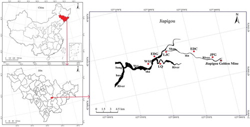
The study was conducted at the Jiapigou gold mine (127°16ʹ–127°39ʹ E, 42°52ʹ–42°56ʹ N; southeast Huadian, Jilin province, China) (Figure 1), located in the upper reach of the Songhua River. The mine is located in a region that hosts >30 gold mining plants. Since 1949, the region has maintained a gold production rate of >1 ton per year (Zhang, Wang, and Wang et al. 2012). Currently, the Jiapigou gold mine is the largest mining plant in the region, and excavates ~2000 tons of ore annually. It started gold extraction using the amalgamation process in 1821 (Yang, Wang, and Cai 2014). Before 2008, the process used ~20 kg Hg per year, and 50%–60% leached into the local soil, water, or atmosphere via point and non–point sources (Wang and Zhu 2000; Wang, Zhu, and Sheng et al. 2005). Between 2006 and 2008, the mine replaced the amalgamation process with a new all–slime cyanidation process (Li, Wang, and Wang 2013); however, the decades of Hg emission have resulted in severe pollution, with soil Hg concentrations reaching 2.2 mg·kg⁻¹ (Zhang et al. 2018), much higher than the standard natural background soil Hg concentration of 0.15 mg·kg⁻¹.

Six sampling sites were selected near the mine along the Shanma River (a tributary of the Songhua River) (Figure 1): Jiapigou (JPG), Erdaocha (EDC), Laojingchang (LJC), Erdaogou (EDG), Weishahe (WSH), and Lingqian (LQ) (listed from up–to downstream). Of these, LQ is an uncontaminated site without mining operations; JPG is a mine with active mining; EDC is a large tailing pond; and LJC and EDG are confluences of rivers. At LJC, the Shanma River joins an uncontaminated river from Wudaogou (an un–mined area without Hg contamination). At EDG, the Weisha River merges with an uncontaminated river from LQ.

Figure 1. Distribution of sampling points

Data collection

Between June and September 2016, five sampling points (each 100 × 100 cm), which were covered by dense reeds and were within 5 km of the river, were established at each of the six sampling sites. Hyperspectra were recorded using a FieldSpec 4 spectroradiometer (350–2500 nm; Analytical Spectral Device, Boulder, CO, USA) in the field at each sampling point. To minimize external interference, intact and undamaged leaves were selected and fully unfolded, then cleaned with water and measured with a leaf clip. Care was taken to avoid the midrib, and whiteboard referencing was conducted every 20 min. The leaves were tested during 10:00–14:00 in bright daylight, with a 5 cm distance between the probe and the middle of the leaf blade to ensure that the leaf occupied the full view of the probe. Three locations were measured on each leaf and the results were averaged. For model development, data from the leaf samples at all sampling points were pooled to ensure sufficient sample sizes. We used the Kennard–Stone (K–S) algorithm to calculate the Euclidean distances in Hg level between all leaf pairs (Yu et al. 2016), and then screened out 41 samples with large differences, which were used for model development (i.e., calibration set). The remaining 27 samples were used for model verification (i.e., validation set) (Table 1). After measurement, the reed leaf samples were transported to the laboratory for analysis, rinsed with water, and dried. The Hg content was measured by cold vapor atomic fluorescence spectroscopy (CVAFS).

Table 1. Summary of leaf mercury (Hg) sample sets

Type of samples	Number	Minimum^# (mg·kg^−1)	Maximum^# (mg·kg^−1)	Mean^# (mg·kg^−1)	Standard deviation (mg·kg^−1)
All samples	68	0.011	0.100	0.035	0.020
Calibration set	41	0.011	0.100	0.036	0.021
Validation set	27	0.020	0.089	0.033	0.017

^#Hg content was measured by cold vapor atomic fluorescence spectroscopy.

Methods

Hyperspectral parameters sensitive to leaf Hg content were identified from spectra by basic spectral transformations, CWT, and spectral indices techniques.

Basic spectral transformations

The basic spectral transformations were first derivative transformations (DR), continuum removal (CR), logarithmic transformation (LR), and normalized transformation (NR) (Equations 1(1) $DR=\frac{{\rho }_{\lambda i+1}-{\rho }_{\lambda i-1}}{2\mathrm{\Delta }\lambda }$(1) –4(4) $NR=\frac{{\rho }_{\lambda i}}{\frac{1}{n}\sum _{i=1}^n{\rho }_{\lambda i}}$(4) ), which effectively improved the contrast of different hyperspectral absorption characteristics. Original hyperspectral reflectance was abbreviated to Ro, Ro processed by DR was abbreviated to DR, and so forth.

(1) $DR=\frac{{\rho }_{\lambda i+1}-{\rho }_{\lambda i-1}}{2\mathrm{\Delta }\lambda }$(1)

(2) $CR=\frac{{\rho }_{\lambda i}}{{\rho }_{850}+\frac{{\rho }_{2500}-{\rho }_{850}}{2500-850}\ast ({\rho }_{\lambda i}-{\rho }_{850})}$(2)

(3) $LR=log\frac{1}{{\rho }_{\lambda i}}$(3)

(4) $NR=\frac{{\rho }_{\lambda i}}{\frac{1}{n}\sum _{i=1}^n{\rho }_{\lambda i}}$(4)

where ρ_λi-1, ρ_λi, and ρ_λi+1 represent the reflectance at wavelengths λ_i-1, λ_i, and λ_i+1, respectively; and Δλ is the wavelength distance between λ_i and λ_i+1.

Continuous wavelet transformation

CWT reveals subtle variations that are difficult to discern from the original spectral data. In addition, CWT decomposes hyperspectral data continuously giving wavelet coefficients that match well with the original spectral data and enable extraction of fine signals from raw data (Liang et al. 2015). In this study, we used CWT to decompose the hyperspectral data into two series of wavelet coefficients under different scales (Equations 5(5) $Wf(a,b)\le f;{\phi }_{a,b}\ge {\int }_{-\mathrm{\infty }}^{+\mathrm{\infty }}f(t){\phi }_{a,b}(t)dt$(5) and 6(6) ${\phi }_{a,b}(t)=\frac{1}{\sqrt{a}}\phi (\frac{t-b}{a})$(6) ) (Cheng et al. 2010).

(5) $Wf(a,b)\le f;{\phi }_{a,b}\ge {\int }_{-\mathrm{\infty }}^{+\mathrm{\infty }}f(t){\phi }_{a,b}(t)dt$(5)

(6) ${\phi }_{a,b}(t)=\frac{1}{\sqrt{a}}\phi (\frac{t-b}{a})$(6)

where f(t) represents hyperspectral reflectance (350–2500 nm) measured from a leaf; t is the wavelength interval (350–25,000 nm); ψ_{a, b}(t) is the basic function; a is the scaling factor; and b is the shift factor.

Coefficients better reveal the characteristic features in hyperspectra (shape and wavelength; Yu et al. 2016). The coefficients comprise two series: i (i = 1, 2, …, m) and j (j = 1, 2, …, n), expressed as an m × n matrix. Series i represents the decomposition scale, and j the bands. By correlating the coefficients with leaf Hg data, the optimum decomposition scale can be determined. In this study, the Mexican hat wavelet that performs well for hyperspectral decomposition (Cheng et al. 2010; Zhang et al. 2014) was used as the basic function, and Ro, DR, CR, LR, and NR were processed by CWT under 10 scales (2¹, 2², 2³ … 2¹⁰).

Spectral indices

Constructing spectral indices involves changing simple Ro data into more complex bands by combining information at multiple bands. This serves various purposes, such as increasing loading information, enlarging the differences between bands (Liu, Gong, and Zhao 2014), maximizing reflective information, and minimizing external interferences (Yang et al. 2009). In this study, the differential spectral index (DSI), ratio spectral index (RSI), and normalized spectral index (NDSI) (Equations 7(7) $DSI={\rho }_{\lambda 1}-{\rho }_{\lambda 2}$(7) –9(9) $NDSI=\frac{{\rho }_{\lambda 1}-{\rho }_{\lambda 2}}{{\rho }_{\lambda 1}+{\rho }_{\lambda 2}}$(9) ), which are the most commonly used, were chosen to establish models for the identification of hyperspectral characteristics of reed leaves and Hg–sensitive wavelengths. To reduce data redundancy, Ro data (350–2500 nm) were resampled (interval: 5 nm) before spectral index calculations, giving 430 bands. Then, DSI, RSI, and NDSI were calculated from all possible combinations of the 430 bands.

(7) $DSI={\rho }_{\lambda 1}-{\rho }_{\lambda 2}$(7)

(8) $RSI=\frac{{\rho }_{\lambda 1}}{{\rho }_{\lambda 2}}$(8)

(9) $NDSI=\frac{{\rho }_{\lambda 1}-{\rho }_{\lambda 2}}{{\rho }_{\lambda 1}+{\rho }_{\lambda 2}}$(9)

where ρ_λi is the reflectance at wavelength λ_i. In these equations, λ₁ ≠ λ₂.

Model development and verification

Stepwise multiple linear regression (SMLR), partial least squares regression (PLSR) and random forest (RF) algorithms, which are the most commonly used in hyperspectral inversion, were employed to develop models for leaf Hg inversion from hyperspectral data. The SMLR method selects the independent variable for the regression equation step–by–step according to the importance of the independent variable. The PLSR method establishes a linear regression model by projecting the predicted variables and the observable variables into a new space. The RF method uses bootstrap resampling and develops decision trees. The predictive power of an inversion model is quantified by its coefficient of determination (R²), and its accuracy is indicated by the root mean square error (RMSE; He 2015). An R² approaching 1 and an RMSE approaching 0 indicate excellent regression. R² > 0.25 and R² > 0.64 were regarded as acceptable and preferable criteria for the calibration and validation sets, respectively (He 2015; Wang 2019).

Results

Reed leaf Hg contents

The average reed leaf Hg content at the six sampling sites is shown in Table 2. The leaf Hg content decreased with increasing distance from JPG. The leaf Hg content was higher at JPG and EDC than at LJC, EDG, WSH, and LQ.

Table 2. Reed leaf mercury (Hg) content at different sampling sites

Sampling sites	Number of samples	Leaf Hg content (mg·kg^−1)
JPG	11	0.133 ± 0.086
EDC	11	0.075 ± 0.055
LJC	10	0.040 ± 0.016
EDG	12	0.034 ± 0.009
WSH	11	0.027 ± 0.007
LQ	13	0.029 ± 0.010
Average		0.056 ± 0.009

JPG–Jiapigou, EDC–Erdaocha, LJC–Laojingchang, EDG–Erdaogou, WSH–Weishahe, and LQ–Lingqian; Values are means ± standard deviation (n = 5).

Identification of Hg–sensitive hyperspectral parameters

Identification based on basic transformations

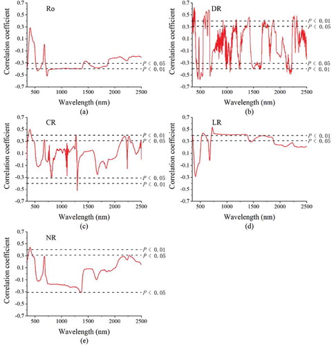
Correlation analyses were performed between leaf Hg content and hyperspectral data (Figure 2). For Ro, significant negative correlations with leaf Hg content were found for the intervals 350–362, 516–647 (visible region), 696–1300 (near–infrared), 1301–1411, and 1507–1872 nm (mid–infrared) (p < 0.05; absolute value of maximum correlation coefficient (R): 0.521, 726 nm; Figure 2a). For DR, the R fluctuated sharply with wavelength and many Hg–sensitive wavelength intervals were scattered within the spectral range; the maximum R was 0.628 (389 nm; Figure 2b). For CR, a few Hg–sensitive intervals were found, including significant positive correlations at 361–464, 673–682 (visible), 1265–1278 (near–infrared), 2126–2216, and 2250–2290 nm (mid–infrared) and a significant negative correlation at 1293–1301 nm (p < 0.05; maximum R: 0.502, 405 nm; Figure 2c). For LR, the R curve resembled an inverted form of Ro, exhibiting similar Hg–sensitive intervals but increased R values (maximum R: 0.536, 726 nm; Figure 2d). For NR, the R curve was somewhat similar to that of Ro, but had lower R values and fewer Hg–sensitive intervals, with a significant positive association at 376–451 nm (visible) and a significant negative association at 1359–1374 nm (mid–infrared) (p < 0.05; maximum R: 0.441, 406 nm; Figure 2e). Therefore, DR and LR transformations improved the correlations between hyperspectral data and leaf Hg content. The Hg–sensitive intervals identified were predominantly in the visible range after data transformation.

Figure 2. Correlation coefficients between leaf mercury (Hg) content and spectral reflectance data before and after different transformations: (a) original spectral reflectance (Ro); (b) first derivative transformation (DR); (c) continuum removal (CR); (d) logarithmic transformation (LR); (e) normalized transformation (NR)

Identification based on continuous wavelet transformation

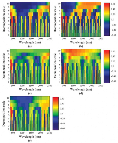
Hyperspectral data were decomposed by CWT and the resulting wavelet coefficients were analyzed for correlations with leaf Hg content. The R values were improved under all decomposition scales after CWT. For Ro–CWT, the maximum R was 0.651; for DR–CWT, it was 0.644; for CR–CWT, 0.662; for LR–CWT, 0.661; and for NR–CWT, 0.661 (Figure 3).

Figure 3. Correlation coefficient diagram between leaf Hg content and wavelet coefficients before and after different continuous wavelet transformations: (a) original spectral reflectance (Ro); (b) first derivative transformation (DR); (c) continuum removal (CR); (d) logarithmic transformation (LR); (e) normalized transformation (NR). (red: strong positive correlation; blue: strong negative association)

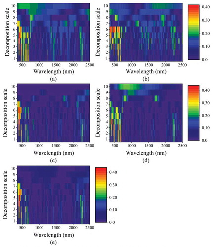
Examination of the R² values revealed that Ro–CWT correlated well with leaf Hg content (R² > 0.25) at seven intervals (350–495, 529–596, 598–628, 637–691, 736–742, 1251–1253, and 1619–1621 nm), reaching local maxima at 401 (decomposition scale 4), 549 (scale 1), 602 (scale 1), 655 (scale 1), 739 (scale 5), 1252 (scale 1), and 1620 nm (scale 2) (Figure 4a). The DR–CWT data correlated well with leaf Hg content at five intervals (351–539, 568–674, 701–712, 1573–1581, and 2380–2387 nm), reaching local maxima at 463 (scale 6), 575 (scale 1), 706 (scale 5), 1579 (scale 4), and 2383 nm (scale 4) (Figure 4b). The CR–CWT data correlated well with leaf Hg content at six intervals (350–489, 598–610, 623–628, 654–659, 680–685, and 2270–2280 nm), reaching local maxima at 403 (scale 4), 601 (scale 3), 626 (scale 3), 657 (scale 2), 683 (scale 5), and 2273 nm (scale 2) (Figure 4c). The LR–CWT data correlated well with leaf Hg content at seven intervals (352–379, 394–443, 460–496, 519–627, 634–684, 782–816, and 2271–2281 nm), reaching local maxima at 362 (scale 2), 405 (scale 1), 465 (scale 3), 572 (scale 1), 656 (scale 1), 800 (scale 8), and 2273 nm (scale 2) (Figure 4d). Finally, NR–CWT correlated well with leaf Hg content at five intervals (371–488, 598–611, 623–628, 654–660, and 2271–2282 nm), with local maxima at 466 (scale 3), 600 (scale 3), 626 (scale 3), 657 (scale 2), and 2273 nm (scale 2) (Figure 4e). Therefore, there were good correlations between transformed spectral data in the visible range and leaf Hg content, and decompositions on small scales generally improved the correlations after CWT.

Figure 4. Coefficients of determination (R²) between leaf Hg content and wavelet coefficients before and after different continuous wavelet transformations: (a) original spectral reflectance (Ro); (b) first derivative transformation (DR); (c) continuum removal (CR); (d) logarithmic transformation (LR); (e) normalized transformation (NR). (red: strong positive correlation; blue: strong negative association)

Identification based on spectral indices

Spectral indices (i.e., DSI, NDSI and RSI) sensitive to leaf Hg content were calculated for all possible band combinations (Figure 5). The three spectral indices showed similar correlations with leaf Hg content. However, the bands with high correlations between DSI and leaf Hg content had significantly higher correlation coefficients than those between leaf Hg content and NDSI or RSI (Figure 5a). These regions were scattered on the equipotential diagram, covering all spectral ranges.

Figure 5. Equipotential diagram illustrating coefficients of correlations between leaf Hg content and (a) differential spectral index (DSI); (b) normalization spectral index (NSI), and (c) ratio spectral index (RSI)

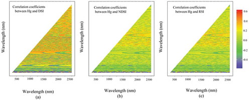
Table 3 summarizes all Hg–sensitive spectral indices with R > 0.6. The Hg–sensitive band combinations included visible/near–infrared, visible/mid–infrared, and visible–visible pairs. The maximum R value was obtained for the 350/520 nm combination.

Table 3. Summary of spectral indices with a correlation coefficient >0.6

Spectral indices	Band 1 (nm)	Band 2 (nm)
DSI	350	520–530
	375	1655
NDSI	350	520–530
	370	1585, 1890–1900, 2205–2210
RSI	350	520–530
	370	1580–1585, 1885–1900, 2200–2215

DSI, differential spectral index; NDSI, normalized spectral index; and RSI, ratio spectral index.

Leaf Hg inversion

Inversion based on spectral transformations

For modeling, leaf Hg content was used as the independent variable; for Ro, DR, CR, LR, and NR, Hg–sensitive bands with statistically significant correlations with leaf Hg content (R > 0.5, p < 0.01) were used as dependent variables; and for Ro–CWT, DR–CWT, CR–CWT, LR–CWT and NR–CWT, Hg–sensitive wavelet coefficients (R > 0.5, p < 0.01) were used as dependent variables. Inversion models were developed by SMLR, PLSR, and RF (Table 4). The SMLR models developed from DR and LR–CWT were overfitted; NR had no wavelength with R > 0.5 (Figure 2e). These data were not used for modeling.

Table 4. Inversion accuracy of calibration set and validation set of models based on spectral transformations

	Calibration set		Validation set
Model	R^2	RMSE	R^2	RMSE
Ro-SMLR	0.2717	0.0179	0.2762	0.0186
Ro-PLSR	0.2720	0.0179	0.2766	0.0186
Ro-RF	0.4114	0.0175	0.4178	0.0218
DR-PLSR	0.6691	0.0121	0.8126	0.0194
DR-RF	0.3445	0.0171	0.5546	0.0187
CR-SMLR	0.3690	0.0167	0.2554	0.0150
CR-PLSR	0.3680	0.0167	0.2534	0.0150
CR-RF	0.2757	0.0174	0.3572	0.0167
LR-SMLR	0.2871	0.0177	0.2812	0.0186
LR-PLSR	0.2872	0.0177	0.2834	0.0186
LR-RF	0.4104	0.0175	0.4139	0.0218
Ro-CWT-SMLR	0.4241	0.0159	0.5373	0.0173
Ro-CWT-PLSR	0.5547	0.0140	0.6104	0.0169
Ro-CWT-RF	0.4660	0.0204	0.7920	0.0191
DR-CWT-SMLR	0.5580	0.0140	0.4069	0.0169
DR-CWT-PLSR	0.5366	0.0143	0.7404	0.0179
DR-CWT-RF	0.4831	0.0162	0.5564	0.0111
CR-CWT-SMLR	0.5619	0.0139	0.8170	0.0173
CR-CWT-PLSR	0.5198	0.0146	0.7185	0.0187
CR-CWT-RF	0.4710	0.0173	0.8609	0.0194
LR-CWT-PLSR	0.5111	0.0147	0.8288	0.0196
LR-CWT-RF	0.4761	0.0140	0.7483	0.0187
NR-CWT-SMLR	0.5487	0.0141	0.7386	0.0178
NR-CWT-PLSR	0.5293	0.0144	0.7833	0.0182
NR-CWT-RF	0.5504	0.0175	0.6008	0.0186

Ro, original spectral reflectance; SMLR, stepwise multiple linear regression; PLSR, partial least squares regression; RF, random forest; DR, first derivative transformation; CR, continuum removal; LR, logarithmic transformation; CWT, continuous wavelet transform; NR, normalized transformation; R², coefficient of determination; RMSE, root mean square error.

Further analyses indicated that the models developed from Ro, DR, CR, and LR generally exhibited unsatisfactory fits. DR–PLSR yielded R² > 0.64 and showed the highest R² allowing leaf Hg inversion. For CWT–processed data, calibration models developed by SMLR and PLSR exhibited acceptable fits, whereas those developed by RF did not. Validation sets developed by PLSR and RF offered better fits than those developed by SMLR. Of all the models developed, eight exhibited better fits for both the calibration and validation sets: CR–CWT–SMLR, NR–CWT–SMLR, Ro–CWT–PLSR, DR–CWT–PLSR, CR–CWT–PLSR, LR–CWT–PLSR, NR–CWT–PLSR, and NR–CWT–RF.

Compared with the models developed from data that did not undergo CWT, those developed using CWT–processed data had improved fits and accuracies in both calibration (R² increased by 0.0386–0.2239; RMSE increased by 0.0001–0.0121) and validation (R² increased by 0.0018–0.5454; RMSE increased by 0.0013–0.0076). Of all the models examined, CR–CWT–SMLR exhibited the high prediction accuracy and the low RMSE (Table 4), indicating that it was the best model for leaf Hg inversion.

Leaf Hg inversion based on spectral indices

Inversion models were developed by SMLR, PLSR, and RF using leaf Hg content as the dependent variable, and spectral indices with R > 0.5 (i.e., DSI, NDSI and RSI) as the independent variable (Table 5). The three spectral indices were ranked on the basis of their regressions as follows: SMLR > PLSR > RF. Of the models shown in Table 5, only DSI–SMLR and DSI–PLSR showed a high R² on both the calibration and validation sets. Unlike the DSI–SMLR algorithm, the DSI–PLSR algorithm can overcome multicollinearity. Therefore, it was selected for subsequent leaf Hg inversion.

Table 5. Inversion accuracy of the calibration set and validation set of inversion models based on spectral indices

Model	Calibration set		Validation set
	R^2	RMSE	R^2	RMSE
DSI–SMLR	0.5375	0.0143	0.5822	0.0177
DSI–PLSR	0.5290	0.0144	0.5712	0.0176
DSI–RF	0.3849	0.0175	0.5398	0.0179
NDSI–SMLR	0.4449	0.0156	0.6843	0.0185
NDSI–PLSR	0.4362	0.0158	0.6486	0.0182
NDSI–RF	0.4190	0.0175	0.5936	0.0171
RSI–SMLR	0.4466	0.0156	0.6840	0.0185
RSI–PLSR	0.4390	0.0157	0.6444	0.0182
RSI–RF	0.4694	0.0176	0.6301	0.0172

DSI, differential spectral index; SMLR, stepwise multiple linear regression; PLSR, partial least squares regression; RF, random forest; NDSI, normalized spectral index; RSI, stepwise multiple linear regression; R², coefficient of determination; RMSE, root mean square error.

Verification of inversion models

The CR–CWT–SMLR and DSI–PLSR models were verified for leaf samples from all sites (Table 6). The CR–CWT–SMLR model performed satisfactorily (R² > 0.8) for all sites except JPG, and the sites were ranked, from highest R² value to lowest, as follows: LQ > WSH > EDG > LJC > EDC. The sites were ranked in almost the opposite order on the basis of R² values for the DSI–PLSR model: JPG > EDC > LJC > WSH > EDG > LQ.

Table 6. Inversion accuracy of models at different sampling sites

Model	Sampling site	R^2	RMSE
CR–CWT–SMLR	JPG	0.7050	0.0614
	EDC	0.8850	0.0057
	LJC	0.8510	0.0093
	EDG	0.8970	0.0040
	WSH	0.9040	0.0026
	LQ	0.9430	0.0014
DSI–PLSR	JPG	0.9889	0.0002
	EDC	0.9539	0.0034
	LJC	0.8454	0.0090
	EDG	0.5133	0.0084
	WSH	0.8501	0.0031
	LQ	0.4919	0.0040

CR–CWT–SMLR, continuum removal–continuous wavelet transform–stepwise multiple linear regression; DSI–PLSR, differential spectral index–partial least squares regression; JPG–Jiapigou, EDC–Erdaocha, LJC–Laojingchang, EDG–Erdaogou, WSH–Weishahe, and LQ–Lingqian; R², coefficient of determination; RMSE, root mean square error.

Discussion

Identification of Hg–sensitive parameters and development of leaf Hg inversion model

High Hg concentration can decrease the chlorophyll content (Kupper, Kupper, and Spiller 1996), destroy the cellular structure, and change the permeability of cell membranes in the plant leaves (Yuan and Ding 2016), thereby causing reflective refractive discontinuity and modifying leaf spectra information, such as the red edge shifting toward the low–band direction, the green peak showing increased reflectance, and the red valley becoming shallower by increasing or decreasing the reflectivity (Maruthi Sridhar et al. 2007; Chi, Guo, and Chen 2017; Li 2018). In this study, the Hg–sensitive wavelengths identified from the data processed by basic spectral transformations and CWT were mainly in the visible region, consistent with the findings of another study on the correlations between hyperspectral reflectance of reed leaves and the heavy metals lead and copper (Zhou 2014). Wavelet coefficient screening and inversion modeling showed that after CWT, the correlation between reflectance and leaf Hg content increased substantially (Figure 3), and the R² and RMSE of prediction also improved (Table 4). Similar results were obtained in our earlier study on hyperspectral Hg inversion of reed leaves grown under controlled Hg exposure (Li et al. 2018). This improvement may be attributable to the characteristics of wavelet transformations that decompose hyperspectral data in both time and frequency domains. It is thus possible to screen optimum signals on different scales to predict physio–biochemical characteristics of plants (Song et al. 2006, 2008; Li et al. 2018). As compared with discrete wavelet transformation, CWT decomposes hyperspectral data continuously giving wavelet coefficients that match well with the original spectral data and enable extraction of fine signals from raw data. Therefore, compared with discrete wavelet transformation, CWT allows for clearer characterization of spectral signals (Fang, Le, and Liang 2015; Liang et al. 2015). In addition, CWT reveals subtle variations that are difficult to discern from the original spectral data, thus allowing the discovery of hidden information and improving the accuracy of inversion compared with analyses that do not include CWT (Yu et al. 2016). Due to these advantages, CWT is an important technique for the hyperspectral determination of Hg content in reed leaves.

In this study, analyses of leaf Hg inversion based on hyperspectral transforms and spectral indices showed that CR–CWT–SMLR and DSI–PLSR performed better than RF. In our earlier study on Hg inversion for reed leaves grown under controlled Hg exposure, an RF model performed better than PLSR and SMR models (Li et al. 2018). This difference may be attributed to the relatively small dataset of the current field study, which failed to fully exploit the advantages of the RF algorithm. Instead, commonly used empirical or semi–empirical modeling (particularly PLSR, which overcomes multicollinearity) algorithms performed better in this study.

Model verification with measured leaf Hg content data from the sampling sites showed that the CR–CWT–SMLR model ranked the sites, from highest R² value to lowest, as follows: LQ > WSH > EDG > LJC > EDC > JPG, whereas the ranking based on the R² values of the DSI–PLSR model showed almost the opposite trend (Table 6). This difference might have resulted from the geographic distribution of the sampling sites. Of all the sites studied, JPG was nearest the gold mine and thus, reeds at this site had the highest leaf Hg content. The other sites were a distance from the mine in ascending order of EDC, LJC, EDG, WSH, and LQ. Accordingly, the reed leaf Hg contents at these sites generally decreased sequentially (Table 2). The R² of leaf Hg content predicted using the CR–CWT–SMLR model decreased with increasing Hg content; therefore, this model was stable and reliable at low leaf Hg content. In comparison, DSI–PLSR was reliable for sites with high leaf Hg content, but was less reliable for predicting low leaf Hg content.

Limitations and implications

Due to the limitations in sampling conditions and workload, we did not consider the effects of other factors, such as, climatic factors, on the performance of spectral indices to estimate the Hg content of reed leaves. Further studies should be carried out to evaluate variations in spectral indices of reed leaves related to differences in moisture, season, and/or other co–existing factors. In addition, the R² of the validation sets of the accepted leaf Hg inversion models were much higher than those in the calibration sets (Tables 4 and 5), and this may be attributed to the small number of sampling sites and small difference between the validation samples. These findings also indicate that the robustness of the models requires verification with more samples. However, in this study, leaf sample data from all the sampling points were used by pooling and filtering. We will conduct supplementary experiments in the future to collect samples for verification of robustness. Finally, further research should focus on technical methods to monitor Hg in reeds and other plants such as grasses and forest species in polluted areas, in order to better verify the method and expand the scope of its application.

Conclusion

Reed leaves were collected from a gold mining region to determine the relationship between leaf Hg content and the characteristics of reflective hyperspectra. Spectral transformation techniques were used to identify Hg–sensitive data. Based on the models developed by SMLR, PLSR, and RF algorithms, we investigated the correlations between the identified data and leaf Hg content, and inversed the leaf Hg content. The main results were as follows:

1. Wavelengths sensitive to leaf Hg content were primarily in the visible region. Hyperspectral data processed by CWT showed stronger correlations with leaf Hg content than the original hyperspectral data. The Hg–sensitive wavelengths identified based on spectral indices showed a strong correlation in the 350/520 nm combination.

2. Inversion models developed based on CWT–processed data improved regression and accuracy both for the calibration and validation sets. Of all the models, the CR–CWT–SMLR model resulted in the best inversion (R²) for estimating low leaf Hg content, while the DSI–PLSR model performed best for estimating high leaf Hg contents.

Disclosure statement

No potential conflict of interest was reported by the authors.

Additional information

Funding

This work was supported by the Fundamental Research Funds of Central-level Nonprofit Research Institutes of China [CAFINT2014K05].

References

- Angot, H., N. Hoffman, A. Giang, C. P. Thackray, A. N. Hendricks, N. R. Urban, and N. E. Selin. 2018. “Global and Local Impacts of Delayed Mercury Mitigation Efforts.” Environmental Science & Technology 52: 12968–11. doi:10.1021/acs.est.8b04542.
- Bachand, P. A. M., S. M. Bachand, J. A. Fleck, C. N. Alpers, M. Stephenson, and L. Windham-Myers. 2014. “Methylmercury Production in and Export from Agricultural Wetlands in California, USA: The Need to Account for Physical Transport Processes into and Out of the Root Zone.” Science of the Total Environment 472: 957–970. doi:10.1016/j.scitotenv.2013.11.086.
- Cheng, T., B. Rivard, G. A. Sánchezazofeifa, J. Feng, M. Calvo-Polanco. 2010. “Continuous Wavelet Analysis for the Detection of Green Attack Damage Due to Mountain Pine Beetle Infestation.” Remote Sensing of Environment 114 (4): 899–910. DOI:10.1016/j.rse.2009.12.005.
- Chi, G. Y., N. Guo, and X. Chen. 2017. “Hyperspectral Remote Sensing Monitoring on Heavy Metal Contaminated Farmland.” Soils Crops 6: 243–250.
- Dunagan, S. C., M. S. Gilmore, and J. C. Varekamp. 2007. “Effects of Mercury on Visible/near-infrared Reflectance Spectra of Mustard Spinach Plants (Brassica Rapa P.).” Environmental Pollution 148: 301–311. doi:10.1016/j.envpol.2006.10.023.
- Fang, S. H., Y. Le, and Q. Liang. 2015. “Retrieval of Chlorophyll Content Using Continuous Wavelet Analysis across a Range of Vegetation Species.” Geomatics and Information Science of Wuhan University 40 (3): 296–302. in Chinese.
- He, J. 2015. “Monitoring Model of Ecological and Physiological Parameters of Winter Wheat Based on Hyperspectral Reflectance at Different Growth Stages.” Doctor Thesis, Northwest A&F University, Yangling. ( in Chinese).
- Herndon, J. M., and M. Whiteside. 2017. “Contamination of the Biosphere with Mercury: Another Potential Consequence of On-going Climate Manipulation Using Aerosolized Coal Fly Ash.” Journal of Geography, Environment and Earth Science International 13 (1): 1–11. JGEESI. 37308. doi:10.9734/JGEESI.
- Kupper, H., F. Kupper, and M. Spiller. 1996. “Environmental Relevance of Heavy Metal~substituted Chlorophylls Using the Example of Water Plants.” Journal of Experimental Botany 47 (295): 259–266. doi:10.1093/jxb/47.2.259.
- Li, J. Y., and Y. C. Zhang. 2018. “Hyperspectral Prediction Model of Cadmium Content in Lettuce Leaves.” Agricultural Engineering 8 (3): 65–69. in Chinese.
- Li, M. 2018. “Hyperspectral Feature and Mercury Content Inversion of Reed Leaves under Mercury Pollution.” Master Thesis, Chinese Academy of Forestry, Beijing. ( in Chinese).
- Li, M. J, M. Y. Zhang, L. J. Cui, H. N. Wang, Z. L. Guo, W. Li, Y. Y. Wei, S. Yang, and S. Y. Long. 2018. “Inversion of Hg Content in Reed Leaves Based on Continuous Wavelet Transform and Random Forest.” Chinese Journal of Eco-Agriculture 26: 1730–1738.
- Li, Y. F., J. Wang, and N. Wang. 2013. “Distribution Characteristics and Risk Assessment of Mercury Pollution in the River Water and Sediment of the Songhua River Upstream Gold Mining Area.” Journal of Agro-Environment Science 32 (3): 622–628. in Chinese.
- Liang, D., Q. Y. Yang, W. J. Huang, D. L. Peng, J. L. Zhao, L. S. Huang, D. Y. Zhang, and X. Y. Song. 2015. “Estimation of Leaf Area Index Based on Wavelet Transforms and Support Vector Machine Regression in Winter Wheat.” Infrared and Laser Engineering 44 (1): 335–340. ( in Chinese).
- Liu, H., Z. N. Gong, and W. J. Zhao. 2014. “Estimating Total Nitrogen Content in Reclaimed Water Based on Hyperspectral Reflectance Information from Emergent Plants: A Case Study of Mencheng Lake Wetland Park in Beijing, China.” Chinese Journal of Applied Ecology 25 (12): 3609–3618. in Chinese.
- Liu, Y., H. Chen, G. Wu, and X. Wu. 2010. “Feasibility of Estimating Heavy Metal Concentrations in Phragmites Australis Using Laboratory-based Hyperspectral data—A Case Study along Le’an River, China.” International Journal of Applied Earth Observation and Geoinformation 12: S166–S170. doi:10.1016/j.jag.2010.01.003.
- Maruthi Sridhar, B. B., F. X. Han, S. V. Diehl, D. L. Monts, and Y. Su. 2007. “Spectral Reflectance and Leaf Internal Structure Changes of Barley Plants Due to Phytoextraction of Zinc and Cadmium.” International Journal of Remote Sensing 28 (5): 1041–1054. doi:10.1080/01431160500075832.
- Qiao, X. Y., S. Y. Ma, H. F. Hou, and R. J. Hao. 2018. “Hyper-spectral Features of Heavy Metal Pollutants in Vegetables and Their Inversion Model in the Mining Areas.” Journal of Safety and Environment 18 (1): 335–341. in Chinese.
- Selin, N. E. 2018. “A Proposed Global Metric to Aid Mercury Pollution Policy.” Science 360: 607–609. doi:10.1126/science.aar8256.
- Song, K. S., B. Zhang, Z. M. Wang, F. Li, and H. J. Liu. 2006. “Application of Wavelet Transformation in In-situ Measured Hyper Spectral Data for Soybean LAI Estimation.” Chinese Agricultural Science Bulletin 22 (9): 101–108. in Chinese.
- Song, K. S., B. Zhang, Z. M. Wang, D. W. Liu, and H. J. Liu. 2008. “Soybean Chlorophyll a Concentration Estimation Models Based on Wavelet-transformed, in Situ Collected, Canopy Hyperspectral Data.” Journal of Plant Ecology 32 (1): 152–160. in Chinese.
- Sysalová, J., J. Kučera, B. Drtinová, R. Červenka, O. Zvěřina, J. Komárek, and J. Kameník. 2017. “Mercury Species in Formerly Contaminated Soils and Released Soil Gases.” Science of the Total Environment 584–585: 1032–1039. doi:10.1016/j.scitotenv.2017.01.157.
- United Nations Environment Programme (UNEP). 2019. “Global Mercury Assessment 2018”. Geneva, Switzerland: UN Environment Programme, Chemicals and Health Branch.
- Wang, F., J. Gao, and Y. Zha. 2018. “Hyperspectral Sensing of Heavy Metals in Soil and Vegetation: Feasibility and Challenges.” ISPRS Journal of Photogrammetry and Remote Sensing 136: 73–84. doi:10.1016/j.isprsjprs.2017.12.003.
- Wang, H. 2019. “Hyperspectral Remote Sensing Based Models for Soil Moisture and Salinity Prediction: A Case Study from Sandy Loam Soil in Shahaoqu District of Hetao Irrigation Area.” Master Thesis, Northwest A & F University, Yangling. ( in Chinese). doi: 10.1536/ihj.60-5_Erratum
- Wang, N., and Y. M. Zhu. 2000. “The Survey on Non-point Source Pollution of Heavy Metals in Songhua River.” China Environmental Science 20 (5): 419–421. in Chinese.
- Wang, N., Y. M. Zhu, L. X. Sheng, and D. Meng. 2005. “Mercury Pollution of Chinese Rana Chensinensis in the Reaches of the Songhua River.” Chinese Science Bulletin 50 (15): 1589–1593. ( in Chinese). doi: 10.1007/BF03182666.
- Xu, Q. 2009. “Research on Spectral Characteristic of Remote Sensing Biogeochemical Effect of Typical Crop in the City-application on Corn in the Baotou City.” Doctor Thesis, Beijing Normal University, Beijing. ( in Chinese).
- Yang, J., Y. C. Tian, X. Yao, W. X. Cao, Y. S. Zhang, and Y. Zhu. 2009. “Hyperspectral Estimation Model for Chlorophyll Concentrations in Top Leaves of Rice.” Acta Ecologica Sinica 29 (12): 6561–6571. in Chinese.
- Yang, J., N. Wang, and Q. X. Cai. 2014. “Study of Chemical Speciation and Pollution Characteristics of Hg in Soils from Jiapigou Gold Mining Area.” Asian Journal of Ecotoxicology 9 (5): 924–932.
- Yu, L., Y. S. Hong, Y. Zhou, and Q. Zhu. 2016. “Inversion of Soil Organic Matter Content Using Hyperspectral Data Based on Continuous Wavelet Transformation.” Spectroscopy and Spectral Analysis 36 (5): 1428–1433. in Chinese.
- Yuan, J., and Z. H. Ding. 2016. “Physiological Response of Aegiceras Corniculatum Leaves to Hg0 Stress.” Asian Journal of Ecotoxicology 11 (2): 216–222. in Chinese.
- Zhang, G., N. Wang, Y. Wang, T. C. Liu, and J. C. Ai. 2012. “Characteristics of Mercury Pollution in Soil and Atmosphere in Songhua River Upstream Jiapigou Gold Mining Area.” Environmental Science 33 (9): 2953–2959. ( in Chinese).
- Zhang, J. C., L. Yuan, R. L. Pu, R. W. Loraamm, G. J. Yang, and J. H. Wang. 2014. “Comparison between Wavelet Spectral Features and Conventional Spectral Features in Detecting Yellow Rust for Winter Wheat.” Computers & Electronics in Agriculture 100 (2): 79–87. DOI:10.1016/j.compag.2013.11.001.
- Zhang, L., S. Wang, L. Wang, Y. Wu, L. Duan, Q. Wu, F. Wang, et al. 2015. “Updated Emission Inventories for Speciated Atmospheric Mercury from Anthropogenic Sources in China.” Environmental Science and Technology 49 (5): 3185–3194. DOI:10.1021/es504840m.
- Zhang, M. Y., M. J. Li, L. J. Cui, H. N. Wang, Z. L. Guo, W. G. Xu, Y. Y. Wei, S. Yang, and H. Y. Xiao. 2018. “Distribution Characteristics of Mercury in Reed Leaves from the Jiapigou Gold Mine in the Songhua River Upstream.” Environmental Science 39: 415–421.
- Zhou, Y. J. 2014. “Hyperspectral Remote Sensing Estimation Model of Heavy Metal Content in Wetland Plants Leaves.” Master Thesis, Fujian Normal University, Fuzhou. ( in Chinese).