Ecosystem service bundle index construction, spatiotemporal dynamic display, and driving force analysis

ABSTRACT

Introduction: Existing studies on ecosystem service relationships are mainly qualitative or semi-quantitative assessments, but lack of quantitative exploration of aggregated ecosystem services and their influencing factors. We mapped the distributions of 12 ecosystem services of Zhejiang Province in 2000 and 2015 at the district and county level, analyzed their relationships using Spearman’s correlation analysis, constructed ecosystem service bundle index (ESBI) for each district and county by structural equation model, and then through multiple linear regression, we explored factors associated with ESBI variations.

Outcomes: Our results showed that (1) most ecosystem services were spatially clustered. There were synergies between individual ecosystem services in categories of provisioning and regulating services, respectively; (2) our proposed ESBI index system consists of overall index and sub-indices of provisioning, regulating, and cultural services. The higher the ESBI value, the more important the corresponding place for multiple aggregated ecosystem service provision. Compared to 2000, ESBI in 2015 distributed more unevenly, and the average dropped by 3.10%; and (3) the increase of ESBI was associated with its initial value, and four socioeconomic and natural factors; the decrease of ESBI was influenced by the initial value and six key socioeconomic factors.

Discussion and Conclusion: Our proposed ESBI system has several advantages (e.g., scale free, flexible weighting, quantitative and continuous indices for further analyses, and alternative non-monetary solution) in understanding and managing relationships among multiple ecosystem services.

KEYWORDS:

• Ecosystem management
• synergy
• trade-off
• sustainable development
• structural equation model

Introduction

In the past four decades, China has made marvelous progress in economy. From 1978 to 2018, gross domestic product (GDP) increased from 367.87 to 90,030.95 billion yuan, and urban population rate increased by 41.66% (from 17.92% to 59.58%). However, the roaring economy and accelerated urbanization based on intensive human activities such as land use change have induced a series of ecological and environmental problems (Seto, Guneralp, and Hutyra 2012). For example, excess reclamation and inadequate flood control services resulted in the 1998 catastrophic flood in Yangtze River basin (Wu et al. 2013). Overgrazing and decline of sand fixation service led to severe sandstorms in northern China (Yang and Tuo 2002). Flood control and sand fixation (Haines-Young and Potschin-Young 2018) are ecosystem services that human beings benefit from ecosystems (MA 2005). The deficiency of them can induce various disasters, resulting in dramatic losses of human well-being (Yang et al. 2015b).

So far, scholars have done plenty of work on ecosystem service assessment and mapping. Raudsepp-Hearne, Peterson, and Bennett (2010), Turner et al. (2014), and Roces-Diaz et al. (2018) evaluated ecosystem services in Canada, Denmark, and Spain, respectively, and declared that most services were spatially clustered, especially for provisioning and regulating services. Qiu and Turner (2013) also stated in their study that individual ecosystem service distributions were spatially aggregated. A number of Chinese studies (Jiang and Zhang 2016; Lyu et al. 2019; Wang et al. 2017; Wu et al. 2013; Yang et al. 2015a) mapped individual ecosystem service patterns as well. Some scholars proposed that ecosystem service patterns were spatially clustered (Lyu et al. 2019; Yang et al. 2015a) and found high levels of spatial similarity of some ecosystem services (Liu et al. 2019; Qin, Li, and Yang 2015), such as water yield, water interception, and soil retention in Guanzhong-Tianshui economic zone (Qin, Li, and Yang 2015).

Relationships between multiple ecosystem services can be negative (potential trade-offs) or positive (potential synergies). The trade-off occurs when one service increases at the cost of reducing the provision of another, and the synergy arises when multiple services strengthen or weaken simultaneously (Raudsepp-Hearne, Peterson, and Bennett 2010). In general, regulating services have synergies with each other (Dittrich et al. 2017; Li, Li, and Zhang 2016b; Qin, Li, and Yang 2015; Qiu and Turner 2013; Raudsepp-Hearne, Peterson, and Bennett 2010; Yang et al. 2015a) and have trade-offs with provisioning services (Li et al. 2017; Li, Li, and Zhang 2016b; Qin, Li, and Yang 2015; Raudsepp-Hearne, Peterson, and Bennett 2010; Turner et al. 2014; Wu et al. 2013; Yang et al. 2015a). However, Lyu et al. (2019) suggested different views that sand fixation had trade-offs with carbon sequestration and nutrient retention, and the latter two had synergies with crop production. There is no agreement on relationships between cultural services and other services. Some scholars found trade-offs between individual cultural services and food production (Raudsepp-Hearne, Peterson, and Bennett 2010; Renard, Rhemtulla, and Bennett 2015; Turner et al. 2014), but some came to the opposite conclusions (Roces-Diaz et al. 2018; Schirpke et al. 2019). Turner et al. (2014) believed cultural and regulating services had synergistic effects, and Qiu and Turner (2013) found forest recreation (related to the amount of forest habitat, recreational opportunities, proximity to population center, and accessibility) was synergistic with carbon storage and soil retention; however, Lyu et al. (2019) showed that recreational opportunity (relevant to accessibility, land use, scenic beauty, cultural sites, and potential activities like horseback riding, mountain climbing, recreational fishing, etc.) had trade-offs with carbon sequestration and nutrient retention. Such divergent viewpoints possibly are due to different ecosystem types and diverse ecosystem service indicators. In terms of supporting services, trade-offs were found between habitat provision and provisioning services (Li et al. 2019), while there was a synergistic effect between habitat quality and crop production (Ai et al. 2015).

Some scholars attempted to assess ecosystem service aggregated patterns from two aspects. One is to identify hot and cold spots of ecosystem services. Wu et al. (2013), Li et al. (2016a), Liu et al. (2019), and Ran et al. (2019) respectively defined the values of top 10%, 20%, 50%, and above average as individual ecosystem service hotspots, and classified the research units according to the total number of hotspots inside. Qiu and Turner (2013) identified hot and cold spots as places containing 6 or more services in the highest and lowest 20%, respectively. Roces-Diaz et al. (2018) identified provisioning, regulating, and cultural service hotspots in Catalonia, Spain by Getis-Ord ${\mathrm{G}}_{\mathrm{i}}^{\ast }$ method. Kim et al. (2018) determined the hot and cold spots of regulating services in Anshan, Korea based on perceptions of regional environmental stakeholders. Nevertheless, in the process of determining the overall hotspots distribution, the above research gave different ecosystem services the same weight, ignored the relationships between ecosystem services. Moreover, the results of hotspots analysis were discrete, which were not feasible for further analyses. These drawbacks to some extent increased the uncertainty and subjectivity of overall status of ecosystem services. The other main aspect of assessing aggregated ecosystem service patterns is to construct ecosystem service bundles. Ecosystem service bundles are sets of ecosystem services that repeatedly appear together across space or time (Raudsepp-Hearne, Peterson, and Bennett 2010). So far, several studies have evaluated the ecosystem service bundles, most of which used simple statistical methods such as principal component analysis (PCA), cluster analysis (CA) (Wu et al. 2015; Yang et al. 2015a), and self-organizing map (SOM) (Crouzat et al. 2015; Dittrich et al. 2017; Li et al. 2017; Mouchet et al. 2017). Lyu et al. (2019) identified three ecosystem service bundles using PCA, CA, and SOM in the urban belt along the Yellow River in Ningxia, China. Raudsepp-Hearne, Peterson, and Bennett (2010), Turner et al. (2014), Schirpke et al. (2019), and Yao et al. (2016) respectively evaluated the ecosystem service bundles in Quebec, Denmark, European Alps, and upper Hun River basin in China by PCA and CA. However, these studies can only reflect the overall situation of ecosystem services qualitatively or semi-quantitatively.

There was little research on driving factors of change in aggregated ecosystem services. Ling et al. (2019) suggested that vegetation cover, human disturbance, temperature, and vegetation drought index had impacts on ecosystem service values, with contribution of 38.0%, 31.6%, and 30.4%, respectively.

Overall, existing studies on ecosystem service relationships are mainly qualitative or semi-quantitative assessments, but lack of quantitative exploration of multiple ecosystem services and related influencing factors. To fill some of previous research gaps and guide multiple ecosystem service management, we aim to: (1) display key ecosystem service patterns and demonstrate synergies and trade-offs between individual and among diverse categories of ecosystem services; (2) construct quantitative ecosystem service bundle index (ESBI) system and display its spatiotemporal dynamics; and (3) analyze factors associated with ESBI value changes.

Materials and methods

Study area

Zhejiang Province (118°1′~122°26′E, 27°9′~31°11′N) is located in the southeastern coast of China (Figure 1). As of 2015, it covers a total land area of 105,500 km², including 11 cities, 90 counties, and 1350 towns. The terrain slopes down from southwestern mountains to northeastern plains, with 74.63% of hilly mountains, 20.32% of plains, and 5.05% of water bodies. Meanwhile, Zhejiang has 260,000 km² sea area with more than 3000 islands. Various landforms create diverse and abundant ecosystem services.

Figure 1. Map of Zhejiang Province

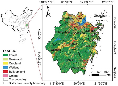
Zhejiang Province is one of the richest and most developed provinces in China (Zhao, Zhao, and Li 2019), and its economy has developed rapidly in recent years. From 2000 to 2018, GDP of Zhejiang increased by 13.09%, and exceeded 5,619.72 billion yuan in 2018. At the meantime, its proportion of urban population increased from 48.70% to 68.90%; the area of paved roads augmented from 90.50 to 459.46 million m²; and the amount of compound chemical fertilizer used for agriculture nearly doubled (Zhejiang Statistical Yearbook, 2001, 2019). However, intense human activities also posed great threats to the supply of ecosystem services. Therefore, we chose Zhejiang as our study area, aiming to provide guidance for the government to better manage the ecosystem–economy balance, and also set a good example of multi-objective ecosystem management for other fast-developing areas in China and the rest of the world.

Data collection and analysis

We chose 12 types of ecosystem service that are indispensable for human well-being, covering provisioning, regulating, cultural, and supporting services (Table 1), specifically including crop production, meat production, aquatic production, cotton production, fruit production, carbon sequestration, water retention, soil retention, forest recreation, tourism infrastructure, tourist population, and biodiversity. We also collected data of potential socioeconomic and natural factors related to ESBI variations, including GDP in 2000 and 2015, road density in 2000 and 2015, precipitation in 2000 and 2015, and so on (Table 2). We used administrative boundary (Ai et al. 2015; Li et al. 2017; Raudsepp-Hearne, Peterson, and Bennett 2010) of districts and counties to distinguish the research units. Due to data availability, we merged sub-administrative districts in the main urban areas of Hangzhou, Huzhou, Jinhua, Quzhou, and Jiaxing as separate larger research units, respectively. Meanwhile, we did not include island areas (i.e., Zhoushan City and Dongtou County of Wenzhou City) because of data scarcity for key indicators.

Table 1. Proxies used to measure 12 ecosystem services in Zhejiang Province

Ecosystem service (ES)	Proxies (2000 and 2015)	Data acquisition	Notes
Provisioning (ton/km^2)
Crop production (CP)	Yield of rice, yam, corn, beans and other cereals	Statistical Yearbooks of Hangzhou, Jinhua, Jiaxing, Ningbo, Wenzhou, Lishui, Taizhou and Shaoxing in 2001 and 2016; Statistical Yearbooks of Huzhou and Quzhou in 2016; Zhejiang Statistical Yearbook in 2001.	The main carbohydrate source
Meat production (MP)	Yield of beef, pork, mutton, rabbit and poultry		The main protein source
Aquatic production (AP)	Aquaculture and fishing products, including fish, shrimps, prawns, crabs, shellfish and others		The main aquatic protein source
Cotton production (COP)	The amount of cotton	Zhejiang Statistical Yearbook (2001 and 2016).	An important cash crop
Fruit production (FP)	The amount of fruit		An important source of vitamins and minerals
Regulating
Carbon sequestration (CS)	The amount of sequestered and stored carbon in terrestrial ecosystem (ton/km^2)	Research Center for Eco-Environmental Sciences, Chinese Academy of Sciences (Ouyang et al. 2016)	Important for carbon dioxide balance and climate change
Water retention (WR)	The water retention capacity of ecosystem (mm)		Indispensable for regional climate and agriculture
Soil retention (SR)	The soil retention capacity of the vegetation cover (ton/ha)		Important for ecosystem sustainability
Cultural
Forest recreation (FR)	The percentage of forest land (%)	Calculated from land use data at a 30-m resolution	A principal way to feel nature and refresh mind
Tourism infrastructure (TI)	Score of tourist attractions. S00 = N4A×5+ N3A×3, S15 = N5A×6+ N4A×5, where S00 and S15 represent the tourist attraction scores in 2000 and 2015; N5A, N4A, N3A are the number of AAAAA, AAAA, and AAA attractions, respectively.	China National Tourism Administration; Zhejiang Provincial Department of Culture and Tourism	A measurement of tourism infrastructure; the higher score represents better tourism infrastructure and services
Tourist population (TPOP)	The number of tourists (10^4 person)	Statistical Yearbooks and Yearbooks of 11 cities in Zhejiang (2001 and 2016)	A measurement of tourism attractiveness
Supporting
Biodiversity (BD)	The order of magnitude of vulnerable and endangered species	Obtained from Xu et al. (2017)	The importance level of biodiversity protection

Table 2. Potential factors related to change in ecosystem service bundle index

Category	Variables	Description
Natural	PREC00	Precipitation in 2000 (cm)
	PREC15	Precipitation in 2015 (cm)
	dPREC	Change in precipitation between 2000 and 2015 (cm)
	TEMP00	Annual temperature in 2000 (℃)
	TEMP15	Annual temperature in 2015 (℃)
	dTEMP	Change in annual temperature between 2000 and 2015 (℃)
Socioeconomic	GDP00	The GDP in 2000 (billion yuan)
	GDP15	The GDP in 2015 (billion yuan)
	dGDP	Change in GDP between 2000 and 2015 (billion yuan)
	GPAF00	Gross product of agriculture, forestry, animal husbandry and fishery (GPAF) in 2000 (100 million yuan)
	GPAF15	Gross product of agriculture, forestry, animal husbandry and fishery (GPAF) in 2015 (100 million yuan)
	dGPAF	Change in GPAF between 2000 and 2015 (100 million yuan)
	POP00	Total population in 2000 (10,000 person)
	POP15	Total population in 2015 (10,000 person)
	dPOP	Change in population between 2000 and 2015 (10,000 person)
	POPNA00	Non-agriculture population in 2000 (10,000 person)
	POPNA15	Non-agriculture population in 2015 (10,000 person)
	dPOPNA	Change in non-agriculture population between 2000 and 2015 (10,000 person)
	HN00	The number of households in 2000 (10,000 household)
	HN15	The number of households in 2015 (10,000 household)
	dHN	Change in household number between 2000 and 2015 (10,000 household)
	AREA00	Land area in 2000 (100 square kilometer)
	AREA15	Land area in 2015 (100 square kilometer)
	dAREA	Change in land area between 2000 and 2015 (100 square kilometer)
	EDU00	Education expenditure in 2000 (100 million yuan)
	EDU15	Education expenditure in 2015 (100 million yuan)
	dEDU	Change in education expenditure between 2000 and 2015 (100 million yuan)
	UR00	Urbanization rate in 2000 (%)
	UR15	Urbanization rate in 2015 (%)
	dUR	Change in urbanization rate between 2000 and 2015 (%)
	RD00	Road density in 2000 (100 m/km^2)
	RD15	Road density in 2015 (100 m/km^2)
	dRD	Change in road density between 2000 and 2015 (100 m/km^2)

We normalized the values of ecosystem service indicators in 2000 and 2015 together to 0 ~ 100 by the min-max normalization method to ensure comparability across years. Using the “corrplot” package in RStudio (version 1.1.383), we conducted the Spearman’s correlation analysis to demonstrate synergies and trade-offs among individual and diverse categories of ecosystem services. We constructed the ESBI system using Structural Equation Models (SEM) in Mplus (version 6.1) (Feng and Harring 2020). Then, we normalized the ESBI values and mapped their spatial distributions to show their spatiotemporal dynamics from 2000 to 2015.

SEM (Bollen & Noble, 2011) includes structural model and measurement model, and the general form of equations are as follows:

(1) ${\eta }_k={\alpha }_{\eta }+\mathrm{B}{\eta }_k+\mathrm{\Gamma }{\xi }_k+{\varsigma }_k$(1)

(2) $y_k={\alpha }_y+{\mathrm{\Lambda }}_y{\eta }_k+{\tau }_k$(2)

(3) $X_k={\alpha }_x+{\mathrm{\Lambda }}_x{\xi }_k+{\delta }_k$(3)

where formula (1) is the structural model, formula (2) and (3) are the measurement models. ${\xi }_k$ is the overall index of unit k; ${\eta }_k$ is the vector of sub-indices of unit k; ${\alpha }_{\eta }$, ${\alpha }_y$, ${\alpha }_x$ are intercept vectors; $\mathrm{B}$ is the correlation matrix among sub-indices; $\mathrm{\Gamma }$ is the weight matrix that sub-indices contributing to the overall index; $y_k$ and $X_k$ are the vectors of observing variables of ${\eta }_k$ and ${\xi }_k$, respectively; ${\mathrm{\Lambda }}_y$ and ${\mathrm{\Lambda }}_x$ are the weight matrices of $y_k$ to ${\eta }_k$ and $X_k$ to ${\xi }_k$, respectively; ${\varsigma }_k$, ${\tau }_k$ and ${\delta }_k$ are error terms.

In this study, the overall index is the ESBI; the sub-indices are ecosystem provisioning service set (EPS), ecosystem regulating service set (ERS), and ecosystem cultural service set (ECS); the observed variables are the 11 types of ecosystem service in Table 1 except biodiversity. We filtered observed variables for each sub-index based on the reliability test in Stata (version 14.1, StataCorp, College Station, Texas, USA), and modified the model by adding or removing paths between variables based on the modification indices and model fitness indices in Mplus. For the final model, the Comparative Fit Index (CFI) and Tucker–Lewis Index (TLI) often should be higher than 0.90; the Root Mean Square Error of Approximation (RMSEA) should be less than 0.08 (Wen and Liang 2015). Finally, we performed the multiple linear regression analyses to analyze factors associated with changes in ESBI values via R packages of “car” (Fox and Weisberg 2019) and “QuantPsyc” (Fletcher 2012). The dependent variable was the change in ESBI between 2000 and 2015, the independent variables are the initial value of ESBI and other factors shown in Table 2.

Results

Spatial and temporal distributions of ecosystem services

Supporting and most provisioning services had higher values in the northeast, central, and coastal areas of Zhejiang, and the output of aquatic products in coastal regions was particularly high (Figure 2). Carbon sequestration in the north was relatively lower than that in the central and southern areas; water retention was higher in the southwest and lower in the northeast; soil retention was higher in the northwest, south, and southeast, and lower in the northeast. The distribution of forest recreation was similar to that of soil retention; tourism infrastructure scattered in Zhejiang, and tourist population in the south lagged behind that in the north.

Figure 2. (a) Spatial distributions of ecosystem services for normalized crop production, meat production, aquatic production, cotton production, fruit production, and biodiversity in 2000 and 2015; (b) Spatial distributions of ecosystem services for normalized carbon sequestration, water retention, soil retention, forest recreation, tourism infrastructure and tourist population in 2000 and 2015

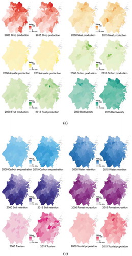
From 2000 to 2015, most provisioning services and all regulating, cultural, and supporting services improved (Table 3 and Figure 2). For provisioning services, fruit production increased most significantly, which was 3.86 times higher in 2015 than that in 2000, with obvious increases observed in the central, northeast, and coastal areas; crop and cotton production declined by 39.50% (4.85 million tons) and 26.08% (7,568.63 tons) respectively. Meanwhile, crop and cotton production were the only two with reduced overall outputs among the 12 ecosystem services. For regulating services, carbon sequestration increased the most (42.35%, 131.69 million tons), mainly distributed in the central, western, and southern regions. In contrast, water and soil retention increased only by 4.66% and 0.49%, and the latter changed the least among the 12 ecosystem services. For cultural services, tourism infrastructure and tourist population soared obviously. The average score of tourism infrastructure and the tourist population in 2015 were 15 times and 10 times of those in 2000, respectively. Tourist population in the middle and north increased faster than that in the south. For supporting service, biodiversity increased significantly in the whole province, with an average increase of 49.69% (0.80) in 76 districts and counties.

Table 3. Descriptive statistics of 12 ecosystem services in 2000 and 2015

Ecosystem services	District and county scale			Zhejiang Province
	Range2000	Range2015	Unit	2000	2015	Unit
CP	19.23 ~ 490.67	0 ~ 474.92	ton/km^2	12.28s	7.43s	Million ton
MP	1.84 ~ 75.55	0 ~ 107.39	ton/km^2	1.36s	1.64s	Million ton
AP	0.13 ~ 1016.41	0 ~ 933.33	ton/km^2	3.11s	3.98s	Million ton
COP	0 ~ 6.03	0 ~ 4.57	ton/km^2	29.02s	21.46s	Thousand ton
FP	0.64 ~ 151.28	3.27 ~ 936.57	ton/km^2	1.69s	8.21s	Million ton
CS	366.40 ~ 4062.69	43.00 ~ 5706.42	ton/km^2	310.98s	442.67s	Million ton
WR	405.25 ~ 1022.27	488.02 ~ 1079.10	mm	72.97s	77.63s	Billion m^3
SR	17.53 ~ 2037.26	18.44 ~ 2032.75	ton/ha	10.54s	10.59s	Billion ton
FR	0.66 ~ 88.94	0.71 ~ 89.84	%	61.61s	63.08s	%
TPOP	0.52 ~ 769.87	24.40 ~ 4012.03	10^4 person	73.17s	790.07s	Million person
TI	0 ~ 5.00	0 ~ 37.00	-	0.74 m (1.61)	11.03 m (8.03)	-
BD	1.09 ~ 3.14	1.68 ~ 3.79	-	1.61 m (0.44)	2.41 m (0.50)	-

(1) Range₂₀₀₀ and Range₂₀₁₅ refer to the ranges of ecosystem services at district and county levels before normalization in 2000 and 2015, respectively; (2) The subscripts of s and m refer to the sum value and the mean value, respectively; the numbers in the brackets are corresponding standard deviations; (3) CP, MP, AP, COP, FP, CS, WR, SR, FR, TI, TPOP and BD are abbreviations for crop production, meat production, aquatic production, cotton production, fruit production, carbon sequestration, water retention, soil retention, forest recreation, tourism infrastructure, tourist population, and biodiversity, respectively.

Trade-offs and synergies among ecosystem services

Among the 66 pairs of ecosystem services, 52 and 51 pairs were significantly correlated in 2000 and 2015, of which 27 and 30 pairs were highly correlated (Spearman’s coefficient [r] ≥ 0.5), and 18 and 20 pairs were moderately correlated (0.3 < r < 0.5) (Figure 3). In both years, there were positive correlations among individual services in categories of provisioning (p < 0.01) and regulating (p < 0.001), respectively. Tourism infrastructure and tourist population in cultural services were positively correlated (p < 0.05), representing apparent synergies. In terms of different categories of ecosystem service, regulating services were negatively correlated with both provisioning (p < 0.05) and supporting (p < 0.001) services, indicating obvious trade-offs. Forest recreation in cultural services had trade-off with provisioning services (p < 0.01), but had synergies with regulating services (p < 0.001). There were synergies between provisioning and supporting services (p < 0.01).

Figure 3. (a) and (b) refer to Spearman’s correlations between different ecosystem services in 2000 and 2015, respectively. Notes: Blue and red circles represent synergies and trade-offs, respectively. Values in the lower triangles are correlation coefficients. The higher the absolute values of correlation coefficients, the darker the color, the bigger the circle, and the stronger the correlation. CP, MP, AP, COP, FP, CS, WR, SR, FR, TI, TPOP, and BD are abbreviations for crop production, meat production, aquatic production, cotton production, fruit production, carbon sequestration, water retention, soil retention, forest recreation, tourism infrastructure, tourist population, and biodiversity, respectively. * p < 0.05, ** p < 0.01, *** p < 0.001

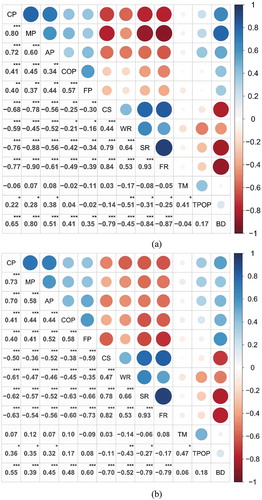
From 2000 to 2015, although the correlation direction was the same, the correlation degree changed, including 25 pairs of weakened ones and 22 pairs of enhanced ones. The synergies among crop, meat, and aquatic production weakened while the synergies between fruit production and meat, aquatic, cotton production enhanced. The trade-offs between crop, meat, aquatic production, and regulating services mostly became weaker, while the other two provisioning services’ trade-offs with regulating services enhanced. The synergy between tourism infrastructure and tourist population strengthened. Except cotton, fruit production, and water retention, the relationships between biodiversity with other services weakened.

ESBI system and its spatiotemporal dynamics

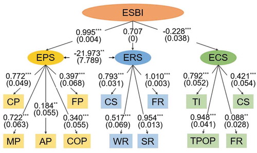
As Figure 4 shows, ESBI overall index was significantly measured by three sub-indices: EPS, ERS, and ECS. The coefficients of EPS and ERS were both positive, while that of ECS was negative and the correlation between EPS and ERS was negative. The EPS had the greatest influence on ESBI, while the ECS had the least. The standardized coefficients of all indicators for sub-indices were positive (p < 0.01). EPS was measured by five provisioning services, of which the contributions of crop (standardized coefficient [SC] = 0.772) and meat production (SC = 0.722) were relatively high and that of aquatic production was the lowest. ERS was explained by three regulating services and one cultural service (forest recreation). Forest recreation contributed the most (SC = 1.010), while water retention the least. ECS was estimated by three cultural services and one regulating service (carbon sequestration), with the largest contribution of tourist population (SC = 0.948) and the smallest of forest recreation.

Figure 4. Ecosystem service bundle index components path diagram. Notes: (1) N = 149; Comparative Fit Index (CFI): 0.993, Tucker-Lewis Index (TLI): 0.984, Root Mean Square Error of Approximation (RMSEA): 0.043, Standardized Root Mean Square Residual (SRMR): 0.039; (2) *p < 0.05, **p < 0.01, ***p < 0.001; (3) the unstandardized coefficient of ERS was fixed as 1; (4) coefficients in the diagram are standardized with corresponding standard errors are in brackets; and (5) ESBI, EPS, ERS, and ECS represent the ecosystem service bundle index, ecosystem provisioning service set, ecosystem regulating service set, and ecosystem cultural service set, respectively; CP, MP, AP, COP, FP, CS, WR, SR, FR, TI, and TPOP are abbreviations for crop production, meat production, aquatic production, cotton production, fruit production, carbon sequestration, water retention, soil retention, forest recreation, tourism infrastructure, and tourist population, respectively. Please see more details in Appendix A

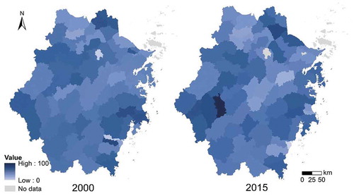
The spatial pattern of ESBI in 2000 was similar with that in 2015 (Figure 5), with higher ESBI values in the north central, west, and southeast, lower values in the northwest corner and central areas. From 2000 to 2015, the ESBI values of 25 districts/counties increased, mainly distributed in the Middle West, and those of 48 decreased, mainly situated in the Middle East. Compared to 2000, the spatial distribution of ESBI in 2015 was more uneven, with the standard deviation increased by 14.15% from 13.57 to 15.49, and the average decreased by 3.10% from 40.98 to 39.71.

Figure 5. Spatial patterns of ESBI in Zhejiang Province in 2000 and 2015. Notes: The ranges of ESBI values in 2000 and 2015 were 0.78 ~ 72.57 and 0 ~ 100, respectively

Factors associated with changes in ESBI

Table 4 shows the descriptive statistics of variables used for the construction of regression models. Table 5 shows that eight variables, covering initial value, socioeconomic, and natural factors, explained 48.63% of the total variance for the increase in ESBI. Change in precipitation (SC = 0.627, p < 0.05) was significantly related to the increase of ESBI. ESBI in 2000 (SC = −0.461, p < 0.1), change in household number (SC = 0.657, p < 0.1), precipitation in 2000 (SC = 0.719, p < 0.1), and annual temperature in 2000 (SC = 0.655, p < 0.1) were marginally significant in estimating the increase of ESBI. Road density in 2000, household numbers in 2000, and education expenditure in 2000 were not significantly relevant to the increase of ESBI.

Table 4. Summary statistics of explanatory variables used for regression models

Category	Variables	Mean (Standard deviation)
		Increase	Decrease
Socioeconomic	ESBIN00	35.96 (11.94)	45.07 (12.00)
	lnGDP00	2.03 (0.74)	1.62 (0.94)
	GPAF00	17.78 (8.56)	12.22 (9.02)
	dGPAF	28.04 (17.25)	19.46 (15.23)
	RD00	1.83 (0.53)	1.88 (0.47)
	dRD	1.53 (0.65)	1.33 (0.86)
	HN00	21.13 (10.31)	17.24 (9.53)
	dHN	3.85 (4.05)	2.09 (2.52)
	EDU00	0.98 (0.72)	0.80 (0.45)
	UR00	24.86 (18.92)	17.11 (9.89)
Natural	PREC00	153.47 (26.69)	166.93 (28.61)
	dPREC	39.97 (33.09)	15.64 (38.89)
	TEMP00	16.32 (0.51)	16.25 (0.61)
	dTEMP	1.34 (0.92)	1.78 (1.09)

Table 5. Effects of factors associated with the increase in ESBI

Category	Factor	Unstandardized Coefficients	Std. Error	Standardized Coefficients	t value
Socioeconomic	ESBIN00	−0.561^†	0.319	−0.461^†	−1.762
	RD00	−11.686	8.180	−0.426	−1.429
	HN00	−0.095	0.521	−0.067	−0.182
	dHN	2.361^†	1.243	0.657^†	1.900
	EDU00	−17.554	10.057	−0.867	−1.746
Natural	PREC00	0.392^†	0.204	0.719^†	1.925
	dPREC	0.276*	0.125	0.627*	2.210
	TEMP00	18.704^†	9.845	0.655^†	1.900
Intercept		−312.236	183.119	-	−1.705

Dependent variable is the normalized value of ecosystem service bundle index in 2015 minus that of 2000. N = 25; R² = 0.486. ^† p < 0.1, * p < 0.05, ** p < 0.01, *** p < 0.001.

Table 6 suggests that eleven factors, including initial value, socioeconomic, and natural factors, collectively explained 74.64% of the total variance for the decrease in ESBI. Except road density in 2000 and natural factors, the other seven factors were statistically significant associated with the decrease in ESBI. According to standardized coefficients, household numbers in 2000 contributed the most across the model (SC = 1.302, p < 0.001), followed by GDP in 2000 (SC = −1.260, p < 0.001), gross product of agriculture, forestry, animal husbandry, and fishery (GPAF) in 2000 (SC = −0.705, p < 0.01), change in road density (SC = −0.524, p < 0.001), change in GPAF (SC = 0.482, p < 0.05), and urbanization rate in 2000 (SC = 0.418, p < 0.01). ESBI in 2000 (SC = −0.290, p < 0.01) contributed the least.

Table 6. Effects of factors associated with the decrease in ESBI

Category	Factor	Unstandardized Coefficients	Std. Error	Standardized Coefficients	t value
Initial value	ESBIN00	−0.238**	0.074	−0.290**	−3.221
Socioeconomic	lnGDP00	−13.211***	2.531	−1.260***	−5.220
	GPAF00	−0.770**	0.262	−0.705**	−2.936
	dGPAF	0.311*	0.131	0.482*	2.372
	RD00	−1.983	2.068	−0.094	−0.959
	dRD	−5.985***	1.651	−0.524***	−3.625
	HN00	1.344***	0.228	1.302***	5.893
	UR00	0.416**	0.133	0.418**	3.136
Natural	PREC00	−0.108	0.064	−0.315	−1.685
	TEMP00	0.115	2.616	0.007	0.044
	dTEMP	−1.404	1.586	−0.156	−0.885
Intercept		25.725	39.194	-	0.656

Dependent variable is the normalized value of ecosystem service bundle index in 2015 minus that of 2000. N = 48; R² = 0.746. ^† p < 0.1, * p < 0.05, ** p < 0.01, *** p < 0.001.

Discussion

We selected 12 key ecosystem services in Zhejiang Province, displayed the spatiotemporal dynamics (between 2000 and 2015), and explored their potential synergies and trade-offs. Then, to explore the overall status of ecosystem services, we constructed the ESBI system and further analyzed the factors associated with changes in ESBI values. Below we compared our results with those of existing literature, summarized advantages and limitations of our study, and provided some insights for future research and management.

We found that at individual service level, provisioning services were synergistic with each other and so were regulating services; however, at the grouped service level, provisioning services had trade-offs with regulating services. These results were in line with those of Zhang et al. (2016), Xu et al. (2016), and Jia et al. (2014), but different from Lyu et al. (2019) and Ai et al. (2015). Such a discrepancy is probably due to the complexity of ecosystem service relationship, which is affected by ecosystem type, selected service indicator, ecosystem service assessment method, geographic and climate conditions, and other factors. Furthermore, in line with Yang et al. (2015a) and Lyu et al. (2019), our results suggest that there is no agreement on the relationships between cultural services and other services. Biodiversity in our study had trade-off with soil retention, and this viewpoint is consistent with Sun and Li (2017), who estimated the relationship of soil conservation and biodiversity protection in Zengcheng District, Guangzhou City. However, Liu, Xu, and Jiang (2015) found that soil retention and biodiversity protection are synergistic in Wangqing County, Yanbian Autonomous Prefecture, Jilin Province. Biodiversity has synergies with provisioning services in our study may because plantations where most provisioning services are produced also provide food and habitats for vulnerable and endangered animals and plants (Cox et al. 2006; Fang 2017; Schmid 2002).

Our proposed ESBI system has several advantages in understanding relationships among multiple ecosystem services. The higher the ESBI values, the more synergies and the less trade-offs exist in the corresponding analysis units, the better aggregated ecosystem service provision, and vice versa. The increase in ESBI is beneficial while the decrease in ESBI is harmful. The advantages of our proposed ESBI system are as follows. First, as long as data are sufficient, our system can be applied to study areas at different scales. It provides possibility for other regions to study the aggregated pattern of ecosystem services at the scale of country, city, town, and even pixel. Second, it is a composite index system, including both the overall index and sub-indices. One can not only display the distribution of ESBI but also grasp the pattern of each sub-index. Third, the weighting of both overall index and sub-indices are objective and unequal. They are determined by the variation of data. If needed, one may also customize the weighting of any index by fixing its corresponding coefficient in the structural equation model (Yang, McKinnon, and Turner 2015c). Therefore, it is flexible and feasible for different management purposes such as providing most aggregated ecosystem services, providing most provisioning services, or developing tourism and minimizing the impacts on regulating services. Fourthly, the values of computed ESBI are continuous rather than categorical, and thus are easily available for further quantitative analyses. Finally, in contrast to monetizing all selected ecosystem services, our proposed ESBI system provides an alternative non-monetary solution to assess the aggregated pattern and relationships of multiple ecosystem services. Thus, our approach also avoids the disputes on discrepancy of different economic valuation methods (Yang et al. 2008).

There are also some limitations in our study. First, although we have taken data quality control measures, our results may be influenced to some extent due to the data scarcity and potential errors in some of our selected indicators obtained from government statistic yearbooks. Second, ecosystem service patterns may be dependent on the indicators used. For example, results may be different when taking forest land proportion and the number of hunting animals as the proxies of forest recreation service. Third, positive and negative correlations between ecosystem services suggest potential synergies and trade-offs, respectively. Fourth, we did not include policy factors in determining the drivers of changes in ESBI values.

We identified several issues for further research. First, it would be helpful to better understand the impacts of cultural services on overall ecosystem by dividing tourism attractions into different categories, such as natural spots, historic relics, and wildlife spots. Second, it would be interesting to understand how policy factors may influence the relationships among multiple ecosystem services as well as the ESBI values as a whole. Finally, future research may also use the overall index and sub-indices of ESBI for further analyses such as hotspot/coldspot identification, spatial planning, and priority settings for conservation and development.

Conclusions

We mapped the distributions of 12 ecosystem services in 2000 and 2015, analyzed the relationships among ecosystem services by Spearman’s correlation analysis, constructed ecosystem service bundle index system via structural equation model, and explored driving forces of ESBI spatiotemporal variations using multiple linear regression. Our main findings include: (1) most ecosystem services were spatially clustered. There were synergies between individual ecosystem services in categories of provisioning and regulating services, respectively. Regulating services had trade-offs with both provisioning and supporting services, while there were synergies between the latter two categories; (2) Our proposed ESBI index system consists of overall index and sub-indices of provisioning, regulating, and cultural services. The higher the ESBI value, the more important the corresponding place for multiple aggregated ecosystem service provision. ESBI overall indices were higher in the north central, west, and southeast, and lower in the northwest corner and central areas. Compared to 2000, ESBI in 2015 distributed more unevenly, and the average dropped by 3.10%; and (3) the increase of ESBI was associated with the initial value, and four socioeconomic and natural factors; the decrease of ESBI was influenced by the initial value and six socioeconomic factors. Our study may give guidance to better realize multi-objective ecosystem service management and lay a solid foundation for further study.

Author contributions

W.Y. designed the research; Y.H. collected and compiled the data, and conducted the analysis; Y.H. and W.Y. wrote the first draft; all authors revised the manuscript together. The authors declare no competing financial interests.

Additional information

Funding

This work was supported by the National Natural Science Foundation of China [Grant number 71673247]; Ministry of Science and Technology of China [Grant number 2016YFC0503404]; and Outstanding Youth Fund of Zhejiang Province [Grant number LR18D010001].

Appendix A.

Structural equation model results of the ecosystem service bundle index system

Overall index	Sub-indices	Indicators	Unstandardized coefficients		Standardized coefficients
			Coefficients	Standard error	Coefficients	Standard error
ESBI	EPS		9.499**	3.358	0.995***	0.004
		CP	0.080**	0.028	0.772***	0.049
		MP	0.076**	0.026	0.722***	0.063
		AP	0.019*	0.010	0.184**	0.055
		COP	0.033*	0.014	0.340***	0.055
		FP	0.030*	0.013	0.397***	0.068
	ERS		1.000	0	0.707	0
		CS	0.539***	0.046	0.793***	0.031
		WR	0.366***	0.052	0.517***	0.069
		SR	0.664***	0.031	0.954***	0.013
		FR	0.697***	0.029	1.010***	0.003
	ECS		−0.234***	0.041	−0.228***	0.038
		TI	0.764***	0.091	0.792***	0.052
		TPOP	0.907***	0.103	0.948***	0.041
		FR	0.083**	0.026	0.088**	0.028
		CS	0.394***	0.045	0.421***	0.054

(1) N = 149; Comparative Fit Index (CFI): 0.993, Tucker-Lewis Index (TLI): 0.984, Root Mean Square Error of Approximation (RMSEA): 0.043, Standardized Root Mean Square Residual (SRMR): 0.039; (2) * p < 0.05, ** p < 0.01, *** p < 0.001; (3) the coefficient of ERS was fixed as 1. The EPS and ERS was negatively correlated with a coefficient of −21.973 and standard error of 7.789 (p < 0.01); and (4) ESBI, EPS, ERS, and ECS represent the ecosystem service bundle index, ecosystem provisioning service set, ecosystem regulating service set, and ecosystem cultural service set, respectively; CP, MP, AP, COP, FP, CS, WR, SR, FR, TI, and TPOP are abbreviations for crop production, meat production, aquatic production, cotton production, fruit production, carbon sequestration, water retention, soil retention, forest recreation, tourism infrastructure, and tourist population, respectively.

References

- Ai, J., X. Sun, L. Feng, Y. Li, and X. Zhu. 2015. “Analyzing the Spatial Patterns and Drivers of Ecosystem Services in Rapidly Urbanizing Taihu Lake Basin of China.” Frontiers of Earth Science 9 (3): 531–14. doi:10.1007/s11707-014-0484-1.
- Bollen, K. A., and M. D. Noble. 2011. “Structural Equation Models and the Quantification of Behavior.” Proceedings of the National Academy of Sciences of the United States of America 108: 15639–15646. doi:10.1073/pnas.1010661108.
- Cox, S. B., C. P. Bloch, R. D. Stevens, and L. F. Huenneke. 2006. “Productivity and Species Richness in an Arid Ecosystem: A Long-term Perspective.” Plant Ecology 186 (1): 1–12. doi:10.1007/s11258-006-9107-6.
- Crouzat, E., M. Mouchet, F. Turkelboom, C. Byczek, J. Meersmans, F. Berger, P. J. Verkerk, S. Lavorel, and T. Diekötter. 2015. “Assessing Bundles of Ecosystem Services from Regional to Landscape Scale: Insights from the French Alps.” Journal of Applied Ecology 52 (5): 1145–1155. doi:10.1111/1365-2664.12502.
- Dittrich, A., R. Seppelt, T. Václavík, and A. F. Cord. 2017. “Integrating Ecosystem Service Bundles and Socio-environmental Conditions – A National Scale Analysis from Germany.” Ecosystem Services 28: 273–282. doi:10.1016/j.ecoser.2017.08.007.
- Fang, Y. 2017. “Protection of Rural and Agricultural Biodiversity - A Case Study of Jiangsu Province.” Shangpin Yu Zhiliang 2017 (38): 22–23. doi:10.3969/j.issn.1006-656X.2017.38.015.
- Feng, Y., and J. R. Harring. 2020. “Structural Equation Modeling: Applications Using Mplus.” Psychometrika 85 (2): 526–530. doi:10.1007/s11336-020-09706-5.
- Fletcher, T. D. 2012. “QuantPsyc: Quantitative Psychology Tools.” https://cran.r-project.org/web/packages/QuantPsyc/index.html
- Fox, J., and S. Weisberg. 2019. “Car: Companion to Applied Regression.” https://cran.r-project.org/web/packages/car/index.html
- Haines-Young, R., and M. Potschin-Young. 2018. “Revision of the Common International Classification for Ecosystem Services (CICES V5.1): A Policy Brief.” One Ecosystem 3: e27108. doi:10.3897/oneeco.3.e27108.
- Jia, X., B. Fu, X. Feng, G. Hou, Y. Liu, and X. Wang. 2014. “The Tradeoff and Synergy between Ecosystem Services in the Grain-for-Green Areas in Northern Shaanxi, China.” Ecological Indicators 43: 103–113. doi:10.1016/j.ecolind.2014.02.028.
- Jiang, C., and L. Zhang. 2016. “Ecosystem Change Assessment in the Three-river Headwater Region, China: Patterns, Causes, and Implications.” Ecological Engineering 93: 24–36. doi:10.1016/j.ecoleng.2016.05.011.
- Kim, I., S. Kim, J. Lee, and H. Kwon. 2018. “Analysis on Ecosystem Service Hotspots Based on Regional Environmental Stakeholders’ Perception – A Case Study of Ansan –.” Journal of Environmental Impact Assessment 27 (5): 417–430.
- Li, H., J. Peng, Y. Hu, and W. Wu. 2017. “Ecological Function Zoning in Inner Mongolia Autonomous Region Based on Ecosystem Service Bundles.” Chinese Journal of Applied Ecology 28 (8): 2657–2666. doi:10.13287/j.1001-9332.201708.036.
- Li, H., Z. Ren, Y. Liu, and J. Zhang. 2016a. “Tradeoffs-synergies Analysis among Ecosystem Services in Northwestern Valley Basin: Taking Yinchuan Basin as an Example.” Journal of Desert Research 36 (6): 1731–1738. doi:0.7522/j.issn.1000-694X.2016.00049.
- Li, J., H. Li, and L. Zhang. 2016b. “Ecosystem Service Trade-offs in the Guanzhong-Tianshui Economic Region of China.” Acta Ecologica Sinica 36 (10): 3053–3062. doi:10.5846/stxb201408261688.
- Li, Z., Z. Sun, Y. Tian, J. Zhong, and W. Yang. 2019. “Impact of Land Use/Cover Change on Yangtze River Delta Urban Agglomeration Ecosystem Services Value: Temporal-Spatial Patterns and Cold/Hot Spots Ecosystem Services Value Change Brought by Urbanization.” International Journal of Environmental Research and Public Health 16 (1): 1–18. doi:10.3390/ijerph16010123.
- Ling, H., J. Yan, H. Xu, B. Guo, and Q. Zhang. 2019. “Estimates of Shifts in Ecosystem Service Values Due to Changes in Key Factors in the Manas River Basin, Northwest China.” Science of the Total Environment 659: 177–187. doi:10.1016/j.scitotenv.2018.12.309.
- Liu, L., H. Zhang, Y. Gao, W. Zhu, X. Liu, and Q. Xu. 2019. “Hotspot Identification and Interaction Analyses of the Provisioning of Multiple Ecosystem Services: Case Study of Shaanxi Province, China.” Ecological Indicators 107: 1–13. doi:10.1016/j.ecolind.2019.105566.
- Liu, Y., G. Xu, and H. Jiang. 2015. “Synergy between Ecosystem Services and Ecosystem Health in the Forest Area of Northeast China.” Progress in Geography 34 (6): 761–771. doi:10.18306/dlkxjz.2015.06.011.
- Lyu, R., K. C. Clarke, J. Zhang, J. Feng, X. Jia, and J. Li. 2019. “Spatial Correlations among Ecosystem Services and Their Socio-ecological Driving Factors: A Case Study in the City Belt along the Yellow River in Ningxia, China.” Applied Geography 108: 64–73. doi:10.1016/j.apgeog.2019.05.003.
- MA. 2005. Ecosystems & Human Well-being: Synthesis Millennium Ecosystem Assessment). Washington, DC: Island Press.
- Mouchet, M. A., M. L. Paracchini, C. J. E. Schulp, J. Stürck, P. J. Verkerk, P. H. Verburg, and S. Lavorel. 2017. “Bundles of Ecosystem (Dis)services and Multifunctionality across European Landscapes.” Ecological Indicators 73: 23–28. doi:10.1016/j.ecolind.2016.09.026.
- Ouyang, Z., H. Zheng, Y. Xiao, S. Polasky, J. Liu, W. Xu, Q. Wang, et al.. 2016. “Improvements in Ecosystem Services from Investments in Natural Capital.” Science 352 (6292): 1455–1459. doi:10.1126/science.aaf2295.
- Qin, K., J. Li, and X. Yang. 2015. “Trade-Off and Synergy among Ecosystem Services in the Guanzhong-Tianshui Economic Region of China.” International Journal of Environmental Research and Public Health 12 (11): 14094–14113. doi:10.3390/ijerph121114094.
- Qiu, J. X., and M. G. Turner. 2013. “Spatial Interactions among Ecosystem Services in an Urbanizing Agricultural Watershed.” Proceedings of the National Academy of Sciences of the United States of America 110 (29): 12149–12154. doi:10.1073/pnas.1310539110.
- Ran, F., Z. Luo, J. Wu, S. Qi, L. Cao, Z. Cai, and Y. Chen. 2019. “Spatiotemporal Patterns of the Trade-off and Synergy Relationship among Ecosystem Services in Poyang Lake Region, China.” Chinese Journal of Applied Ecology 30 (3): 995–1004. doi:10.13287/j.1001-9332.201903.005.
- Raudsepp-Hearne, C., G. D. Peterson, and E. M. Bennett. 2010. “Ecosystem Service Bundles for Analyzing Tradeoffs in Diverse Landscapes.” Proceedings of the National Academy of Sciences of the United States of America 107 (11): 5242–5247. doi:10.1073/pnas.0907284107.
- Renard, D., J. M. Rhemtulla, and E. M. Bennett. 2015. “Historical Dynamics in Ecosystem Service Bundles.” Proceedings of the National Academy of Sciences of the United States of America 112 (43): 13411–13416. doi:10.1073/pnas.1502565112.
- Roces-Diaz, J. V., J. Vayreda, M. Banque-Casanovas, M. Cuso, M. Anton, J. A. Bonet, L. Brotons, et al.. 2018. “Assessing the Distribution of Forest Ecosystem Services in a Highly Populated Mediterranean Region.” Ecological Indicators 93: 986–997. doi:10.1016/j.ecolind.2018.05.076.
- Schirpke, U., S. Candiago, L. E. Vigl, H. Jäger, A. Labadini, T. Marsoner, C. Meisch, E. Tasser, and U. Tappeiner. 2019. “Integrating Supply, Flow and Demand to Enhance the Understanding of Interactions among Multiple Ecosystem Services.” Science of the Total Environment 651: 928–941. doi:10.1016/j.scitotenv.2018.09.235.
- Schmid, B. 2002. “The Species Richness–productivity Controversy.” TRENDS in Ecology & Evolution 17 (3): 113–114. doi:10.1016/S0169-5347(01)02422-3.
- Seto, K. C., B. Guneralp, and L. R. Hutyra. 2012. “Global Forecasts of Urban Expansion to 2030 and Direct Impacts on Biodiversity and Carbon Pools.” Proceedings of the National Academy of Sciences 109 (40): 16083–16088. doi:10.1073/pnas.1211658109.
- Sun, X., and F. Li. 2017. “Spatiotemporal Assessment and Trade-offs of Multiple Ecosystem Services Based on Land Use Changes in Zengcheng, China.” Science of the Total Environment 609: 1569–1581. doi:10.1016/j.scitotenv.2017.07.221.
- Turner, K. G., M. V. Odgaard, P. K. Bocher, T. Dalgaard, and J.-C. Svenning. 2014. “Bundling Ecosystem Services in Denmark: Trade-offs and Synergies in a Cultural Landscape.” Landscape and Urban Planning 125: 89–104. doi:10.1016/j.landurbplan.2014.02.007.
- Wang, C., S. Wang, B. Fu, Z. Li, X. Wu, and Q. Tang. 2017. “Precipitation Gradient Determines the Tradeoff between Soil Moisture and Soil Organic Carbon, Total Nitrogen, and Species Richness in the Loess Plateau, China.” Science of the Total Environment 575: 1538–1545. doi:10.1016/j.scitotenv.2016.10.047.
- Wen, H., and Y. Liang. 2015. “The Essence of Testing Structural Equation Models Using Popular Fit Indexes.” Journal of Psychological Science 38 (4): 987–994. doi:10.16719/j.cnki.1671-6981.2015.04.031.
- Wu, J., X. Zhong, J. Peng, and W. Qin. 2015. “Function Classification of Ecological Land in a Small Area Based on Ecosystem Service Bundles: A Case Study in Liangjiang New Area, China.” Acta Ecologica Sinica 35 (11): 3808–3816. doi:10.5846/stxb201408081581.
- Wu, J., Z. Feng, Y. Gao, and J. Peng. 2013. “Hotspot and Relationship Identification in Multiple Landscape Services: A Case Study on an Area with Intensive Human Activities.” Ecological Indicators 29: 529–537. doi:10.1016/j.ecolind.2013.01.037.
- Xu, W., Y. Xiao, J. Zhang, W. Yang, L. Zhang, V. Hull, Z. Wang, et al.. 2017. “Strengthening Protected Areas for Biodiversity and Ecosystem Services in China.” Proceedings of the National Academy of Sciences of the United States of America 114 (7): 1601–1606. doi:10.1073/pnas.1620503114.
- Xu, Y., H. Tang, B. Wang, and J. Chen. 2016. “Effects of Land-use Intensity on Ecosystem Services and Human Well-being: A Case Study in Huailai County, China.” Environmental Earth Sciences 75 (5): 1–11. doi:10.1007/s12665-015-5103-2.
- Yang, G., and W. Tuo. 2002. “Sandstorm Disasters and Controlling Ways in the Agricultural and Pasturing Interlaced Zone of Ningxia, Inner Mongolia and Shaanxi.” Journal of Desert Research 22 (5): 452–465.
- Yang, G., Y. Ge, H. Xue, W. Yang, Y. Shi, C. Peng, Y. Du, X. Fan, Y. Ren, and J. Chang. 2015a. “Using Ecosystem Service Bundles to Detect Trade-offs and Synergies across Urban–rural Complexes.” Landscape and Urban Planning 136: 110–121. doi:10.1016/j.landurbplan.2014.12.006.
- Yang, W., J. Chang, B. Xu, C. Peng, and Y. Ge. 2008. “Ecosystem Service Value Assessment for Constructed Wetlands: A Case Study in Hangzhou, China.” Ecological Economics 68 (1–2): 116–125. doi:10.1016/j.ecolecon.2008.02.008.
- Yang, W., M. McKinnon, and W. Turner. 2015c. “Quantifying Human Well-being for Sustainability Research and Policy.” Ecosystem Health and Sustainability 1 (4): 4. doi:10.1890/ehs15-0004.1.
- Yang, W., T. Dietz, D. Kramer, Z. Ouyang, and J. Liu. 2015b. “An Integrated Approach to Understanding the Linkages between Ecosystem Services and Human Well-being.” Ecosystem Health and Sustainability 1 (5): 5. doi:10.1890/ehs15-0001.1.
- Yao, J., X. He, W. Chen, Y. Ye, R. Guo, and L. Yu. 2016. “A Local-scale Spatial Analysis of Ecosystem Services and Ecosystem Service Bundles in the Upper Hun River Catchment, China.” Ecosystem Services 22: 104–110. doi:10.1016/j.ecoser.2016.09.022.
- Zhang, Z., J. Gao, X. Fan, M. Zhao, and Y. Lan. 2016. “Assessing the Variable Ecosystem Services Relationships in Polders over Time: A Case Study in the Eastern Chaohu Lake Basin, China.” Environmental Earth Sciences 75 (10): 1–13. doi:10.1007/s12665-016-5683-5.
- Zhao, T., Y. Zhao, and M.-H. Li. 2019. “Landscape Performance for Coordinated Development of Rural Communities & Small-Towns Based on “Ecological Priority and All-Area Integrated Development”: Six Case Studies in East China’s Zhejiang Province.” Sustainability 11: 15. doi:10.3390/su11154096.
- Zhejiang Statistics Bureau. 2001. Zhejiang Statistical Yearbook. Beijing: China Statistics Press.
- Zhejiang Statistics Bureau. 2016. Zhejiang Statistical Yearbook. Beijing: China Statistics Press
- Zhejiang Statistics Bureau. 2019. Zhejiang Statistical Yearbook. Beijing: China Statistics Press.