How urbanization affect the ecosystem health of Tibet based on terrain gradients: a case study of Shannan, China

ABSTRACT

Urbanization has significant impacts on ecosystem health (ESH) by affecting land-use patterns. The evaluation of the ESH and the spatial correlations between human interference provides an insight into sustainable development as a response to potential ecological degradation if ESH is threatened by further urbanization. We applied the Vigor-Organization-Resilience-Services (VORS) modelto detect the responses of ESH of Shannan Prefecture in the Tibet to urbanization from 1990 to 2015, based on different levels of terrain gradients. The results show that the ESH of the most areas in Shannan reaches the levels of highest health and average health during the study period. By 2015, the area proportion at the highest health level increased by 0.68%, while that of degraded level decreased by 1.51%. Overall, the ESH of areas tends to shrink at higher-level TGs, and urban sprawl with ESH shrinking existed in middle-level TGs in Shannan. Furthermore, a significant spatial aggregation effect was found concerning that low ESH–high CUL type is mainly distributed on the middle-level TGs with dense human population. The results highlight the needs to rationally organize urbanization process in plateau regions based on different TGs, which contribute to maintain ESH advancing people livelihood improvement.

KEYWORDS:

• Ecosystem health
• terrain gradient
• urbanization
• spatial correlation
• Shannan

Introduction

Ecosystem health (ESH) is a comprehensive characteristic of the ecosystem, which can be considered as the integrity of ecosystem structure and function under the interference of human activities (Rapport, Costanza, and McMichael 1998; Costanza, Norton, and Haskell 1992; Lv et al. 2015). ESH evaluation is an effective approach for measuring ecosystem fragmentation and stability (Peng et al. 2015; Kang et al. 2018; Wu et al. 2021), as well as sustainability (Lv et al. 2015). In the past few decades, a significant progress has been made in ESH research. Previous studies were focusing on grassland ESH (Zhao et al. 2017), watershed ESH (Cao and Li 2018; Wen et al. 2021), wetland ESH (Sun et al. 2016), coastal ESH (Kim and Xu 2014), cultivated land ESH (Li, Qin, and Gao 2006), and urban ESH (Su, Fath, and Yang 2010; Li et al. 2021). In terms of the evaluation methods, more researches preferred using indicator system methods to evaluate ESH, including VOR (Vigor-Organization-Resilience) (Costanza, Norton, and Haskell 1992) and its extend version Vigor-Organization-Resilience-Services (VORS) model (Peng et al. 2015; Li et al. 2021), Pressure-State-Response (PSR) model (Zhao et al. 2021), and Driving-Pressure-State-Impact-Response (DPSIR) model (Fu, Chen, and Li 2009; Hou et al. 2014). These case studies demonstrated that urbanization has significant impacts on ESH, and the VORS model has been widely applied to assess ESH of the regions with different urbanization levels in China.

Different from the urbanized areas in urban agglomerations, the Qinghai-Tibet Plateau, which are suffering from serious environmental deterioration brought by both climate change and human interventions, is more vulnerable to the impacts of urbanization with attracting less attentions (Jiang et al. 2021; Xiao et al. 2021). Current studies on this ecologically vulnerable area mainly focus on ecological risk assessment through land-use analysis (Fayiah et al. 2020) and less highlight the relationships between urbanization and ESH from a holistic view. Undeniably, sustainable urbanization contributes to a healthy ecosystem, which is fundamental to maintain the survival of human society, especially for human well-being in Qinghai-Tibet Plateau (Li et al. 2021). The Plateau has the highest average elevation among the major plateau areas worldwide, and the high altitude and harsh environmental condition of which make it turn to be most fragile alpine ecosystem (Xiao et al. 2021). As the main component of the Qinghai-Tibet Plateau, Tibet Plateau generally is not regarded as an ideal place for urbanization, but it is the core part for the implementation of “China Western Development Strategy” (NPC (The National People’s Congress of the People’s Republic of China) 2013), which may face severer ecological and environmental problems in coming years with accelerated urbanization promoted by “Promoting Urbanization Strategy” (Xian et al. 2019). Therefore, the studies concerning differences in the responses of regional ESH to urbanization in Tibet are warranted.

Landscape pattern is the important factor influencing ESH (Peng et al. 2015), and the terrain gradient (TG) plays a more essential role in the ecological assessment of Qinghai-Tibet Plateau as illustrated above (Han, Yu, and Chen 2021). We have taken Shannan Prefecture in Tibet as a case study as it is a typical plateau mountainous area with large altitude differences and diverse ecosystem types, which is very important for the ecological security of the Tibet and even China (Zhang et al. 2021). Meanwhile, Shannan Prefecture experienced rapid urbanization, and the growth rate of GDP reached 7.9% by 2020, ranking the second in the Tibet (Shannan Municipal Statistics Bureau 2021). Therefore, Shannan Prefecture is an ideal study site for exploring the responses of ESH to urbanization in Tibet since the increase in human activities drove by economic urbanization has a significant impact on the ESH (Ouyang, Zhu, and He 2020; Shen et al. 2020). To identify the long-term impact of urbanization on the ESH of plateau, the main objectives of this study were to (i) describe the land-use changing based on TGs during 1990–2015, (ii) reveal the spatial variation of ESH on different TGs, and (iii) analyze the spatial correlations between ESH and urbanization, which are conductive to formulating reasonable land policies to balance urbanization and ESH for Tibet plateau and beyond.

Materials and methods

Study area

Shannan Prefecture is situated in the middle and lower reaches of Brahmaputra River and the south-central part of Tibet Autonomous Region (90°14’-94°22ʹE, 27°08’-29°47ʹN), which runs through the eastern section of the Himalayas (Figure 1). The territory is quite large, with a total area of 79,300 km², bordering India and Bhutan. Shannan is the birthplace of Tibetan culture with a percentage of Tibetan population reaching 90% (Tibet Autonomous Region Bureau of Statistics 2021). There are obvious rainy and dry seasons influenced by semi-arid monsoon climate throughout the year with an annual precipitation fluctuating between 200 and 500 mm. The elevation of the whole region fluctuates greatly; the terrains present higher in the north and lower in the south. The average altitude is above 3700 m, and the terrain gradient ranges from 0 to 2.5352, which can normally be classified into five levels for topographic analysis based on elevation and slope (Gong et al. 2017; Shi, Han, and Guo 2020). In recent years, the economic development of Shannan was accelerated by urbanization with urbanization rate rising from 21.33% to 31.93% over the past decade, and the percentage of immigrant population reached higher than 25% since 2010, which cause Shannan to be the typical urbanized area in Tibet (Liu 2008; Tibet Autonomous Region Bureau of Statistics 1991-2021).

Figure 1. Location and terrain gradient spatial pattern of Shannan.

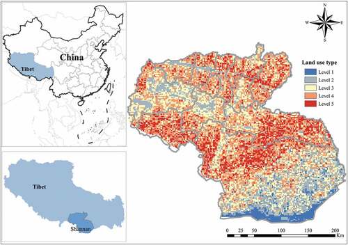
The ecosystems of Shannan are significant to maintain local and national ecological security (Christopher et al. 2017; Jiang et al. 2021), and they are dominated by forests in southern Shannan, while others are mainly alpine scrubland and meadow with obvious horizontal and vertical differentiation. Water resources are very rich with average 70.6 billion cubic meters (m³) for the annual runoff of rivers (average flow rate 937 m³/s) within the administrative boundary, which are concentrated in Brahmaputra River basin located in northern Shannan (Tang 2014; Liu 2008; Jiang et al. 2021).

Data collection

The time-series data of land use (1990, 1995, 2000, 2005, 2010, and 2015), as well as the corresponding normalized difference vegetation index (NDVI) and digital elevation model (DEM), were collected from the Data Center for Resources and Environmental Sciences (The Chinese Academy of Sciences, Beijing, China) (http://www.resdc.cn/). The spatial resolution of them is 1 km. Besides, the elevation data with 30 m spatial resolution is acquired from the Geospatial Data Cloud (The Chinese Academy of Sciences, Beijing, China) (http://www.gscloud.cn/). Socio-economic data, including population and GDP, are retrieved from Tibet statistical yearbooks (Tibet Autonomous Region Bureau of Statistics, 1991–2021). In this study, the ESH and urbanization degree in Shannan were calculated based on a 2-km grid (Tong et al. 2004; Wang et al. 2012). Spatial data processing was handled using “ArcGIS” (version 10.4) and “Fragstats” (version 4.2) software, and the spatial correlation analysis was conducted by GeoDa software.

Approaches

TG classification

The terrain niche index (TNI) can describe the topographic conditions such as elevation and slope comprehensively and is generally adopted to compare the land-use structure with ESH values. By means of Jenks natural break method (Jenks 1967), the TNI in each grid was grouped into five TGs, including level 1 (0–0.5965), level 2 (0.5965–1.0638), level 3 (1.0638–1.3819), level 4 (1.3819–1.7000), and level 5 (1.7000–2.5352). The terrain niche index formula is shown as follows (Gong et al. 2017):

(1) $T=ln\left[\left(\frac{A}{A_0}+1\right)\times \left(\frac{S}{S_0}+1\right)\right]$(1)

where $T$ represents the TNI, $A$ is the point altitude, $S$ is the point slope, $A_0$ refers to the average altitude of the whole study area, and $S_0$ refers to the average slope of the whole study area.

Assessment of ESH

In this study, we assessed the ESH by using VORS model. There are four indicators in ESH assessment: vigor, organization, resilience, and ecosystem services value (Costanza, Norton, and Haskell 1992; Rapport and Maffi 2011; Shi, Han, and Guo 2020). The ESH index formulas are shown as below (Kang et al. 2018):

(2) $EHI=\sqrt{PHI\times ESV}$(2)

(3) $PHI=\sqrt[3]{EV\times EO\times ER}$(3)

where $EHI$ indicates ESH value. $PHI$ and $ESV$ represent ecosystem physical health status and ecosystem services value, respectively. $EV$, $EO$, and $ER$ correspondingly mean ecosystem vigor, ecosystem organization, and ecosystem resilience. To reduce various index dimensions, all indexes are standardized from 0 to 1. The natural break point approach in GIS was applied to classify five levels of ESH based on the 1990 baseline: degraded, unhealthy, average health (ave-health), suboptimal health (sub-health), and highest health (Shi, Han, and Guo 2020).

In general, the primary productivity, metabolic capacity,and activity capacity of the ecosystem are manifested through natural ecosystem vigor (Phillips, Hansen, and Flather 2008). In this study, NDVI was selected for assessing ecosystem vigor on the basis of land-use types because it is closely related to primary productivity (Cui, Ren, and Sun 2015; He et al. 2019). The structural ecosystem stability is represented by organizational factors covering spatial heterogeneity, landscape connectivity, and landscape morphology (Xiao et al. 2019). Referring to interrelated literature, we adopted the index equation of ecosystem organization (He et al. 2019) outlined as follows:

(4) $EO=0.35LH+0.35LC+0.30IC$(4)

where $EO$ presents ecosystem organization. $LH$ and $LC$ denote landscape heterogeneity and landscape connectivity. $IC$ indicates the path connectivity index of the main ecosystem including forest, grass, and wetland.

Facing external distractions, the resilience function of ecosystem can contribute to the stability of structure and pattern (Costanza 2012). To measure the ecosystem resilience, the sum of the area-weighted ecosystem resilience coefficients concerning each land-use type is applied (He et al. 2019), and the calculation formula of ecosystem resilience index is outlined as follows:

(5) $ER=\sum _{i=1}^{n}L{A}_i\times ER{C}_i$(5)

where $ER$ denotes ecosystem resilience. $L{A}_i$ refers to the area of land-use type i with $ER{C}_i$ referring to the ecosystem resilience coefficient of land-use type i conducted by He et al. (2019). n is the number of land-use types.

On the strength of measurement model put forward by Costanza et al. (1997), Xie et al. (2008) suggested that the value per unit area of ecosystem services in China can be applied to evaluate the regional ecosystem services value. Therefore, this method is used to calculate ESV combined with the area of different land-use types in Shannan as follows:

(6) $ESV=\sum _{i=1}^{n}L{A}_i\times P_i$(6)

where $ESV$ represents the total values of ecosystem services per unit with $P_i$ referring to the values per unit area of i conducted by Xie et al. (2008).

Assessment of urbanization

Usually, economic development, population growth, urban land expansion, and social life shifting were used to evaluate the impacts of urbanization (Bai, Shi, and Liu 2014). Population growth and economic development have laid the foundation for urbanization. Changes in lifestyle and the expansion of urban land indicate the social and spatial signs of urbanization, respectively (Peng et al. 2017). As it is difficult to spatialize social data, we have selected indicators to characterize urbanization in terms of economic development, population growth, and land expansion. Specifically, we use GDP density (GDPD) and population density (PD) to quantify economic and population urbanization, and the urban land percentage (ULP) is applied for indicating land urbanization. Due to the high overlapping of the spatial distributions of PD, GDPD, and ULP, these indicators can be integrated into a comprehensive indicator named as comprehensive urbanization level (CUL). The CUL value is identified based on the average value of the above indicators that are ranging between 0 and 1 through range standardization. The range standardization formula is shown as follows:

(7) $U_{i,j}^{\prime }=\frac{U_{i,j}-U_{i,min}}{U_{i,max}-U_{i,min}}$(7)

where $U_{i,j}^{\prime }$ refers to the standardized value of $U_{i,j}$, which is the original value of the $i^{th}$ urbanization indicator (i.e., PD, GDPD, or ULP) in the $j^{th}$ grid. $U_{i,max}$ and $U_{i,min}$ are the maximum and minimum values of the $i^{th}$ urbanization indicator across all grids, respectively.

Spatial correlation analysis between urbanization and ESH

In this study, we attempted to assess the spatial relationship between urbanization and ESH based on global and local bivariate Moran’s I index; the former shows the level of spatial correlation between urbanization and ESH that proposed by Moran (1950), and the latter presents the spatial similarity of the different spatial units (Shi, Han, and Guo 2020). The formulas are shown as follows:

(8) $I=\frac{N{\sum }_i^N{\sum }_{j\ne i}^N{W}_{ij}{Z}_i{Z}_j}{\left(N-1\right){\sum }_i^N{\sum }_{j\ne i}^N{W}_{ij}}$(8)

(9) $I_{kl}^i=\frac{X_k^i-{\bar{X}}_k}{{\sigma }_k}\sum _{j=1}^N{W}_{ij}\frac{X_l^j-{\bar{X}}_l}{{\sigma }_l}\hspace{0.17em}$(9)

where $I$ and $I_{kl}^i$ are the global and local bivariate Moran’s I for ESH and urbanization, respectively. $N$ represents the spatial units number, $W_{ij}$ is spatial weight matrix for measuring spatial correlation between the adjacent spatial unit $i$ and $j$ (Amaral and Anselin 2014), $X_k^i$ is the value of attribute $k$ of spatial unit $i$, ${\bar{X}}_k$ is the average attribute $k$, ${\sigma }_k$ is the $k$’s variance, $X_l^j$ is the attribute $l$’s value of spatial unit $j$, ${\bar{X}}_l$ is the average attribute $l$, and ${\sigma }_l$ is the $l$’s variance.

The spatial agglomeration map divided the regions into five types, including not significant, high–high, low–low, low–high, and high–low. Moran’s I > 0 shows that there is a positive correlation between ESH and urbanization, while Moran’s I < 0 indicates that there is a negative correlation between the two. Monte Carlo simulation test was carried out for data test, and the random simulation times were set to 9999 times (randomization = 9999). To verify the modeling results for spatial correlation between ESV and urbanization, the statistically significant value at 0.1% level is considered as credible results.

Results

Land-use changing based on different TGs

The differences in distribution of various land-use type changing were found on different levels of TGs (Figure 2 and 3). From 1990 to 2015, the area proportions of farm land and forest land decreased with TG increasing, and those of grassland remained stable across the period mainly concentrated on the TGs of levels 3 and 4. The wetland area changed with fluctuation, which was significantly observed on level 2 TG. The area proportions of buildup land presented an increase on the TGs of levels 2 and 3 since 2000, and they were hardly found on the TGs of levels 1, 4, and 5, which is not suitable to promote urbanization in this plateau region. The percentage of unused land remained stable across the period on all TGs and presented growing with the rising of TGs, reaching the bottom on the level 2 TG centralized by intense human activities. One-way ANOVA further demonstrated that TGs influence the change in different land-use types, including farm land (p < 0.05), forest land (p < 0.01), buildup land (p < 0.01), and unused land (p < 0.05). However, TGs did not always determine the differences in grass land and wetland changing during 1990–2015. The area proportions of forest land were significantly larger than others on all TGs.

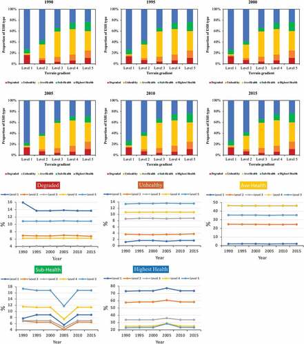
Figure 2. Area proportions of different ESH levels across 1990–2015 in Shannan based on TGs.

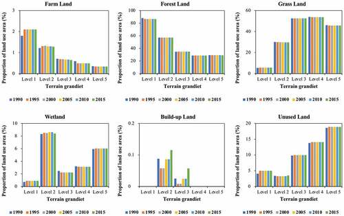
Figure 3. Area proportions of land-use types in Shannan based on TGs.

Spatial variation of ESH based on different TGs

Jenks natural break method is used hereby to divide the ESH into five classes: degraded (0–0.11), unhealthy (0.11–0.32), ave-health (0.32–0.49), sub-health (0.49–0.62), and highest health (0.62–0.78). The ESH distribution and their changes with different TGs during 1990–2015 (Figure 3) indicate that the ecosystems of Shannan were overall in ave-health and highest health levels with slight interannual variations. During the study period, the area proportion of the highest health level increased by 1.98% (level 5 TG), 1.07% (level 2 TG), 0.68% (level 1 TG), and 0.56% (level 4 TG), respectively. Meanwhile, those of degraded level increased by 2.85% at the level 3 TG but significantly decreased by 14.11% at the level 1 TG and 2.69% at the level 2 TG, respectively, which mainly happened before 2000 due to less human intervention. Considering all TGs, by 2015, the area proportion at the highest health level increased by 0.68% and those of degraded level decreased by 1.51%, indicating overall ESH improvements occurred in Shannan, which may benefit from a series of ecological projects including afforestation, returning farmland to forests, and wetland protection (Bai et al. 2015).

From the perspectives of spatial heterogeneity, significant differences were found in ESH at different TGs. The areas of highest health decreased and those of sub-health increased with TG rising. Meanwhile, the areas of unhealthy and degraded increased with TGs rising from levels 2 to 5. The changes in different TGs with five ESH levels presented that areas with lower TGs (level 1 and level 2) achieved healthier levels of ESH. From 1990 to 2015, the area with a highest health on the level 1 TG averagely accounted for 74% of the whole region. Therefore, we speculate that ecosystems are relatively healthy at lower TGs in Shannan, and ESH would be weakened with TG rising due to less vegetation coverage and worse green patch connectivity. Area of ave-health occupied higher land proportion at TGs with level 3 (47%), level 4 (47%), and level 5 (35%), respectively. Notably, the percentages of areas with a degraded level present more than 11% at both highest and lowest TGs by 2015, indicating that TGs have less impacts on worst ESH distribution in these regions. In terms of ESH changing at the same TG, the area with degraded level on the level 3 TG increased by 2.85%, while the areas with highest health and sub-health decreased by 0.20% from 1990 to 2015. This result suggests that rapid land urbanization happened in the level 3 TG (Figure 2) leads to the declines in ESH during the study period, responding to the negative impacts of urbanization on ESH (Wang et al. 2021; Chen et al. 2022).

Spatial correlation between urbanization and ESH

The spatial global and local correlation analysis for the two variables of ESH and CUL was conducted to evaluate the response of ESH to urbanization. Figure 4 and Table 1 show the spatial relationship between urbanization (indicated by CUL) and ESH. The global bivariate Moran’s I in Shannan are −0.237 for 1990, −0.187 for 1995, −0.172 for 2000, −0.167 for 2005, −0.142 for 2010, and −0.176 for 2015. For Shannan Prefecture, the results show that urbanization and ESH were negatively related, and these negative correlations tended to shrink since 1995. The local spatial correlation analysis results are shown in Figure 5. The number of grids for high ESH–low CUL type occupies the largest proportion among the grids, indicating the agglomeration impacts. Besides, the effect of high ESH–low CUL type clustering is more significant at lower TGs in southern Shannan covered by natural forest, and this type aggregates mainly located on the lower TGs. For the low ESH–high CUL type, it is obviously concentrated in the northern Shannan where dense population is concentrated. Therefore, the relatively high level of urbanization in these areas results in a low level of ESH.

Figure 4. Moran’s I index of ESH and urbanization in Shannan from 1990 to 2015 (the slope of lines indicate the negatives of Moran’s I scores).

Figure 5. Spatial aggregation of ESH and urbanization in Shannan from 1990 to 2015.

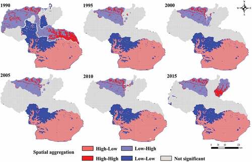
Table 1. Moran’s I index of ESH and urbanization with the significant level in Shannan from 1990 to 2015.

Index	1990	1995	2000	2005	2010	2015
I	−0.237	−0.187	−0.172	−0.167	−0.142	−0.176
P	<0.001	<0.001	<0.001	<0.001	<0.001	<0.001
Z	−89.5221	−70.6749	−64.4299	−62.2058	−52.8158	−64.8089

The value I is Moran’s index; the p (p-value) is the probability, which represents an event happening probability. p < 0.01 showed a statistically significant difference and P < 0.001 showed a more statistically significant difference. Z-score is a multiple of the standard deviation that represents the data dispersion or aggregation, |Z| > 2.58, corresponding to p < 0.01, showing a statistically significantdifference.

Discussion

Relationships between TG, land use, and ESH

Topography is a significant factor that affects land use, ecosystem services, and ESH (Xu et al. 2019; Shi, Han, and Guo 2020; Zhao et al. 2021). Through the investigation focusing on different land-use types on all levels of TGs, we found that land-use types in Shannan are mainly forest land and grass land, the distribution of which varies significantly on different TGs. The area of farm land decreases with the increase in the TGs, probably due to higher elevation and slope restricting development of agriculture (Shi, Han, and Guo 2020). The decreases in forest area are found with TG increasing, which is different from the previous study concerning low-altitude regions, including Anhui province, Gannan region in Jiangxi province, and Huailai County in Hebei province (Ha, Ding, and Men 2015; Wu, Wang, and Tan 2016; Shi, Han, and Guo 2020). In the case of Gannan region located in Southeast China, cities are generally located on the TGs of lower levels where the higher degree of human interference frequently occurs. The forests are logged and exploited for further urbanization in these lower TG regions, while those will be conserved at higher TG regions with less human interference, indicating that the topography reduces the external stressors for ESH (Shi, Han, and Guo 2020). Different from synergistic effects between better ESH and higher TGs observed outside Tibet Plateau, the distribution of forest in Shannan is mainly affected by hydrothermal conditions, which turn worse for plant growth (lower temperature, less moisture, soil depletion, etc.) with TG rising. Therefore, less forest could be found in higher TG, and they mainly located on lower TGs, especially the level 1 TG, supporting better ESH maintenance on lower TGs in this plateau region. Meanwhile, both the increasing areas of grass land and unused land are found on higher TGs, which are not suitable for farming and urban sprawl. Because of lower hydrothermal condition required by grass growth, the grass land can still spread naturally in these regions. Notedly, buildup land is mainly distributed on the TGs of levels 2 and 3, and the development mode of which is in line with local actual situation influenced by climatic and topographic features of plateau.

From the perspective of different TGs, the ESH of Shannan is overall in good health, but the situations on different TGs are quite different. Averagely, at the TG of level 1, the highest health level of ESH (mainly contributed by virgin forest) occupied 74% and that with degraded level (mainly contributed by farmland) occupied 14%. At the TG of level 2, the ESH mainly includes the highest and ave-health levels, which presents that ESH still not be significantly disturbed by human intervention. However, at the level 3 TG with rapid urbanization since 2010, the areas of highest health, sub-health, and ave-health levels decreased, while the areas of degraded and unhealthy levels increased, indicating a severe competition between the ecological protection and urbanization. The areas with ave-health ESH mainly were found on the level 4 and 5 TGs, which shows great potential for further ESH improvements or deteriorations on the higher TGs of Shannan. This illustrates that worse ESH potentially would be found at the areas with higher TGs, even without higher degree of human interference.

Relationships between ESH and urbanization

Through investigating the responses of ESH to plateau urbanization, we found that ESH is negatively related to urbanization, which is consistent with previous research (Mitchell et al. 2015; Shi, Han, and Guo 2020). For Shannan Prefecture, the strong high ESH–low CUL agglomeration aggregation type is distributed in southern Shannan on lower TGs, where the national ecosystem function zones for biodiversity conservation located with wide distribution of virgin forests (Christopher et al. 2017). The ESH for these areas was strengthened gradually because of better geomorphic and climatic condition for virgin forest development and the political intervention for construction activity restrictions. However, it still faces up to the challenges of cultivated land reclamation for agriculture (Figure 2). Meanwhile, the significant aggregation type of low ESH–high CUL agglomeration is found in the river valley area of north Shannan covered by a relatively intense population. Although the average TG of this region (2 –4 levels) is not so ideal for urban sprawl in plateau region, the regional urbanization is significant attributed by adequate water supplies, and thereby, the ESH here will be continuously threatened by intense human interference with urbanization. Undeniably, urbanization has played an important role in poverty alleviation and rural revitalization of Shannan, but the urbanization rate of this region still remains a lower level, compared to other prefecture cities outside Tibet plateau. As the water supplies by Brahmaputra River decreased overall in Shannan regions (Xiao et al. 2021), the water resource utilization pressure will be strengthened droved by urbanization, posting challenges to ecological and environmental protection in this ecological fragile areas.

Normally, urbanization will have a significant negative impact on ESH (Wang, Ma, and Zhao 2014), and we have reached similar conclusion in Tibet where the initial urbanization is developing. Although the ESH for Shannan Prefecture has been overall improved from 1990 to 2015, in the future, the ESH still will be threatened by the prospective urbanization process. With geographical and environmental conditions of alpine plateau, the suitable land space for developing urbanization in Shannan is limited. Therefore, land-use exploiting is the most direct approach to promote urbanization and thereby affect ESH (Gordon et al. 2009; Shi, Han, and Guo 2020). Compared to the areas with lower average elevation outside Tibet plateau, higher topography can reduce the external stressors from human interference to better maintain ESH (Shi, Han, and Guo 2020). However, the high topography cannot fully limit the urban sprawl in Shannan since the water supply is the key factor to influence human settlement for urbanization in this water-shortage and alpine region. The areas with higher TGs still will be threatened by the urban sprawl if more buildup land is required to promote urbanization, and this challenge should be well addressed by future land policies.

Located on the national border, the sustainable development of Shannan plays a key role in maintaining ecological security of Qinghai-Tibet Plateau and even China since Shannan is highly susceptible to ecological vulnerability due to its typical alpine climate and topography (Jiang et al. 2021). Therefore, it is essential to fully balance the relationship between protection and development toward green development based on local actual situation in Qinghai-Tibet Plateau. For example, the future land policies of Shannan Prefecture can vigorously focus on covering ecological product realization (e.g., ecotourism) based on rich forest resources on the lower TGs and explore an effective path to transform the natural endowment into economic benefit for indigenous inhabitants, aiming at restraining the expansion of agricultural land for maintaining better ESH and ecosystem service supply (Mandle et al. 2019). Meanwhile, the developments of wastewater treatment facilities to collect wastewater for water resource recycling are urgently needed in the river valley area experiencing rapid urbanization, alleviating water shortage and pollution. Moreover, the wide distribution of grass land and unused land on level 3–5 TGs in central Shannan can be officially planned to provide available spaces for promoting livestock husbandry and artificial afforestation programs (Jiang et al. 2021), which contribute to establishing a “Tibet-Style” development pathways instead of forming the hinterland of industrialization that attracts immigration of more industrial factories outside Tibet. These measures can provide a digital scientific foundation for land planning toward green development in Shannan Prefecture, as well as other regions in Tibet.

There still exist some inevitable limitations in this study. The impact of urbanization on ESH was assessed merely by spatial and statistical data, and more local surveys needed to be carried out to acquire first-hand data reflecting people’s livelihood, aiming at minimizing the bias that green development depending more on ESH than urbanization, since economic development and poverty elimination drove by urbanization are political priorities addressed by “13^th Five-Year Plan” of Shannan since 2016 (The People’s Government of Shannan 2016). Drove by “China Western Development Strategy” and “Promoting Urbanization Strategy” (NPC (The National People’s Congress of the People’s Republic of China) 2013; Xian et al. 2019), the impacts of urbanization on Tibet’s ESH will remain in a long time. In future, based on VORS model, further studies concerning entire Tibet urbanization beyond Shannan are needed to assess the responses of plateaus’ ESH to urbanization.

Conclusions

ESH varies greatly both temporally and spatially influenced by natural landscape configuration and anthropogenic interference. In this study, we adopt VORS model to investigate the relationships between ESH and urbanization in a plateau-type region with ecological fragility. We found that topography is the fundamental factor to affect the land-use types and then ESH, which mainly reach the average health and highest health levels during 1990–2015. By 2015, the area proportion at the highest health level increased by 0.68%, while that of degraded level decreased by 1.51%. Our results also echo the findings of other studies in terms of the higher terrain gradients (TGs), reducing the external anthropogenic stressors for ESH, but addressing the worse ESH could also be found on higher TGs without significant human interference in the plateau region, revealing the differences in the responses of ESH to urbanization for the Tibet and outside Tibet. Through spatial correlation analysis, we found that urbanization had a negative impact on ESH, especially the areas on middle TGs with the dense population, but this negative effect presented slightly decreased from 1990 to 2015. The better ESH could be found on lowest TGs, which is the basis for local policy formulation to explore a green development pathway. The result showed the law of temporal-spatial ESH changing in Shannan and provided information for rationally organizing future urbanization process based on reasonable land policies, which could be taken to improve ESH on different TGs according to the actual plateau situation of the Tibet, aiming at advancing people livelihood improvement from the perspectives of economic development and ecological conservation.

Acknowledgments

This research was funded by the Second Tibetan Plateau Scientific Expedition and Research (No.2019QZKK0308) and the National Natural Science Foundation of China (No. 42101290). The authors would like to thank the editors and anonymous reviews for their helpful comments.

Disclosure statement

No potential conflict of interest was reported by the authors.

Correction Statement

This article has been corrected with minor changes. These changes do not impact the academic content of the article.

Additional information

Funding

This work was supported by Second Tibetan Plateau Scientific Expedition and Research (No.2019QZKK0308) and National Natural Science Foundation of China (No. 42101290).

References

- Amaral, P. V., and L. Anselin. 2014. “Finite Sample Properties of Moran’s—Test for Spatial Autocorrelation in Tobit Models[J].” Papers in Regional Science 93: 1–12. doi:10.1111/pirs.12034.
- Bai, X., P. Shi, and Y. Liu. 2014. “Society: Realizing China’s Urban dream[J].” Nature 509 (7499): 158–160. doi:10.1038/509158a.
- Bai, S. Y., Q. Wu, J. Q. Shi, and Y. Lu. 2015. “Analysis on Vegetation Coverage Change in Shannan, Tibet, China Based on Remotely Sensed data[J].” Journal of Desert Research 35 (5): 1396–1402.
- Cao, C., and X. Li. 2018. “Health Assessment of River Ecosystem at the District and County Scales: A Case Study of Fangshan District in Beijing[J].” Acta Ecologia Sinica 38: 4296–4306.
- Chen, W. X., X. L. Zhao, M. X. Zhong, J. F. Li, and J. Zeng. 2022. “Spatiotemporal Evolution Patterns of Ecosystem Health in the Middle Reaches of the Yangtze River Urban Agglomerations[J].” Acta Ecologica Sinica 42 (1): 138–149.
- Christopher, N. J., B. Andrew, W. B. Barry, C. B. Jessie, G. Mauro, G. C. Lei, and M. W. Janet. 2017. “Biodiversity Losses and Conservation Responses in the Anthropocene[J].” Science 356 (6335): 270–275. doi:10.1126/science.aam9317.
- Costanza, R., B. G. Norton, and B. D. Haskell. 1992. Ecosystem Health: New Goals for Environmental Management[M]. Washington: Island Press.
- Costanza, R., R. D’Arge, R. De Groot, S. Farber, M. Grasso, B. Hannon, K. Limburg, S. Naeem, R. V. O’Neill, and J. Paruelo. 1997. “The Value of the World’s Ecosystem Services and Natural Capital[J].” Nature 387: 253–260. doi:10.1038/387253a0.
- Costanza, R. 2012. “Ecosystem Health and Ecological Engineering[J].” Ecological Engineering 45: 24–29. doi:10.1016/j.ecoleng.2012.03.023.
- Cui, E., L. Ren, and H. Sun. 2015. “Evaluation of Variations and Affecting Factors of Eco-environmental Quality during Urbanization[J].” Environmental Science and Pollution Research 22 (5): 3958–3968. doi:10.1007/s11356-014-3779-6.
- Fayiah, M., S. Dong, S. W. Khomera, S. A. Ur Rehman, M. Yang, and J. Xiao. 2020. “Status and Challenges of Qinghai—Tibet Plateau’s Grasslands: An Analysis of Causes, Mitigation Measures, and Way Forward[J].” Sustainability 12 (3): 1099. doi:10.3390/su12031099.
- Fu, A., Y. Chen, and W. Li. 2009. “Ecosystem Health Assessment in the Tarim River Basin by Using Analytical Hierarchy Process[J].” Resource Science 31 (9): 1535–1544.
- Gong, W., H. Wang, X. Wang, W. Fan, and P. Stott. 2017. “Effect of Terrain on Landscape Patterns and Ecological Effects by a Gradient-based RS and GIS Analysis[J].” Journal of Forestry Research 28 (5): 1061–1072. doi:10.1007/s11676-017-0385-8.
- Gordon, A., D. Simondson, M. White, A. Moilanen, and S. A. Bekessy. 2009. “Integrating Conservation Planning and Land Use Planning in Urban Landscapes[J].” Landscape and Urban Planning 91 (4): 183–194. doi:10.1016/j.landurbplan.2008.12.011.
- Ha, K., Q. L. Ding, and M. X. Men. 2015. “Spatial Distribution of Land Use and Its Relationship with Terrain Factors in Hilly Area[J].” Geographical Research 34 (5): 909–921.
- Han, Y., D. Yu, and K. Chen. 2021. “Evolution and Prediction of Landscape Patterns in the Qinghai Lake Basin[J].” Land 10 (9): 921. doi:10.3390/land10090921.
- He, J., Z. Pan, D. Liu, and X. Guo. 2019. “Exploring the Regional Differences of Ecosystem Health and Its Driving Factors in China[J].” Science of the Total Environment 673: 553–564. doi:10.1016/j.scitotenv.2019.03.465.
- Hou, Y., S. Zhou, B. Burkhard, and F. Müller. 2014. “Socioeconomic Influences on Biodiversity, Ecosystem Services and Human Well-being: A Quantitative Application of the DPSIR Model in Jiangsu, China[J].” Science of the Total Environment 490: 1012–1028. doi:10.1016/j.scitotenv.2014.05.071.
- Jenks, G. F. 1967. “The Data Model Concept in Statistical mapping[J].” International Yearbook of Cartography 7: 186–190.
- Jiang, X. Y., R. Li, Y. Shi, and L. Guo. 2021. “Natural and Political Determinants of Ecological Vulnerability in the Qinghai–Tibet Plateau: A Case Study of Shannan, China[J].” ISPRS International Journal of Geo-Information 10 (5): 327. doi:10.3390/ijgi10050327.
- Kang, P., W. P. Chen, Y. Hou, and Y. Z. Li. 2018. “Linking Ecosystem Services and Ecosystem Health to Ecological Risk Assessment: A Case Study of the Beijing-Tianjin-Hebei Urban Agglomeration[J].” Science of the Total Environment 636: 1442–1454. doi:10.1016/j.scitotenv.2018.04.427.
- Kim, Y.-O., and F.-L. Xu. 2014. “Marine Ecosystem Health Assessments in Korean Coastal Waters[J].” Ocean Science Journal 49 (3): 249–250. doi:10.1007/s12601-014-0025-6.
- Li, C. Y., H. L. Qin, and W. S. Gao. 2006. “Ecosystem Health Evaluation in Ecotone between Agriculture and Animal Husbandry in Northern China Farmland: The Case of Wu Chuan County[J].” Chinese Agricultural Science Bulletin 22 (2): 347–350.
- Li, W., Y. Wang, S. Xie, and X. Cheng. 2021. “Coupling Coordination Analysis and Spatiotemporal Heterogeneity between Urbanization and Ecosystem Health in Chongqing Municipality, China[J].” Science of the Total Environment 791: 148311. doi:10.1016/j.scitotenv.2021.148311.
- Liu, X. 2008. Study on Urbanization Path and Development of Small Towns in Less Developed Areas of Western China[M]. Beijing: Ethnic Publishing House.
- Lv, Y. L., R. S. Wang, Y. Q. Zhang, H. Q. Su, P. Wang, A. Jenkins, R. C. Ferrier, M. Bailey, and G. Squire. 2015. “Ecosystem Health Towards sustainability[J].” Ecosystem Health and Sustainability 1: 1–15.
- Mandle, L., Z. Y. Ouyang, J. Salzman, and C. Gretchen. 2019. “Green Growth that Works: Natural Capital Policy and Finance Mechanisms around the World[M].” Washington DC: Island Press.
- Mitchell, M. G. E., A. F. Suarez-Castro, M. Martinez-Harms, M. Maron, C. McAlpine, K. J. Gaston, K. Johansen, and J. R. Rhodes. 2015. “Reframing Landscape Fragmentation’s Effects on Ecosystem Services[J].” Trends in Ecology & Evolution 30 (4): 190–198. doi:10.1016/j.tree.2015.01.011.
- Moran, P. 1950. “Notes on Continuous Stochastic Phenomena[j].” Biometrika 37: 17–23. doi:10.1093/biomet/37.1-2.17.
- NPC (The National People’s Congress of the People’s Republic of China). 2013. “The State Council’s Reports for the Implementation of ‘China Western Development Strategy’ [EB/OL].” http://www.npc.gov.cn/npc/zxbg/gwygyssxbdkfzlqkdbg/2013-10/22/content1811909.htm, Accessed 13 May 2018).
- Ouyang, X., X. Zhu, and Q. Y. He. 2020. “Incorporating Ecosystem Services with Ecosystem Health for Ecological Risk Assessment: Case Study in Changsha-Zhuzhou-Xiangtan Urban Agglomeration, China[J].” Acta Ecologia Sinica 40 (16): 5478–5489.
- Peng, J., Y. Liu, J. Wu, H. Lv, and X. Hu. 2015. “Linking Ecosystem Services and Landscape Patterns to Assess Urban Ecosystem Health: A Case Study in Shenzhen City, China[J].” Landscape and Urban Planning 143: 56–68. doi:10.1016/j.landurbplan.2015.06.007.
- Peng, J., L. Tian, Y. Liu, M. Zhao, Y. Hu, and J. Wu. 2017. “Ecosystem Services Response to Urbanization in Metropolitan Areas: Thresholds Identification[J].” Science of the Total Environment 607: 706–714. doi:10.1016/j.scitotenv.2017.06.218.
- The People’s Government of Shannan. 2016. “Outline of the 13th Five-Year Plan for National Economic and Social Development of Shannan, Tibet Autonomous Region[EB/OL].” http://www.shannan.gov.cn/zwgk/zfxxgkml/201905/P020190513366712390803.pdf, Accessed date 1 December 2021
- Phillips, L. B., A. J. Hansen, and C. H. Flather. 2008. “Evaluating the Species Energy Relationship with the Newest Measures of Ecosystem Energy: NDVI versus MODIS Primary Production[J].” Remote Sensing of Environment 112 (12): 4381–4392. doi:10.1016/j.rse.2008.08.002.
- Rapport, D. J., R. Costanza, and A. J. McMichael. 1998. “Assessing Ecosystem Health[J].” Trends in Ecology & Evolution 13 (10): 397–402. doi:10.1016/S0169-5347(98)01449-9.
- Rapport, D. J., and L. Maffi. 2011. “Eco-cultural Health, Global Health, and Sustainability[J].” Ecological Research 26 (6): 1039–1049. doi:10.1007/s11284-010-0703-5.
- Shannan Municipal Statistics Bureau. 2021. “Statistical Bulletin of National Economic and Social Development of Shannan Prefecture in 2020[EB/OL].” http://www.shannan.gov.cn/zwgk/zfxxgkml/202105/t20210525_82080.html, Accessed 13 November 2021)
- Shen, W., Z. Zheng, L. Pan, Y. Qin, and Y. Li. 2020. “A Integrated Method for Assessing the Urban Ecosystem Health of Rapid Urbanized Area in China Based on SFPHD Framework[J].” Ecological Indicators 121: 107071. doi:10.1016/j.ecolind.2020.107071.
- Shi, Y., R. Han, and L. Guo. 2020. “Temporal–spatial Distribution of Ecosystem Health and Its Response to Human Interference Based on Different Terrain Gradients: A Case Study in Gannan, China[J].” Sustainability 12 (5): 1773. doi:10.3390/su12051773.
- Su, M., B. D. Fath, and Z. Yang. 2010. “Urban Ecosystem Health Assessment: A review[J].” Science of the Total Environment 408 (12): 2425–2434. doi:10.1016/j.scitotenv.2010.03.009.
- Sun, T., W. Lin, G. Chen, P. Guo, and Y. Zeng. 2016. “Wetland Ecosystem Health Assessment through Integrating Remote Sensing and Inventory Data with an Assessment Model for the Hangzhou Bay, China[J].” Science of the Total Environment 566: 627–640. doi:10.1016/j.scitotenv.2016.05.028.
- Tang, L. L. 2014. “The Study of the Construction of Ecological Civilization Demonstration Zone in Lhoka, Tibet[D]”. Ph.D. Dissertation, Nanjing Agricultural University, Nanjing, China.
- Tibet Autonomous Region Bureau of Statistics. 1991-2021. Tibet Statistical Yearbook 1991-2021[M]. Beijing: China Statistics Press.
- Tong, C., J. Wu, S. Yong, J. Yang, and W. Yong. 2004. “A Landscape-scale Assessment of Steppe Degradation in the Xilin River Basin, Inner Mongolia, China[J].” Journal of Arid Environments 59 (1): 133–149. doi:10.1016/j.jaridenv.2004.01.004.
- Wang, D. G., B. Q. Hu, Y. X. Rao, and W. H. Li. 2012. “Research on Functional Zoning of Karst Land System at County Regional Scale Based on the Methods of Lattice and ANN[J].” Research of Soil and Water Conservation 19 (2): 131–136.
- Wang, S., H. Ma, and Y. Zhao. 2014. “Exploring the Relationship between Urbanization and the Eco-environment—A Case Study of Beijing-Tianjin-Hebei Region[J].” Ecological Indicators 45: 171–183. doi:10.1016/j.ecolind.2014.04.006.
- Wang, Q. S., M. Q. Liu, S. Tian, X. L. Yuan, Q. Ma, and H. L. Hao. 2021. “Evaluation and Improvement Path of Ecosystem Health for Resource-based City: A Case Study in China[J].” Ecological Indicators 128: 107852. doi:10.1016/j.ecolind.2021.107852.
- Wen, Z. Q., X. Li, B. Liu, and T. H. Li. 2021. “A Comprehensive Evaluation Method for Plateau Freshwater Lakes: A Case in the Erhai Lake[J].” Ecosystem Health and Sustainability 7 (1): 1993753. doi:10.1080/20964129.2021.1993753.
- Wu, J., S. Wang, and J. Tan. 2016. “Analysis on Terrain Gradient Effect Based on Land Use Change in Anhui Province[J].” Resources and Environment in the Yangtze Basin 25 (2): 239–248.
- Wu, J. S., D. J. Cheng, Y. Y. Xu, Q. Huang, and Z. Feng. 2021. “Spatial-temporal Change of Ecosystem Health across China: Urbanization Impact Perspective[J].” Journal of Cleaner Production 326: 129393. doi:10.1016/j.jclepro.2021.129393.
- Xian, C., X. Zhang, J. Zhang, Y. Fan, H. Zheng, J. Salzman, and Z. Ouyang. 2019. “Recent Patterns of Anthropogenic Reactive Nitrogen Emissions with Urbanization in China: Dynamics, Major Problems, and Potential Solutions[J].” Science of the Total Environment 656: 1071–1081. doi:10.1016/j.scitotenv.2018.11.352.
- Xiao, R., Y. Liu, X. Fei, W. Yu, Z. Zhang, and Q. Meng. 2019. “Ecosystem Health Assessment: A Comprehensive and Detailed Analysis of the Case Study in Coastal Metropolitan Region, Eastern China[J].” Ecological Indicators 98: 363–376. doi:10.1016/j.ecolind.2018.11.010.
- Xiao, Y., Q. Xiong, P. Liang, and Q. Xiao. 2021. “Potential Risk to Water Resources under Eco-restoration Policy and Global Change in the Tibetan Plateau[J].” Environmental Research Letters 16 (9): 094004. doi:10.1088/1748-9326/ac1819.
- Xie, G. D., L. Zhen, C. X. Lu, Y. Xiao, and C. Chen. 2008. “Expert Knowledge Based Valuation Method of Ecosystem Services in China[J].” Journal of Natural Resources 23 (5): 911–919.
- Xu, N. Y., S. Q. Sun, D. Y. Xue, and L. Guo. 2019. “Ecosystem Service Value and Its Spatial Response to Human Interference on the Basis of Terrain Gradient in Gannan Region, China[J].” Acta Ecologia Sinica 39 (1): 97–107.
- Zhang, J., L. Guo, C. S. Song, and W. H. Xu. 2021. “Assessment of Ecosystem Assets in Qinghai-Tibet Plateau: A Case Study of Shannan City[J].” Acta Ecologia Sinica 41 (22): 9095–9102.
- Zhao, Y. T., W. L. Li, D. Chen, C. Yu, X. L. Zhao, J. Xu, and X. L. Guo. 2017. “Dynamic Assessment of Alpine Pasture Grassland Ecosystem health—A Case Study from the Gannan Region[J].” Pratacultural Science 34 (1): 16–29.
- Zhao, Y., R. Han, N. Cui, J. Yang, and L. Guo. 2021. “The Impact of Urbanization on Ecosystem Health in Typical Karst Areas: A Case Study of Liupanshui City, China[J].” International Journal of Environmental Research and Public Health 18 (1): 93. doi:10.3390/ijerph18010093.