Tectonic discrimination of olivine in basalt using data mining techniques based on major elements: a comparative study from multiple perspectives

ABSTRACT

The olivine in basalt records much information about formation and evolution of basaltic magma, which may help to discriminate basalt tectonic settings. However, the viewpoint that olivine is connected with the tectonic setting where it formed is controversial. To verify the hypothesis, we intend to discriminate the basalt tectonic settings by geochemical characteristics of olivine. The data mining technique is selected as an effective tool for this study, which is a new attempt in geochemical research. The geochemical data of olivine used is extracted from open-access and comprehensive petrological databases. The classification performance of Logistic regression classifier, Naïve Bayes, Random Forest and Multi-layer perception (MLP) algorithms is firstly compared under some constraints. The results of the basic experiment indicate that MLP has the highest classification accuracy of about 88% based on raw data, followed by Random Forest. But this does not fully prove the hypothesis is credible. Then, the cross-validation method and other measurement criteria are integrated for scientific and in-depth comparative analysis. The advanced experiments mainly include the comparison of different data preprocessing methods, combinations of geochemical characteristics and sample data volumes. It turns out that chemical composition of olivine in basalt has the function of discriminating tectonic settings.

KEYWORDS:

• Olivine in basalt
• tectonic setting
• geochemical discrimination
• data mining
• comparative study

1. Introduction

Olivine is one of the most common minerals on earth, which is the main mineral composition of mantle rock, and one of the earliest minerals formed when magma crystallizes (Zhou, Chen, & Chen, 1980). Olivine is also a major rock-forming mineral in basic and ultrabasic igneous rocks, such as basalt, gabbro and peridotite. Olivine mainly composes of Mg or Fe and contains other elements, such as Mn, Ni and Co, whose crystals are granular and dispersed in rocks or granular aggregates (Enciso-Maldonado et al., 2015). As we all know, the basalt and its minerals have always been the main means to explore the magmatic process, the hot state of the mantle and the composition of the mantle elements (Di et al., 2017). As the most important mineral composition of mantle rock and the earliest crystalline mineral of magma, the basic elements of olivine in basalt can provide effective information about the partial melting of mantle, early crystallization process of magma and mantle metasomatism (Howarth & Harris, 2017).

The basalt is usually divided into different types based on the tectonic setting. The mid-ocean ridge basalt (MORB), ocean island basalt (OIB) and island arc basalt (IAB) are the three types of basalt most concerned by the academic community (Vermeesch, 2006). Then, how to discriminate the tectonic settings of basalt has become an important issue in geochemistry. In general, we can discriminate the tectonic settings formed by magmatic rocks, mainly including the basalt and granite, and master the chemical properties of magma sources in terms of the chemical composition of magmatic rocks. This is a common and feasible discrimination approach, which has been proved by many facts (Bhatia & Crook, 1986; Li, Arndt, Tang, & Ripley, 2015; Sánchez-Muñoz et al., 2017). The olivine in basalt records much information about the formation and evolution of basaltic magma, which is helpful to discriminate the three tectonic settings. At present, it is generally believed that the chemical composition of olivine is one piece of important evidence to identify whether basalt is primitive magma, but the viewpoint that olivine is closely related to the tectonic setting where it formed is controversial. The paper aims to prove the rationalization of the latter.

In the 1970s, Pearce and Cann (1973) first proposed the basalt discrimination diagram based on the chemical composition. The basalt discrimination diagram organically combines the tectonic setting with the geochemical characteristics of basalt, thus opening up a new way for the study of plate tectonics and continental orogenic belts. This greatly enriched the research contents of basalt. The basalt discriminant diagrams have been widely used in academic circles due to their solid theoretical foundations and concise forms of expression (Pearce, 1996). The study of basalt tectonic setting has also been pushed to the peak since then. Even now, the discrimination diagram is still the main method for basalt tectonic setting discrimination. However, with the increasing use of the discrimination diagram, its inherent defects gradually appear, such as the empiricism and subjectivity, lack of rigorous theory, contradiction of discrimination and limitation of application (Luo et al., 2018; Zhang, 1990). The drawbacks mentioned above greatly affect the classification accuracy and work reliability of the discrimination diagram. To our knowledge, it is difficult to discriminate the basalt tectonic settings using the discrimination diagram based on the geochemical characteristics of olivine in basalt. And also, there is almost no introduction about the use of olivine in the basalt tectonic setting discrimination in the literatures. Therefore, we need to find another way to discriminate the tectonic settings of basalt on the basis of the chemical composition of olivine.

The data mining technique is a good choice. With the rapid development of new technologies, such as big data and cloud computing, as well as the substantial improvement of the computing capacity of computer hardware, the data mining technique has increasingly aroused great concern among domestic and foreign scholars in recent years (Zhou et al., 2018). In the areas of pattern recognition, function approximation and simulation modeling, fruitful results have been achieved. But now in geochemistry, the research on discriminating the tectonic settings of basalt using data mining is still in the initial stage. Petrelli and Perugini (2016) used Support Vector Machines (SVM) to discriminate the tectonic settings of volcanic rocks and obtained high classification scores. Ueki, Hino, and Kuwatani (2018) adopted SVM, Random Forest and Sparse Multinomial Regression approaches for classification performance comparison. The results indicated that data mining is a highly effective tool in geochemical research. Based on the two successful cases, we intend to employ data mining to do some simulation experiments, which all involves the tectonic setting discrimination of basalt based on the chemical composition of olivine. Being an attempt in geochemical research, we proceed from the perspective of comparative research, which may lay the groundwork for future research (Han, Li, Ren, & Liu, 2018). This just determines that there are some fundamental comparative tests, mainly including the comparison of different data mining algorithms, data preprocessing methods, combinations of geochemical characteristics and sample data volumes. Nevertheless, we have to admit that the experimental results acquired certainly contain some drawbacks and are open to comments and further research.

This paper is organized as follows. In Section 2, an overall research framework of this paper is introduced. Section 3 presents a brief description of different data mining algorithms, followed by a synopsis of the cross-validation method and measurement criteria. The data description, preliminary experiment and benchmark classification effects are provided in Section 4. Section 5 illustrates and discusses the experimental results and analysis for four comparative tests. The concluding remarks and future work are finally mentioned in Section 6.

2. Overall framework

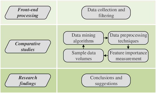
The overall research framework shown in Figure 1 is outlined below.

1. The geochemical data of olivine are collected from the GEOROC and PetDB databases, followed by data cleaning and management, thus laying a good data foundation for this study. It is worth mentioning that the olives data used are measured via common methods of major element analysis, e.g. electron probe microanalysis, EPMA, or instrumental neutron activation analysis, INAA (Arevalo, McDonough, & Luong, 2009).

2. Different data mining algorithms are used to discriminate tectonic settings of the collated olivine in basalt in terms of geochemical characteristics. The classification performance of different data mining algorithms is compared.

3. The effect of data preprocessing on the discrimination results of tectonic settings of olivine has not been considered in the previous step. Hence, the impacts of different data preprocessing techniques on the classification performance of four classifiers are compared.

4. The importance score of each geochemical characteristic of olivine is analyzed through Random Forest. The effects of different combinations of geochemical characteristics on the single and overall classification accuracy of four classifiers are considered. The relationship between the cumulative feature importance and the classification accuracy is also studied.

5. It is necessary to research on the effects of different sample data volumes on the single and overall classification accuracy of four classifiers, when big data mining is used to discriminate tectonic settings of olivine. This will provide a reference for subsequent studies.

6. Four comparative studies are conducted, including the classification performance of four classifiers, the impacts of different data preprocessing techniques, combinations of geochemical characteristics and sample data volumes. Some important conclusions are drawn, and a few valuable suggestions for future research are proposed.

Figure 1. Overall framework diagram.

3. Methodology

3.1. Data mining algorithms

3.1.1. Logistic regression classifier (LRC)

Logistic regression is an approach to learning functions of the form $f:X\to Y$, or $P(Y|X)$ in the case where Y is discrete-valued, and $X=(X_1,X_2,\cdots ,X_n)$ is any vector containing discrete or continuous variables (Mitchell, 2005; Subasi & Ercelebi, 2005). In this section, we will primarily consider the case where Y is a boolean variable, in order to simplify notation. More generally, Y can take on any of the discrete values $\left\{y_1,y_2,\cdots ,y_k\right\}$ which is used in experiments.

Logistic regression assumes a parametric form for the distribution $P(Y|X)$, then directly estimates its parameters from the training data. The parametric model assumed by Logistic regression in the case where Y is boolean as follows

(1) $P(Y=1|X)=\frac{1}{1+exp\left(w_0+{\sum }_{i=1}^n{w}_i{X}_i\right)}$(1)

and

(2) $P(Y=0|X)=\frac{exp\left(w_0+{\sum }_{i=1}^n{w}_i{X}_i\right)}{1+exp\left(w_0+{\sum }_{i=1}^n{w}_i{X}_i\right)}$(2)

Notice that Equation (2) follows directly from Equation (1), because the sum of these two probabilities must equal one.

One highly expedient property of this form for $P(Y|X)$ is that it leads to a simple linear expression for classification. To classify any given X, we generally want to assign the value y_k that maximizes $P(Y=y_k|X)$. In other word, we assign the label $Y=0$ if the following condition holds $\frac{P(Y=0|X)}{P(Y=1|X)}>1$. Substituting from Equations (1) and (2), this becomes $exp\left(w_0+{\sum }_{i=1}^n{w}_i{X}_i\right)>1$.

Then taking the natural log of both sides, we have a linear classification rule that assigns label $Y=0$ if X satisfies $w_0+{\sum }_{i=1}^n{w}_i{X}_i>0$, and assigns $Y=1$ otherwise.

3.1.2. Naïve bayes

Naïve Bayes algorithm is a simple probabilistic classifier based on applying Bayes theorem with naive independence assumptions between the features, which only requires a small number of training data to estimate the parameters necessary for classification (Li, Miao, & Shi, 2014; Ren, Wang, Li, & Han, 2019). Now suppose that a problem instance to be classified, represented by a vector $X=(x_1,x_2,\cdots ,x_n)$, it assigns to this instance probabilities $P(C_k|x_1,x_2,\cdots ,x_n)$ for each of k possible categories. Using Bayes theorem, the conditional probability can be decomposed as

(3) $P(C_k|X)=\frac{P(C_k)P(X|C_k)}{P(X)}$(3)

$P(C_k)P(X|C_k)$ is equivalent to the joint probability model $P(C_k|x_1,x_2,\cdots ,x_n)$because $P(X)$ is constant. Assume that each feature x_i is conditionally independent of every other feature x_j for $j\ne i$, given the category C_k. Thus, the conditional distribution over the class variable C_k is

(4) $P(C_k|x_1,x_2,\cdots ,x_n)=\frac{1}{Z}P(C_k){\prod }_{i=1}^{n}P(x_i|C_k)$(4)

where the evidence $Z=P(X)={\sum }_{k}P(C_k)P(X|C_k)$ is a scaling factor dependent only on $x_1,x_2,\cdots ,x_n$, namely, a constant if the values of the feature variables are known.

Naïve Bayes classifier combines the aforementioned probability model with a decision rule that is known as the maximum a posteriori decision rule. The classifier is the function that assigns a category label $\hat{y}=C_k$ for k as follows

(5) $\hat{y}=\underset{k\in \left\{1,2,\cdots ,K\right\}}{argmax}P(C_k){\prod }_{i=1}^{n}P(x_i|C_k)$(5)

All model parameters can be estimated by the correlation frequency of the training set. The common method is maximum likelihood estimation. To estimate the parameters for the distribution of a feature, we must assume a distribution or generate nonparametric models for the features from the training set.

3.1.3. Random forest

Random Forest is a combined classification model based on classification and regression tree (CART) decision trees, which is a supervised machine-learning algorithm and preeminent classification technique (Breiman, 2001; Taalab, Cheng, & Zhang, 2018). The algorithm mainly integrates two randomization ideas, including random subspace thought and bootstrap aggregating (also called bagging) thought. The basic classification unit of the Random Forest is the decision tree, which is essentially a classifier containing multiple decision trees, and its output category is determined by the mode of the output of decision trees, as shown in Figure 2.

Figure 2. Schematic diagram of Random Forest.

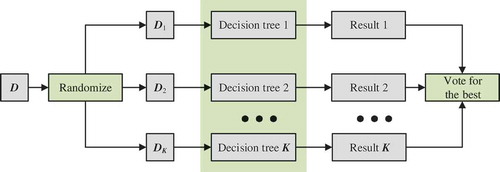
Random Forest is an ensemble learning method composed of K decision trees$\left\{h(X,L_k),k=1,2,\cdots ,K\right\}$, and $\left\{L_k,k=1,2,\cdots ,K\right\}$ is a random vector that is independent and identically distributed, which is used to control the growth of each tree. The algorithm first uses bootstrap sampling to extract k samples from a training set, then establishes a decision tree for each sample, respectively, and finally obtains the sequence$\left\{h_1(X,L_1),h_2(X,L_2),\cdots ,h_k(X,L_k)\right\}$. Under the given independent variable, each decision tree acquires a classification result. The final classification result depends on a simple majority vote for the result of each decision tree. The classification decision can be expressed as

(6) $H(x)=\underset{Y}{argmax}{\sum }_{i=1}^{k}I(h_i(x,L_i)=Y)$(6)

where $H(x)$ represents the combined classification model, $h_i$ is a single decision tree classification model, $I(\cdot )$ is an indicator function, and Y represents the output variable.

3.1.4. Multi-layer perception (MLP)

A MLP is a class of feedforward artificial neural network which consists of at least three layers of nodes (an input and an output layer with one or more hidden layers) with unidirectional connections, often trained by a supervised learning technique (Hannan, Arebey, Begum, Mustafa, & Basri, 2013; Longstaff & Cross, 1987). Each node, except for input nodes, is a neuron that uses a nonlinear activation function. MLP can distinguish data that is not linearly separable, whose multiple layers and nonlinear activation differentiate itself from a linear perceptron.

Learning occurs in the perceptron by changing connection weights after each piece of data is processed, based on the amount of error in the output compared to the expected result, which is constantly carried out through backpropagation. Suppose that the error in output node j in the nth data point is $e_j(n)=d_j(n)-y_j(n)$, where d is the desired output and y is produced by the perceptron. The weights are adjusted based on corrections that minimize the error function, given by $\epsilon (n)=\frac{1}{2}{\sum }_j{e_j}^2(n)$. Using gradient descent, the change in each weight is

(7) $\mathrm{\Delta }{w}_{ji}(n)=-\eta \frac{\mathrm{\partial }\epsilon (n)}{\mathrm{\partial }{v}_j(n)}{y}_i(n),-\frac{\mathrm{\partial }\epsilon (n)}{\mathrm{\partial }{v}_j(n)}=e_j(n){\varphi }^{\prime }(v_j(n))$(7)

where y_i is the output of the previous neuron, $\eta$ is the learning rate, and ${\varphi }^{\prime }$ is the derivative of the activation function. Though the change in weights to a hidden node is complicated, the relevant derivative is

(8) $-\frac{\mathrm{\partial }\epsilon (n)}{\mathrm{\partial }{v}_j(n)}={\varphi }^{\prime }(v_j(n)){\sum }_k-\frac{\mathrm{\partial }\epsilon (n)}{\mathrm{\partial }{v}_k(n)}{w}_{kj}(n)$(8)

This relies on the change in weights of the kth nodes, and the algorithm represents a backpropagation of the activation function.

3.2. Cross-validation method

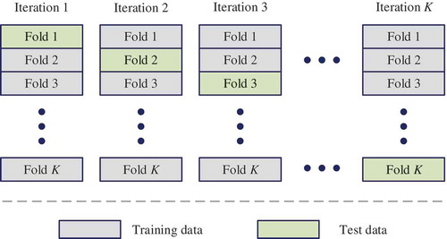
Cross-validation is mainly used in both classification and regression modeling (Arlot & Celisse, 2010; Golub, Heath, & Wahba, 1979). To reduce the bias between the entire dataset and training set (or test set), the K-fold cross-validation method is regarded as the scientific evaluation method for classification modeling. The technique divides the raw dataset into K subsets. One of the subsets is chosen as the test set, and the remaining $K-1$ data subsets are regarded as the training set in each iteration, as shown in Figure 3. Then, the classification accuracy of each classifier is expressed as the average value of the K models obtained from the training number K. Therefore, the K-fold cross-validation method could effectively reduce the randomness of dataset selection and scientifically evaluate the reliability of the classification model.

Figure 3. K-fold cross-validation method.

3.3. Measurement criteria

In order to comprehensively evaluate the classification effect of each classifier, a method combining quantitative and qualitative evaluation is adopted (Pedregosa et al., 2011; Townsend, 1971). On the one hand, the classification accuracy, containing the single and overall classification accuracy, can describe classification results in the form of score. On the other hand, the confusion matrix, as a visual tool, can intuitively exhibit the classification precision (Abdel-Zaher & Eldeib, 2016; Patil & Sherekar, 2013). Both constitute a scientific and rounded evaluation system.

4. Data modeling experiment

4.1. Data collection and filtering

In total, 25,959 basalt samples, containing 2580 MORB, 18363 OIB and 5016 IAB, are collected in this study. There are 12 basic elements for each sample, which are K₂O, CaO, SiO₂, MgO, NiO, Na₂O, FeO^T, TiO₂, Al₂O₃, MnO, Cr₂O₃ and P₂O₅. In these samples, MORB is mainly distributed in the Atlantic and Pacific mid-ocean ridges, OIB is mostly distributed in the Atlantic and Pacific regions, and IAB is principally distributed in the west and east coast of the Pacific rim. Rigorous data filtering is necessary since the basalt samples are from various batches and are acquired by different researchers using diverse instruments. These samples that can be removed are: (1) samples that contain very few basic elements, (2) samples that basic elements have outliers, and (3) samples that affect the balance of the sample size of MORB, OIB and IAB and have more missing values (Wang et al., 2017). Here, 12 basic elements do not need to be filtered in order to study the relationship between geochemical characteristics and tectonic settings. Only 1582 basalt samples containing olivine, the Fo value of which ranges from 36 to 88, remain after data filtering, containing 539 MORB, 463 OIB and 580 IAB, as seen in Table 1. For the convenience of statistics, all of the missing values that remain in the existing samples are replaced with NA in study.

Table 1. Data description of 1582 basalt samples used in this study.

	MORB			OIB			IAB
Elements	Minimum	Maximum	Mean	Minimum	Maximum	Mean	Minimum	Maximum	Mean
K2O	0.01	0.05	0.02	0.00	0.38	0.03	0.00	0.09	0.01
CaO	0.10	0.54	0.31	0.02	0.58	0.31	0.01	0.66	0.21
SiO2	29.93	41.85	40.12	34.71	42.43	39.71	27.32	42.93	39.01
MgO	36.43	51.30	46.64	23.64	51.71	45.47	25.24	52.66	42.65
NiO	0.01	0.44	0.20	0.01	0.43	0.22	0.00	0.55	0.16
Na2O	0.01	0.10	0.02	0.00	0.53	0.14	0.00	0.21	0.02
FeO^T	7.72	23.90	12.59	7.58	42.33	14.28	7.11	37.35	17.18
TiO2	0.01	0.11	0.03	0.00	0.19	0.03	0.00	0.21	0.03
Al2O3	0.01	0.55	0.06	0.00	0.95	0.09	0.00	0.94	0.06
MnO	0.01	0.53	0.20	0.03	0.73	0.21	0.08	0.76	0.27
Cr2O3	0.01	0.21	0.06	0.00	0.23	0.05	0.00	0.29	0.04
P2O5	0.01	0.14	0.07	0.01	0.10	0.03	0.00	0.12	0.02

4.2. Experimental results

Totally, 80% of the existing basalt samples, containing 424 MORB, 374 OIB and 468 IAB, are regarded as the training set and the rest (115 MORB, 89 OIB and 112 IAB) as the test set. The output variables are MORB, OIB and IAB, with the input of 12 basic elements. The critical parameters of each classification model are determined by grid search method. Geochemical discrimination results of tectonic settings of olivine in basalt using LRC, Naïve Bayes, Random Forest and MLP are shown in Table 2 and Figure 4.

Table 2. Discrimination results of tectonic settings of olivine based on four data mining algorithms.

		LRC		Naïve Bayes		Random Forest		MLP
Classes	Test set	Number	Accuracy (%)	Number	Accuracy (%)	Number	Accuracy (%)	Number	Accuracy (%)
MORB	115	86	74.78	102	88.70	99	86.09	102	88.70
OIB	89	49	55.06	36	40.45	60	67.42	72	80.90
IAB	112	96	85.71	89	79.46	104	92.86	104	92.86
Overall	316	231	73.10	227	71.84	263	83.23	278	87.98

* Highlighted in bold denotes the best performance measure of the classifier for each tectonic setting.

Figure 4. Confusion matrixes of geochemical discrimination results of tectonic settings of olivine based on four data mining algorithms: (a) LRC, (b) Naïve Bayes, (c) Random Forest and (d) MLP.

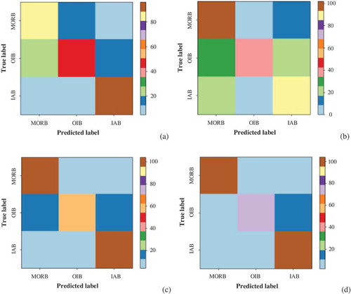
It can be found that the classification accuracy of MORB, OIB and IAB based on MLP is 88.70%, 80.90% and 92.86%, respectively, and the overall classification accuracy is 87.98%. Compared with the other three classifiers, MLP has the best classification effect. The second is Random Forest that has the same IAB classification accuracy as MLP, while the MORB and OIB classification accuracy are lower. The classification performance of LRC and Naïve Bayes is roughly similar. On the whole, though, LRC is better and simpler. However, the results of the constrained experiment have some limitations and the more advanced is necessary.

5. In-depth comparative analysis

5.1. Impact of data preprocessing

5.1.1. Preprocessing techniques

In the whole knowledge discovery process, data preprocessing plays a crucial role before data mining itself. One of the first steps concerns the normalization of the data. This step is very important when dealing with parameters of different units and scales. For example, some data mining techniques use the Euclidean distance. Therefore, all parameters should have the same scale for a fair comparison between them. The min-max normalization and zero-mean standardization are usually well known for rescaling data.

Min-max normalization (Jain & Bhandare, 2011) rescales the values into a range of [0,1]. This might be useful to some extent where all parameters need to have the same positive scale. One possible formula is given below

(9) $X_{normalization}=\frac{X-X_{min}}{X_{max}-X_{min}}$(9)

where X represents each sample data, X_max is the maximum value of sample data, and X_min is the minimum value of sample data.

Zero-mean standardization (Bo, Wang, & Jiao, 2006) transforms data to have zero mean and unit variance. In most cases, standardization is recommended, for example using the equation below

(10) $X_{standardization}=\frac{X-\mu }{\sigma }$(10)

where X represents each sample data, $\mu$ is the mean of sample data, and $\sigma$ is the standard deviation of sample data.

Missing value handling (Frane, 1976) is another important step in data preprocessing. Missing data can distort the classification results and affect the classifier performance. The direct deletion of data containing missing values can result in data waste, thus affecting the generalization ability of the classifier. The imputation method (Donders, van der Heijden, Stijnen, & Moons, 2006) based on statistics replaces the missing value with a certain value, such as mean and mode, so that the data are relatively complete. Since the missing value in the data used is numeric, the missing attribute value can be replaced with the mean of all other values in this attribute.

However, all of these techniques mentioned above have their drawbacks (García, Ramírez-Gallego, Luengo, Benítez, & Herrera, 2016). If you have outliers in your dataset, normalizing your data will certainly scale the normal data to a very small interval. And generally, most of datasets have outliers. When using standardization, your new data are not bounded (unlike normalization). The mean imputation method is easy to implement and does not affect the mean of sample data, but it could reduce the variance of the data, which is not what we want. Therefore, it is necessary to do some research about the impacts of three data preprocessing methods on the classification performance of different classifiers.

5.1.2. Comparison and analysis

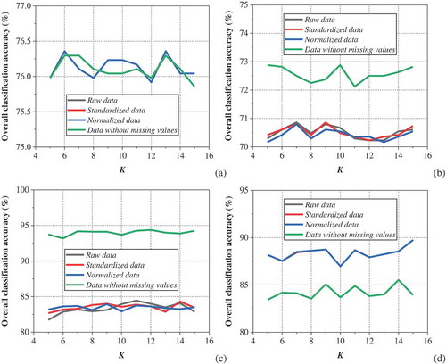
The standardization, normalization and mean imputation methods are applied to the raw geochemical data, respectively, to obtain the standardized, normalized and sound data (equivalent to no missing values). When four classifiers are adopted to discriminate tectonic settings of geochemical data from different preprocessing techniques, the corresponding classification accuracy can be obtained by changing the fold K of the cross-validation method. The classification accuracy can reflect the impacts of different data preprocessing techniques on the classification performance of classifiers. The high precision indicates that the integrated performance of the preprocessing method and the data mining algorithm is better, otherwise the matching effect of the two is not good. In addition, the changes of the overall classification accuracy corresponding to different folds K can show the robustness of the data mining algorithm.

Figure 5 shows the impacts of different preprocessing techniques on the discrimination results of tectonic settings of olivine based on four data mining algorithms, where raw data are considered for a comprehensive comparison. The experimental results are not completely consistent with that in Section 4.2. Different data preprocessing methods have little influence on the classification effect of LRC in Figure 5(a). Figure 5(b) indicates that the mean imputation method raises the classification performance of Naïve Bayes to some extent, while the other two preprocessing methods do not work. It can also be found in Figure 5(c) that the mean imputation method greatly improves the classification accuracy of Random Forest, and the increase is much larger than that of Naïve Bayes, approximately 10%. The standardization and normalization methods are equally ineffective. As shown in Figure 5(d), the mean imputation technique unexpectedly reduces the classification accuracy of MLP, while other techniques remain unchanged. Therefore, the classification accuracy of the combination model of the mean imputation technique and the Random Forest algorithm is the highest, which is about 6% higher than that of the single MLP. Moreover, the maximum difference in classification accuracy of each data mining algorithm is very small within the range of 5 to 15 folds. It turns out that the four classification models are all robust.

Figure 5. Impacts of different data preprocessing techniques on the discrimination results of tectonic settings of olivine based on four data mining algorithms: (a) LRC, (b) Naïve Bayes, (c) Random Forest, and (d) MLP.

5.2. Feature importance measurement

5.2.1. Principle description

There are 12 basic elements as classification features in the geochemical data of olivine. It is a crucial issue that how to select features that have the most influence on the tectonic setting discrimination results, thus reducing features in modeling. There are many ways to do this, and Random Forest is one of them. The idea is to use the Gini index to measure the contribution of each feature to each tree in a random forest, and then take the mean to obtain the importance score of each feature (Granitto, Furlanello, Biasioli, & Gasperi, 2006; Menze et al., 2009).

Suppose that there are c features $X_1,X_2,\cdots ,X_c$ in total, and the Gini index (GI) score for feature X_j is $FI{M_j}^{(Gini)}$, that is the abbreviation for feature importance measures. The formula of Gini index is $G{I}_m=1-{\sum }_{k=1}^{\left|K\right|}{p}_{mk}^2$, where K denotes the number of categories, and p_mk represents the proportion of category k in node m. The importance of feature X_j in node m, that is, the change of Gini index before and after node m branching is $FI{M_{jm}}^{(Gini)}=G{I}_m-G{I}_l-G{I}_r$, where GI_l and GI_r represent the Gini index of two new nodes after branching, respectively. The nodes that feature X_j appears in decision tree i are in set M, then the importance of X_j in the ith tree is $FI{M_{ij}}^{(Gini)}={\sum }_{m\in M}FI{M_{jm}}^{(Gini)}$. There are n trees in a random forest, so the importance of X_j is $FI{M_j}^{(Gini)}={\sum }_{i=1}^{n}FI{M_{ij}}^{(Gini)}$. All of the importance scores obtained are finally normalized, i.e. $FI{M_j}^{(Gini)}=\frac{FI{M}_j}{{\sum }_{i=1}^{c}FI{M}_i}$.

5.2.2. Results and discussion

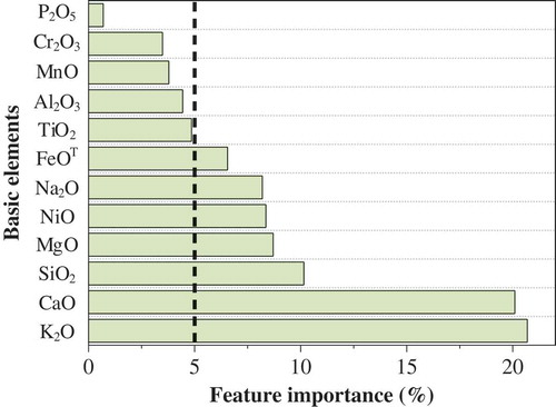
According to the method described in Section 5.2.1, the importance score of each basic element of the olivine in basalt samples is summarized, as shown in Figure 6. As you can see in the figure, the sum of the feature importance ($>5\mathrm{\%}$) of the seven basic elements, including K₂O, CaO, SiO₂, MgO, NiO, Na₂O and FeO^T, has exceeded 0.80. This indicates that these seven basic elements play a role of over 80% in the process of tectonic setting discrimination, which should be given more attention in the following studies. However, there are doubts about the order of the feature importance of 12 basic elements. On the one hand, Section 5.1 has proven that the mean imputation method does affect the performance of a classifier. Figure 5 illustrates this intuitively. On the other hand, Table 1 and Figure 6 show that the number of missing values for an element might influence its importance score. For example, P₂O₅ is the least important element, with a miss rate of up to 93%. Although Na₂O is the sixth important element now, it may be more important as the number of missing values decreases. The only exception is that though there are many missing values for K₂O, it is still the most important. In view of these points, relatively large amounts of complete data need to be collected to achieve more reliable evaluation results of the feature importance. Therefore, the order of the feature importance of basic elements shown in Figure 6 is only for the geochemical data used in this study.

Figure 6. Feature importance evaluation results of 12 basic elements using Random Forest.

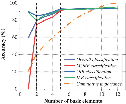
In order to quantitatively measure the contribution of each basic element to the model classification performance, all of the elements are sorted by feature importance from large to small, and the simulation experiment is carried out by adding them one by one. There are 12 experimental conditions in all, as illustrated in Table 3. The sum of the feature importance of corresponding basic elements under each condition is listed in the table, for the convenience of studying the relationship between the cumulative feature importance and the single and overall classification accuracy. And also, the 10-fold cross-validation method and the combination model of the mean imputation technique and the Random Forest algorithm are adopted in this experiment.

Table 3. Combination results of basic elements on the basis of feature importance measurement.

Number	Combination of basic elements (note that feature importance goes from large to small)	Sum of feature importance (%)
1	K2O	20.69
2	K2O, CaO	40.78
3	K2O, CaO, SiO2	50.93
4	K2O, CaO, SiO2, MgO	59.64
5	K2O, CaO, SiO2, MgO, NiO	68.00
6	K2O, CaO, SiO2, MgO, NiO, Na2O	76.19
7	K2O, CaO, SiO2, MgO, NiO, Na2O, FeO^T	82.74
8	K2O, CaO, SiO2, MgO, NiO, Na2O, FeO^T, TiO2	87.60
9	K2O, CaO, SiO2, MgO, NiO, Na2O, FeO^T, TiO2, Al2O3	92.04
10	K2O, CaO, SiO2, MgO, NiO, Na2O, FeO^T, TiO2, Al2O3, MnO	95.82
11	K2O, CaO, SiO2, MgO, NiO, Na2O, FeO^T, TiO2, Al2O3, MnO, Cr2O3	99.31
12	K2O, CaO, SiO2, MgO, NiO, Na2O, FeO^T, TiO2, Al2O3, MnO, Cr2O3, P2O5	100.00

The experimental results are summarized in Figure 7. When the input variable is only K₂O, the classification accuracy of MORB is 0, while the classification accuracy of OIB and IAB are both as high as 90%. The overall classification accuracy is just 60% due to the poor classification effect of MORB. The number of missing values for 12 basic elements in different tectonic settings is listed in Table 4. Both MORB and IAB have higher miss rate, and it is obvious that the missing value has greater effects on MORB. On the other hand, when the number of elements is between two and five, the single and overall classification accuracy increase with the rise of the number of elements. The classification effect remains stable when the number of elements is greater than five. The number of missing values has little effect on the classification accuracy in these two cases because there exists no mutation. As a whole, the change trends of both the cumulative feature importance and the classification accuracy are not entirely consistent. The accumulative feature importance is increasing all the time, while the classification accuracy improves at the beginning and then keeps steady.

Table 4. Number of missing values for 12 basic elements in different tectonic settings.

	Number of missing values
Basic elements	MORB (539)	OIB (463)	IAB (580)	Total (1582)
K2O	441	0	480	921
CaO	0	1	0	1
SiO2	0	0	0	0
MgO	0	0	0	0
NiO	266	88	0	354
Na2O	380	182	423	985
FeO^T	0	0	0	0
TiO2	362	144	2	508
Al2O3	0	88	0	88
MnO	0	5	0	5
Cr2O3	0	0	0	0
P2O5	503	433	535	1471

*(·) denotes the total number of basalt samples for each tectonic setting.

Figure 7. Impacts of different combinations of basic elements (note that feature importance goes from large to small) on the discrimination results of tectonic settings of olivine based on Random Forest.

5.3. Differences in sample data

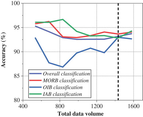
Sample data volume is not only related to the accuracy of tectonic setting discrimination but also connected with the deployment of computing resource. It is imperative to research on the effects of sample data volumes on the classification accuracy. To this end, the following simulation experiment is conducted. The sample data volume of MORB, OIB and IAB is reduced by 50 at a time, respectively, that is, the total number is reduced by 150 every time. A total of eight experimental conditions are formed. The 5-fold cross-validation method and the combination model of the mean imputation technique and the Random Forest algorithm are adopted in each case. All the experimental conditions and results are shown in Table 5. Furthermore, Figure 8 depicts the relationship between the total data volume and the single and overall classification accuracy. As can be clearly seen from the picture, the single and overall classification accuracy roughly decrease first and then improve with the increase of the total data volume. The classification accuracy of OIB is more influenced by data volume than that of others. It is also found that each classification accuracy tends to be stable when the data volume is over 1400. In summary, the appropriate data volume is selected for tectonic setting discrimination, which can reduce the computing power and time consumption without affecting the discrimination accuracy.

Table 5. Single and overall classification accuracy for different sample data volumes.

Sample data volume				Classification accuracy (%)
Total	MORB	OIB	IAB	Overall	MORB	OIB	IAB
532	189	113	230	95.30	95.77	92.92	96.09
682	239	163	280	94.13	96.23	87.73	96.07
832	289	213	330	92.91	93.08	86.85	96.67
982	339	263	380	92.57	92.92	89.73	94.21
1132	389	313	430	92.58	93.32	90.73	93.26
1282	439	363	480	92.59	94.08	89.81	93.33
1432	489	413	530	93.16	93.66	92.98	92.83
1582	539	463	580	93.74	94.06	92.66	94.31

Figure 8. Impacts of different sample data volumes on the discrimination results of tectonic settings of olivine based on Random Forest.

6. Conclusions and future works

The data mining technique is introduced to discriminate tectonic settings of the olivine in basalt in this paper. From this case, the effects of different data preprocessing methods, combinations of geochemical characteristics and sample data volumes on the model classification performance are also studied. The results show that the data mining algorithm has comparable advantages in tectonic setting discrimination, mainly including the following:

1. It has been preliminarily proved that the composition of olivine in basalt has the function of discriminating tectonic settings. However, the initial finding obtained by the data-driven method needs further examination, because some scholars still do not believe that olivine is closely related to the tectonic setting where it formed.

2. The combination model of the mean imputation technique and the Random Forest algorithm is recommended for discriminating tectonic settings of olivine in basalt. Nevertheless, a single MLP is worth considering if the number of missing values is small.

3. The seven basic elements, including K₂O, CaO, SiO₂, MgO, NiO, Na₂O and FeO^T, play a role of over 80% in the course of tectonic setting discrimination of olivine in basalt. It is worth mentioning that the first five basic elements are enough to achieve good classification effects.

4. The classification accuracy of OIB is more influenced by the data volume. The single and overall classification accuracy can reach the large and stable value when the data volume is over 1400. The more appropriate data volume calls for more research.

It is convenient and accurate to discriminate tectonic settings by data mining algorithms, which is worth spreading in geochemistry. However, it remains to be studied that how to explain potential patterns obtained from data mining scientifically and reasonably.

Data availability statement

The data referred to in this paper is not publicly available at the current time.

Disclosure statement

No potential conflict of interest was reported by the authors.

Additional information

Funding

This research was supported by the Tianjin Science Foundation for Distinguished Young Scientists of China [Grant No. 17JCJQJC44000] and the National Natural Science Foundation for Excellent Young Scientists of China [Grant No. 51622904].

References

- Abdel-Zaher, A. M., & Eldeib, A. M. (2016). Breast cancer classification using deep belief networks. Expert Systems with Applications, 46, 139–144.
- Arevalo, R., McDonough, W. F., & Luong, M. (2009). The K/U ratio of the silicate Earth: Insights into mantle composition, structure and thermal evolution. Earth and Planetary Science Letters, 278(3), 361–369.
- Arlot, S., & Celisse, A. (2010). A survey of cross-validation procedures for model selection. Statistics Surveys, 4, 40–79.
- Bhatia, M. R., & Crook, K. A. (1986). Trace element characteristics of graywackes and tectonic setting discrimination of sedimentary basins. Contributions to Mineralogy and Petrology, 92(2), 181–193.
- Bo, L., Wang, L., & Jiao, L. (2006). Feature scaling for kernel fisher discriminant analysis using leave-one-out cross validation. Neural Computation, 18(4), 961–978.
- Breiman, L. (2001). Random forests. Machine Learning, 45(1), 5–32.
- Di, P., Wang, J., Zhang, Q., Yang, J., Chen, W., Pan, Z., … Jiao, S. (2017). The evaluation of basalt tectonic discrimination diagrams: Constraints on the research of global basalt data. Bulletin of Mineralogy, Petrology and Geochemistry, 36(6), 891–896.
- Donders, A. R. T., Van Der Heijden, G. J., Stijnen, T., & Moons, K. G. (2006). A gentle introduction to imputation of missing values. Journal of Clinical Epidemiology, 59(10), 1087–1091.
- Enciso-Maldonado, L., Dyer, M. S., Jones, M. D., Li, M., Payne, J. L., Pitcher, M. J., … Rosseinsky, M. J. (2015). Computational identification and experimental realization of lithium vacancy introduction into the olivine LiMgPO4. Chemistry of Materials, 27(6), 2074–2091.
- Frane, J. W. (1976). Some simple procedures for handling missing data in multivariate analysis. Psychometrika, 41(3), 409–415.
- García, S., Ramírez-Gallego, S., Luengo, J., Benítez, J. M., & Herrera, F. (2016). Big data preprocessing: Methods and prospects. Big Data Analytics, 1(1), 9.
- Golub, G. H., Heath, M., & Wahba, G. (1979). Generalized cross-validation as a method for choosing a good ridge parameter. Technometrics, 21(2), 215–223.
- Granitto, P. M., Furlanello, C., Biasioli, F., & Gasperi, F. (2006). Recursive feature elimination with random forest for PTR-MS analysis of agroindustrial products. Chemometrics and Intelligent Laboratory Systems, 83(2), 83–90.
- Han, S., Li, M., Ren, Q., & Liu, C. (2018). Intelligent determination and data mining for tectonic settings of basalts based on big data methods. Acta Petrologica Sinica, 34(11), 3207–3216.
- Hannan, M. A., Arebey, M., Begum, R. A., Mustafa, A., & Basri, H. (2013). An automated solid waste bin level detection system using Gabor wavelet filters and multi-layer perception. Resources, Conservation and Recycling, 72, 33–42.
- Howarth, G. H., & Harris, C. (2017). Discriminating between pyroxenite and peridotite sources for continental flood basalts (CFB) in southern Africa using olivine chemistry. Earth and Planetary Science Letters, 475, 143–151.
- Jain, Y. K., & Bhandare, S. K. (2011). Min max normalization based data perturbation method for privacy protection. International Journal of Computer and Communication Technology, 2(8), 45–50.
- Li, C., Arndt, N. T., Tang, Q., & Ripley, E. M. (2015). Trace element indiscrimination diagrams. Lithos, 232, 76–83.
- Li, M., Miao, L., & Shi, J. (2014). Analyzing heating equipment’s operations based on measured data. Energy and Buildings, 82, 47–56.
- Longstaff, I. D., & Cross, J. F. (1987). A pattern recognition approach to understanding the multi-layer perception. Pattern Recognition Letters, 5(5), 315–319.
- Luo, J., Wang, X., Song, B., Yang, Z., Zhang, Q., Zhao, Y., & Liu, S. (2018). Discussion on the method for quantitative classification of magmatic rocks: Taking it’s application in West Qinling of Gansu Province for example. Acta Petrologica Sinica, 34(2), 326–332.
- Menze, B. H., Kelm, B. M., Masuch, R., Himmelreich, U., Bachert, P., Petrich, W., & Hamprecht, F. A. (2009). A comparison of random forest and its Gini importance with standard chemometric methods for the feature selection and classification of spectral data. BMC Bioinformatics, 10(1), 213.
- Mitchell, T. M. (2005). Generative and discriminative classifiers: Naive Bayes and logistic regression. Machine Learning. New York: McGraw Hill.
- Patil, T. R., & Sherekar, S. S. (2013). Performance analysis of Naive Bayes and J48 classification algorithm for data classification. International Journal of Computer Science and Applications, 6(2), 256–261.
- Pearce, J. A. (1996). A user’s guide to basalt discrimination diagrams. Trace element geochemistry of volcanic rocks: Applications for massive sulphide exploration. Geological Association of Canada, Short Course Notes, 12, 79–113.
- Pearce, J. A., & Cann, J. R. (1973). Tectonic setting of basic volcanic rocks determined using trace element analyses. Earth and Planetary Science Letters, 19(2), 290–300.
- Pedregosa, F., Varoquaux, G., Gramfort, A., Michel, V., Thirion, B., Grisel, O., … Duchesnay, É. (2011). Scikit-learn: Machine learning in Python. Journal of Machine Learning Research, 12(10), 2825–2830.
- Petrelli, M., & Perugini, D. (2016). Solving petrological problems through machine learning: The study case of tectonic discrimination using geochemical and isotopic data. Contributions to Mineralogy and Petrology, 171(10), 81.
- Ren, Q., Wang, G., Li, M., & Han, S. (2019). Prediction of rock compressive strength using machine learning algorithms based on spectrum analysis of geological hammer. Geotechnical and Geological Engineering, 37(1), 475–489.
- Sánchez-Muñoz, L., Müller, A., Andrés, S. L., Martin, R. F., Modreski, P. J., & de Moura, O. J. (2017). The P-Fe diagram for K-feldspars: A preliminary approach in the discrimination of pegmatites. Lithos, 272, 116–127.
- Subasi, A., & Ercelebi, E. (2005). Classification of EEG signals using neural network and logistic regression. Computer Methods and Programs in Biomedicine, 78(2), 87–99.
- Taalab, K., Cheng, T., & Zhang, Y. (2018). Mapping landslide susceptibility and types using Random Forest. Big Earth Data, 2(2), 159–178.
- Townsend, J. T. (1971). Theoretical analysis of an alphabetic confusion matrix. Perception & Psychophysics, 9(1), 40–50.
- Ueki, K., Hino, H., & Kuwatani, T. (2018). Geochemical discrimination and characteristics of magmatic tectonic settings: A machine-learning-based approach. Geochemistry, Geophysics, Geosystems, 19(4), 1327–1347.
- Vermeesch, P. (2006). Tectonic discrimination of basalts with classification trees. Geochimica et Cosmochimica Acta, 70(7), 1839–1848.
- Wang, J., Chen, W., Zhang, Q., Jiao, S., Yang, J., Pan, Z., & Wang, S. (2017). Preliminary research on data mining of N-MORB and E-MORB: Discussion on method of the basalt discrimination diagrams and the character of MORB’s mantle source. Acta Petrologica Sinica, 33(3), 993–1005.
- Zhang, Q. (1990). The correct use of the basalt discrimination diagram. Acta Petrologica Sinica, 2, 87–94.
- Zhou, X., Chen, Z., & Chen, T. (1980). Composition and evolution of olivine and pyroxene in alkali basaltic rocks from Jiangsu Province. Geochimica, 33(3), 253–262.
- Zhou, Y., Chen, S., Zhang, Q., Xiao, F., Wang, S., Liu, Y., & Jiao, S. (2018). Advances and prospects of big data and mathematical geoscience. Acta Petrologica Sinica, 34(2), 255–263.