A generalized supervised classification scheme to produce provincial wetland inventory maps: an application of Google Earth Engine for big geo data processing

ABSTRACT

Wetlands are important natural resources due to their numerous ecological services. Consequently, identifying their locations and extents is imperative. The stability, repeatability, cost-effectiveness, multi-scale coverage, and proper spatial resolution imagery of satellites provide a valuable opportunity for their use in various large-scale applications, such as provincial wetland mapping. To do so, it is required to (1) process and classify big geo data (i.e. a large amount of satellite datasets) in a time- and computationally-efficient approach and (2) collect a large amount of field samples. In this study, Google Earth Engine (GEE) and machine learning algorithms were utilized to process thousands of remote sensing images and produce provincial wetland inventory maps of the three Canadian provinces of Manitoba, Quebec, and Newfoundland and Labrador (NL). Additionally, using GEE, a generalized supervised classification method is proposed to produce a regional wetland map from a large area (e.g., a province) when lacking field samples. In fact, using the field data from only Manitoba and assuming that all wetlands in Canada have similar characteristics, the wetland maps were generated for the other two provinces. The overall classification accuracies for Manitoba, Quebec, and NL were 84%, 78%, and 82%, respectively, indicating the high potential of the proposed method for aiding provincial wetland inventory systems.

KEYWORDS:

• Wetlands
• remote sensing
• Google Earth Engine
• big geo data
• image classification

1. Introduction

As the kidneys of environment, wetlands are among the most productive landscapes on Earth. These valuable ecosystems provide numerous services to environment and humans. They are also the natural habitat of numerous types of flora and fauna, which include one third of at-risk species (Mahdavi et al., 2018). Additionally, they purify water and remove pollutants, protect shorelines, store atmospheric carbon, and enhance biodiversity (Mitsch & Gosselink, 2000; Ozesmi & Bauer, 2002). However, despite their importance, wetlands are being degraded and lost due to human activities and climate change. As early as the 1700’s, for example, the Mi’gmaq living near the Bay of Fundy, New Brunswick, Canada noted and complained about the reduced amounts of duck and geese available for hunting after extensive destruction of salt marshes in the area (McAlpine & Smith, 2010). Consequently, it is pivotal to monitor and protect wetlands using regularly updated, high resolution, and large-scale wetland maps. In this regard, remote sensing provides an excellent opportunity to identify the locations and extent of wetlands. Free time series optical and Synthetic Aperture RADAR (SAR) datasets, including those acquired by Landsat-8, Sentinel-1, and Sentinel-2 are the most promising resources for classifying wetlands over large areas and monitoring their changes over time (Shelestov, Lavreniuk, Kussul, Novikov, & Skakun, 2017).

The necessity of wetland conservation is reflected in several international and global efforts. For instance, serious endeavors to prevent or ameliorate wetland loss in North America began in the 1970s (Mahdavi et al., 2019; Mitsch & Gosselink, 2000). Since then, numerous studies have demonstrated that remote sensing is the only practical option for producing frequent wetland maps over large areas and various inventory systems (Mitsch & Gosselink, 2000; Ozesmi & Bauer, 2002). In country- or province-wide wetland mapping using satellite images, it is important to consider processing big geo data in the classification procedure (e.g. thousands of satellite images) over a large area. This is not possible using conventional software packages and programming languages. Several platforms, such as Google Earth Engine (GEE), NASA Earth Exchange, Amazon’s Web Services, and Microsoft’s Azure have been created to tackle this issue and facilitate manipulation and analysis of big geo data (Amani et al., 2019; Hird, DeLancey, McDermid, & Kariyeva, 2017; Xiong et al., 2017). Particularly, Google has launched GEE, one of the applications of which is processing big geospatial data and classifying land cover over broad regions (Gorelick et al., 2017). In this platform, the open source images acquired by several satellites, including Sentinel-1, −2, Landsat-8, and MODIS are accessible and can be efficiently imported and processed in the cloud without the necessity of downloading the data to local computers. Moreover, several image-driven products and many remote sensing algorithms, including classification algorithms and cloud masking methods, are available in this platform and are readily included and editable in user-defined algorithms (Gorelick et al., 2017; Kumar & Mutanga, 2018). To date, several studies have been conducted around the world for large-scale classifications using GEE. For instance, Lobell, Thau, Seifert, Engle, and Little (2015) proposed a satellite-based Scalable Crop Yield Mapper (SCYM) to combine weather data and Landsat images within GEE to estimate crop yields. Additionally, Zhang, Li, Thau, and Moore (2015) applied daytime Landsat Normalized Difference Vegetation Index (NDVI) and nighttime Defense Meteorological Satellite Program/Operational Linescan System (DMSP/OLS) light imagery to identify global urban areas at 30 m spatial resolution using GEE. Finally, Pekel, Cottam, Gorelick, and Belward (2016) applied three million Landsat images within GEE to monitor the changes in global surface water over 32 years. Specifically, they identified the times that water was present globally, where the changes occurred, and what forms of changes in terms of seasonality and persistence occurred.

A large portion of Canada is covered by wetlands and, thus, numerous studies have classified and assessed them using remotely sensed data in different provinces (e.g. Amani et al., 2018a; Brisco et al., 2013; Dabboor, White, Brisco, & Charbonneau, 2015; White, Brisco, Dabboor, Schmitt, & Pratt, 2015). Most of these studies focused on relatively small areas and were developed for different purposes. To date, several studies have classified wetlands in Canada at large scales (e.g. https://maps.alberta.ca/genesis/rest/services/Alberta_Merged_Wetland_Inventory/Latest/MapServer/; https://www.ducks.ca/resources/industry/enhanced-wetland-classification-inferred-products-user-guide/; Wulder et al., 2018), only a few of which have investigated GEE for this purpose (e.g. https://www.mae.gov.nl.ca/waterres/rti/rtwq/workshops.html#2018; Amani et al., 2019; Hird et al., 2017). For example, Hird et al. (2017) were the first that applied GEE to estimate the probability of wetland occurrence in a 13,700 km² region in Alberta. Later, Amani (2018) presented the first Canadian provincial wetland inventory map over the province of Newfoundland and Labrador (NL) with an area of 405,212 km². The author used Landsat-8 imagery available in GEE along with several field samples to identify the locations of the five main wetland classes specified by the Canadian Wetland Classification System (CWCS): Bog, Fen, Marsh, Swamp, Shallow Water. Finally, Amani et al. (2019) applied 30,000 Landsat-8 imagery collected from 2016 to 2018 along with large amount of field samples to produce the first Canadian Wetland Inventory (CWI) map based on the CWCS specifications. This study was the first to produce a Canada-wide wetland map (~10 million km²) including updated and comprehensive information about the location and extent of wetlands across the entire country. Using the Random Forest (RF) algorithm, the overall classification accuracy was 71% and the average producer and user accuracies for only wetland classes were 66% and 63%, respectively.

As discussed above, GEE offers a novel opportunity for large-scale wetland mapping and its application for classifying Canadian wetlands is growing. One of the issues with wetland mapping in some parts of the Canada is the lack of proper field samples with which to validate remote sensing and supervised image classification algorithms. Additionally, the accuracy of the available large-scale maps of Canadian wetlands are relatively low. Therefore, a generalized supervised classification scheme was proposed in this study to produce province-wide wetland inventory maps of provinces that lack field samples. To this end, the field data collected from Manitoba were used to create Manitoba-, Quebec-, and NL-wide wetland maps. Moreover, a combination of optical, SAR, and Canadian Digital Elevation Model (CDEM) data, which is considered the best combination for wetland mapping, was used to produce improved wetland maps of these three Canadian provinces. The produced maps were the improved Manitoba-, Quebec-, NL-wide wetland maps. Finally, it should be noted that the proposed generalized method is helpful for creating wetland inventory maps of any Canadian province without field samples given the land cover and specifically wetland classes are similar.

2. Study areas and datasets

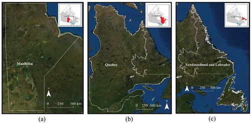
The study areas included the three Canadian provinces of Manitoba, Quebec, and NL, which are illustrated in Figure 1 and explained in subsection 2.1. Furthermore, the three remote sensing datasets, including Landsat-8, Sentinel-1, and CDEM, used in this study to classify wetlands, are discussed in subsection 2.2.

Figure 1. Study areas: (a) Manitoba, (b) Quebec, (c) Newfoundland and Labrador. The maps were adopted from https://www.nrcan.gc.ca/earth-sciences/geography/atlas-canada/explore-our-maps/reference-maps/16846.

2.1. Study areas

Manitoba is a province in Canada with a central latitude and longitude of 53.76° N and 98.81° W, respectively, and a total area of approximately 649,950 km². This province has a continental climate, flat geography, and generally possesses the five ecozones of boreal plains, prairie, taiga shield, boreal shield, and Hudson. Manitoba is a province rich in wetlands, including bogs and fens, wetlands in the margins of rivers and lakes, and coastal areas (Amani et al., 2019).

Québec is the second largest province in Canada with a central latitude of 52.94° N and 73.55° W, respectively. Due to Québec’s large area (approximately 1,542,056 km²), its geography varies by region. Québec has three main climates, including humid continental, subarctic, and arctic. The most common land cover types in this province are tundra, taiga, various types of forests, and wetlands (Amani et al., 2019).

NL is another province within Canada, the center of which has the coordinates of 53.14° N and 57.66° W with a total area of 405,720 km². NL has different climates, including oceanic, continental, and humid-continental due to its geography. Various land covers, including peatlands, permafrost, heathland barrens, balsam fir, black spruce, and white birch forests are found in NL (Mahdavi et al., 2017). It is estimated that a large portion of this province is covered by various types of wetlands, especially bogs and fens (Amani et al., 2019).

2.2. Field data

The CWCS divides Canadian wetlands into the five classes of Bog, Fen, Marsh, Swamp, and Shallow Water (Warner & Rubec, 1997). Thus, in the final wetland inventory maps, there are five main wetland classes along with five non-wetland classes, which are found throughout the study areas. Field samples in this study were provided by different organizations, including Environment and Climate Change Canada (ECCC), Ducks Unlimited Canada (DUC), Northeast Avalon Atlantic Coastal Action Program, and the Memorial University of Newfoundland. The field samples were collected by these organizations between the years of 2000 to 2018. The field samples were visually checked against existing high-resolution imagery to ensure their land use had not changed to urban or agriculture. Then, the polygons for field samples were delineated and created in ArcGIS, the details of which are provided in Table 1. As clear from this table, the field samples collected from Manitoba were divided into two groups of training and test (50/50%), while the field samples from the other two provinces were only used for accuracy assessment of the classified maps from these two provinces.

Table 1. The number and area of field polygons used in this study. Note that the samples from Manitoba were approximately divided into 50/50% (training and test datasets), while the field data from Quebec and Newfoundland and Labrador (NL) were only used for accuracy assessment of their classified maps.

	Manitoba				Quebec		NL
	Training data		Test data		Test data		Test data
Class*	#polygons	Area (km^2)	#polygons	Area (km^2)	#polygons	Area (km^2)	#polygons	Area (km^2)
Bog	6	26.1	6	24.2	12	25.7	45	10.6
Fen	9	38.2	8	39.1	5	7.4	32	4.2
Marsh	4	24.4	4	22.2	7	27.6	70	8.5
Swamp	7	24.1	7	21.3	16	25.6	28	2.0
Shallow Water^a	11	11.0	10	10.3	9	36.0	54	3.1
Deep Water	5	27.6	5	23.9	5	21.2	41	11.4
Forest^b	18	36.9	15	30.0	8	14.9	37	15.1
Grassland^c	8	39.4	7	32.3	12	17.2	45	2.9
Cropland	6	28.4	6	23.6	25	25.4	16	0.8
Baren^d	30	15.7	30	18.3	6	20.5	25	19.6

^aWater bodies with less than 2m depth.

^bThis class includes deciduous, coniferous, and mixedwood forests.

^cThis class includes grassland, pasture, cropland, shrubland, and heathland.

^dThis class includes urban, road, rock, sand, gravel, and other bare land covers.

*See Amani et al. (2018a) for a detailed description of different wetland classes.

2.3. Satellite data

A combination of freely available multi-source and multi-temporal optical (Landsat-8), SAR (Sentinel-1), and elevation (CDEM) imagery were used in the classifications. Six spectral bands of Landsat-8, including visible, Near Infrared (NIR), and Shortwave Infrared (SWIR) channels with 30 m spatial resolution were used. These images were collected between May 1 to November 30 in 2016, 2017, and 2018. It is worth noting that the imagery from three years were used in this study because this was the minimum number of years that a non-cloud mosaic image could be created from the study areas. For instance, if the Landsat-8 imagery from two years are used over the study areas, there will be several cloudy areas in the final classified maps. Furthermore, the Sentinel-1 images, acquired between May 1 to November 30 in 2016, 2017, and 2018, with the Interferometric Wide (IW) swath mode, VV and VH polarizations, and 10 m spatial resolution were employed in this study. The CDEM data were produced by Natural Resources Canada (NRCan) and the elevations were either ground or reflective surface elevations (NRCan, 2016). Although the resolution of CDEM varies based on the altitude, it generally has a spatial resolution of 0.75 arc sec (20 m).

3. Methodology

The proposed methodology included satellite data preprocessing, defining the optimal classification features, classifying the land covers, and assessing the accuracy of the classifications. All the steps of the proposed methodology were implemented in GEE and are discussed in more detail in the following subsections.

3.1. Satellite data preprocessing

The atmospherically corrected Landsat-8 optical imagery available in GEE (Tier 1 products, ee.ImageCollection(“LANDSAT/LC08/C01/T1_SR”)) were employed in this study. These products are atmospherically corrected using the Landsat-8 Surface Reflectance Code (LaSRC) and contain cloud, shadow, water, and snow masks, which are generated using the C Function of Mask (CFMask) algorithm (Foga et al., 2017). The LaSRC algorithm applies a modified version of the 6SV relative transfer code along with an accurate method for aerosol estimation (Vermote, Justice, Claverie, & Franch, 2016). Another important fact which should be considered in Canada is cloud and snow masking when optical imagery is used in the classification. Canadian provinces are prone to frequent cloud coverage and snowfall and, therefore, adopting an efficient method for cloud and snow removal from Landsat-8 images is challenging. Since multi-date images over three years were used in this research, cloud- and snow-contaminated areas were effectively removed from the images. To do so, a JavaScript code in GEE was applied to all Landsat-8 imagery, acquired between May 1 to November 30 in 2016, 2017, and 2018, in which a median ee.Reducer function was used. This was performed to downscale all the collected information into a single image for which the pixel values represented the median of the image pixels containing no or minimum snow/cloud. Additionally, by doing this, pixels that were too dark or too bright were removed.

SAR data, such as those acquired by the Sentinel-1 satellite, have demonstrated high potential for discriminating wetland classes in many studies (e.g. Hird et al., 2017;). Sentinel-1 collects data with different swath widths, spatial resolutions, and polarizations during both ascending and descending orbits. It was necessary to filter these datasets to obtain a homogenous subset in GEE. The primary mode of Sentinel-1 data over land is IW swath mode with VV and VH polarizations (https://sentinel.esa.int/web/sentinel/user-guides/sentinel-1-sar/acquisition-modes). Moreover, the ascending orbit is more suitable for wetland classification compared to the descending mode due to the presence of dew at the time of descending image acquisition which decreases the contrast between wetland and non-wetland species (Grenier et al., 2007). Therefore, the Sentinel-1 images with VV and VH polarizations, IW swath mode, and ascending orbit with a 10 m spatial resolution were employed in this work. Specifically, the C-band Sentinel-1 Ground Resolution Detected (GRD) datasets available within GEE (ee.ImageCollection(“COPERNICUS/S1_GRD”)) were adopted. These products are calibrated and ortho-corrected using Sentinel-1 Toolbox (https://sentinel.esa.int/web/sentinel/toolboxes/sentinel-1). The GRD border noise removal, thermal noise removal, radiometric calibration, and terrain correction were performed on these datasets (see https://developers.google.com/earth-engine/sentinel1 for more details). Therefore, the only necessary preprocessing step applied to these images was speckle reduction. It has been argued in many studies that the refined Lee filter provided high potential for speckle reduction (e.g. Amani, Salehi, Mahdavi, Brisco, & Shehata, 2018b; Lee, Grunes, & De Grandi, 1999) and, therefore, a 7 × 7 refined Lee filter implemented by Guido Lemoine within GEE (https://code.earthengine.google.com/2ef38463ebaf5ae133a478f173fd0ab5) was utilized in this study.

3.2. Features

It is important to include the most optimal features into the classification to obtain a highly accurate wetland map. Based on our previous studies (e.g. Amani et al., 2018a), the optical, SAR, and elevation features listed in Table 2 (13 features in total) have the highest potential to discriminate various wetland species and, thus, were used in this study. For instance, the NIR band is the most useful for identifying vegetation and water, both of which are important characteristics of wetlands and, thus, this an important band for wetland classification (Ozesmi & Bauer, 2002). Moreover, the SWIR band is helpful in detecting moisture contents in vegetation and soil and, therefore, is important for discriminating non-wetlands from wetlands, which are usually wet (Crist & Cicone, 1984). The visible bands, especially the red band, also demonstrated potential for detecting wetland classes. For instance, bog contains sphagnum moss, which has a red/orange appearance and, consequently, this is one of the most accurate bands for detecting this wetland class (Amani et al., 2018a). In terms of SAR features, VV polarization is useful for detecting flooded wetlands and VH polarization is helpful in discriminating between herbaceous and woody wetlands, such as the Marsh and Swamp classes (Henderson & Lewis, 2008). The ratio feature of VV/VH has also proved promising for identifying non-forested wetlands (Bourgeau-Chavez, Riordan, Powell, Miller, & Nowels, 2009). In addition, it has been widely recognized that elevation data is considerably important for identifying wetlands (Chasmer, Hopkinson, Montgomery, & Petrone, 2016; Hird et al., 2017; Huang, Peng, Lang, Yeo, & McCarty, 2014) because wetlands are usually located in flat areas. In this study, the free CDEM data available in GEE was used in this study.

Table 2. The optical, SAR, and elevation features applied to the classifications in this study.

Satellite	Features
Landsat-8	Main channels: Spectral indices:	B2 (blue), B3 (Green), B4 (Red), B5 (NIR), B6 (SWIR-1), B7 (SWIR-2) $NDWI=\frac{Green-NIR}{Green+NIR}$, $NDVI=\frac{NIR-Red}{NIR+Red}$, $NDSI=\frac{SWIR-NIR}{SWIR+NIR}$
Sentinel-1	Main channels:	VV, VH
	Ratio features:	$\frac{VV}{VH}$
	Elevation	Canadian Digital Elevation Model
B: Band SWIR: Shortwave Infrared NDVI: Normalized Difference Vegetation Index VH: Vertical transmit and Horizontal receive polarizations			NIR: Near Infrared NDWI: Normalized Difference Water Index NDSI: Normalized Difference Soil Index VV: Vertical transmit and Vertical receive polarizations

3.3. Classification

The features mentioned in Table 2 were inserted into an RF algorithm to classify wetlands. Several studies have reported that the RF algorithm is superior to other commonly-used classifiers for wetland mapping (e.g. Mutanga, Adam, & Cho, 2012; Whiteside & Bartolo, 2015; Amani et al., 2017a, 2017b). RF includes an ensemble of several decision trees, each of which has several nodes. Pixels are passed through each of the trees and are assigned a label by each tree, and their final label is determined by majority vote (Breiman, 2001). RF has several tuning parameters, the most important of which are the number of trees and the number of variables in each node. The optimum values for these two parameters should be selected to produce a highly accurate map. In this study, based on trial and error, the values of 100 and the square root of the number of variables were selected for these two parameters, respectively. As discussed in subsection 2.2, 50% of field samples from only Manitoba were used to train the RF algorithm and, then, it was applied to classify wetlands in the three provinces of Manitoba, Quebec, and NL.

3.4. Accuracy assessment

Both visual and statistical accuracy assessments were conducted for the provincial wetland maps. The visual analyses included random comparison against the available satellite imagery and previously classified images. The statistical accuracy assessment was conducted using 50% of the field samples from Manitoba and all field samples from Quebec and NL. This was performed by analyzing the confusion matrix and the corresponding accuracy measures, such as the Kappa Coefficient, as well as the overall, producer, and user accuracies. Overall accuracy shows the proportion of the total correctly classified field samples, providing insight into the overall effectiveness of the classification algorithm. The Kappa Coefficient shows the overall accuracy adjusted for chance agreement and therefore indicates the degree of agreement between the field samples and classified data. The producer accuracy is calculated by dividing the correctly classified class samples by the total reference sites, indicating how well the samples for each class were identified. Finally, the user accuracy is calculated by dividing correctly classified samples by the total number of classified sites, indicating the probability that a sample actually represents that class on the ground (Lillesand, Kiefer, & Chipman, 2015). It should be mentioned that overall accuracy considers both wetland and non-wetland classes (Congalton, 1991). However, since in this study the efficiency of the proposed methodology for classifying wetlands was the main interest, the average producer and user accuracies for wetland classes exclusively were also reported.

4. Results and discussion

Figure 2 illustrates the final province-wide wetland maps of the three study areas produced using GEE and multi-source remote sensing imagery considering 10 wetland and non-wetland classes. Figure 3 also illustrates three zoomed areas extracted from the three provincial wetland maps to show the visual accuracy of the maps. Based on visual analyses and comparison with existing wetland maps, the majority of classes were mapped accurately. For instance, small water bodies and the regions surrounding deep water areas, which are usually less than 2 m in depth, were correctly classified as Shallow Water. Moreover, it was observed that most urban, road, rock, sand, and non-vegetation areas were correctly classified as the Barren class. However, several croplands were wrongly classified as Pasture class.

Figure 2. Provincial wetland inventory maps of three Canadian provinces (a) Manitoba, (b) Newfoundland and Labrador, and (c) Quebec generated using Google Earth Engine.

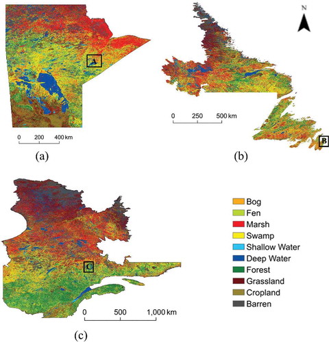
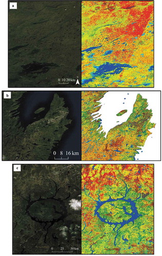
Figure 3. The zoomed imagery from the selected areas in Figure 2 (i.e. A, B, C), illustrating the visual accuracy of the produced provincial wetland inventory maps (see Figure 2 for the legend of the maps).

Table 3 provides the accuracies of the classifications obtained from the confusion matrix. The overall accuracies for Manitoba, Quebec, and NL were 84%, 78%, and 82%, respectively, indicating that the provinces were overall mapped with high accuracies considering that large areas were classified. Furthermore, the average producer and user accuracies for the five wetland classes were approximately 77% and 73% for Manitoba, 67% and 73% for Quebec, and 71% and 74% for NL, respectively. These statistics were relatively higher for non-wetland classes, for which the average producer and user accuracies were around 80%. This is because the confusion between different wetland classes is more substantial than between wetlands and non-wetlands.

Table 3. The producer and user accuracies of wetland and non-wetland classes obtained from the province-wide wetland maps at three Canadian provinces.

Wetland
	Manitoba		Quebec		NL
Class	PA (%)	UA (%)	PA (%)	UA (%)	PA (%)	UA (%)
Bog	70	63	56	62	64	72
Fen	64	59	62	78	65	66
Marsh	76	79	75	82	82	70
Swamp	83	77	65	70	64	74
Shallow Water	92	88	79	71	82	88
Average	77	73	67	73	71	74
Non-wetland
Deep Water	100	92	92	99	94	97
Forest	84	88	84	83	77	85
Grassland	87	64	68	73	55	70
Cropland	58	89	77	42	78	68
Barren	92	94	91	88	87	92
Average	84	85	82	77	78	82
Overall Accuracy (%)	84		78		82
Kapa Coefficient	0.82		0.77		0.79

NL: Newfoundland and Labrador; PA: Producer Accuracy; UA: User Accuracy.

The current research utilized a new supervised classification approach to map wetlands covering large areas (e.g. a province) without the use of field samples. The classification accuracies (Table 3) were reasonable considering the large areas that were classified and compared to the results of studies conducted over relatively smaller areas (e.g. Hird et al., 2017; Shelestov et al., 2017). The factors that hindered improvement in the level of accuracy and avenues to improve this in future studies are discussed below.

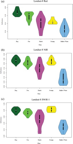
As discussed extensively in previous studies (e.g. Mahdavi et al., 2018), wetlands are spectrally similar because they share similar ecological characteristics. Therefore, distinguishing them using remote sensing datasets and machine learning algorithms is challenging and, consequently, the accuracies for wetland classes were generally lower from those of non-wetland classes. For instance, Fen, Marsh, Swamp, and Shallow Water are minerogenous wetlands, meaning that they can receive water from multiple sources, such as surface water flow and precipitation, and water can be standing or flowing. In addition, the soil type for both Bog and Fen is organic, while that of Marsh and Shallow Water is mostly mineral (Mitsch & Gosselink, 2000). These similarities in water, soil, and vegetation characteristics make the delineation of wetland challenging using remote sensing data. To illustrate this, Figure 4 demonstrates the distribution of the values of the five wetland classes obtained from the red, NIR, and SWIR-1 bands of Landsat-8 imagery using violin plots. Based on the results, wetland classes had generally similar values in these spectral bands. This demonstrates the challenges associated with discriminating wetland classes, especially those that are vegetated (i.e. Bog, Fen, Marsh, and Swamp), while Shallow Water was the most distinguishable class. Moreover, a high variance was observed for some of the classes. This was because each wetland class contains several subclasses with different spectral characteristics (e.g. the Bog class can be divided into the three subclasses of treed, shrubby, and open bog) and, thus, the within-class spectral values vary considerably. However, these spectral bands of Landsat-8 still showed potential for wetlands discrimination. For instance, Bog had a higher value in the red band (Figure 4(a)) and can be relatively distinguished from other wetlands due to its red/orange appearance (Amani et al., 2018a). Additionally, there is potential to discriminate the Marsh class from other wetland types using the NIR and SWIR-1 bands.

Figure 4. Violin plots of the wetland classes from the (a) Landsat-8 red, (b) NIR, and (c) SWIR-1 bands. These plots show the distribution shape of the field samples when multimodal distributions are present. The white dot, thick black bar in the center, and thin black line indicate the median value, interquartile range, and 95% confidence interval, respectively (NIR: Near Infrared, SWIR: Shortwave Infrared).

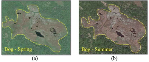
The complexity of classifying wetlands is also due to their high dynamicity; wetlands (especially Bog, Fen, and Marsh) can change significantly over time. This causes their spectral characteristics to differ between various seasons and months. For example, based on Figure 5, it is clear how the depicted Bog looks different in the spring relative to the summer and, thus, its spectral characteristics are different in satellite imagery from each season. This also illustrates the importance of multi-date satellite imagery in improving the accuracy of wetland classification.

Figure 5. A bog in (a) spring and (b) summer. Vegetation is green in summer and may be brown or absent in the early spring, fall, and winter. This illustrates how wetlands contain different spectral characteristics in satellite images at different times of the year and, thus, the importance of using multi-temporal data increases wetland classification accuracy.

A common problem in wetland mapping is that many wetlands are located in remote locations and, hence, collecting sufficient amounts of field data for these classes is difficult and costly. This work was no exception, and the fact that the study areas were considerably large exacerbates the problem. A limited amount of field samples for a class negatively influences the accuracy of its classification. Consequently, it is pivotal to increase the amount of field samples and to use more recent field datasets in order to increase the classification accuracy in future studies. For this, a collaboration among the organizations interested in preserving and monitoring wetlands is necessary. Moreover, there is a need to collect and increase the amount of non-wetland field samples to obtain reliable provincial wetland maps.

The other reason for the low classification accuracies was that the boundaries of classes, especially those of the non-wetland classes, were delineated using visual interpretation of high spatial resolution imagery rather than field observations. Consequently, the boundaries between some of the field sample classes may have been improperly delineated. For example, it is not always possible to visually define the boundary between Shallow Water and Deep Water regions and it was challenging to identify Shallow Water boundaries within large water bodies. Similarly, boundary delineation for wetland samples is difficult because wetlands do not have deterministic boundaries, but instead, occur on a continuous gradient (Zoltai & Vitt, 1995). This also explains why fuzzy classification approaches might be more appropriate for wetland mapping.

It has been suggested that more image-driven features be included in the classification to improve accuracy. For instance, texture information extracted from satellite imagery can provide the user with valuable information regarding wetlands (Durieux, Kropáček, De Grandi, & Achard, 2007; Powers, Hay, & Chen, 2012) and may even compensate for spectral information. In this study, multi-temporal Landsat-8, Sentinel-1, and CDEM imagery (13 features in total) were used in the classification and, thus, future studies should investigate and utilize all the available datasets and corresponding features within GEE to improve the accuracy of the produced province-wide wetland maps.

Image classification approaches are generally divided into two groups: pixel-based and object-based. It is widely discussed that object-based methods result in higher classification accuracy compared to pixel-based algorithms (Reif, Frohn, Lane, & Autrey, 2009; Shiraishi, Motohka, Thapa, Watanabe, & Shimada, 2014). Thus, it is suggested to investigate the potential of object-based methods in future studies.

Although several methods to improve the classification accuracy of the province-wide wetland maps (e.g. using object-based classification methods and including more field data and satellite-derived features) have been discussed in this study, it should be noted that there are several limitations to efficiently implementing these methods within GEE. For instance, the users are limited to approximately 1 million training points, which hinders improving the accuracy. As another example, the tuning parameters of the RF algorithm, especially the number of trees, have a considerable effect on classification accuracy and generally the corresponding values should be increased by increasing the number of field samples to achieve the highest possible accuracy (Amani et al., 2017a). However, there is a limitation in using a high number of trees within GEE when the amount of field samples is high. Finally, it should be noted that the current segmentation algorithms within GEE do not contain high accuracy and, thus, there is limitation in using object-based wetland mapping (Amani et al., 2019). This is more important when producing a provincial wetland inventory map because it is challenging to apply segmentation algorithms in these large areas even within the GEE platform. Consequently, when classifying a large area, a trade-off should be considered between the complexity of the classification method and level of accuracy. Despite these limitations, the present study has demonstrated the value of classifying wetlands using multi-source data in GEE.

5. Conclusion

Although several studies have applied multi-source and multi-temporal satellite data to classify wetlands in different Canadian provinces, most were developed for small regions, and cannot be effectively used for large-scale wetland classification. The main issues with implementing a province-wide wetland inventory system are: (1) processing big geo data, because hundreds of satellite images should be efficiently processed and classified over a large area; and (2) the lack of an adequate number of field samples. Thus, this study proposed a generalized supervised classification approach to classify wetlands over large areas within the GEE platform without available field samples. The overall classification accuracies from the three Canadian provinces of Manitoba, Quebec, and NL were between 78% and 84% and the average producer and accuracies for wetland classes also varied between 67 and 77% and 73 and 74%, respectively. These levels of accuracies were reasonable considering the following facts: (1) low number of field samples, (2) low cost of the study, (3) computational efficiency of the proposed method; and (4) the large area of the provinces that were classified in this study. It is suggested that the proposed approach be used for change detection in wetlands and monitoring the amount of loss and gain over the years. However, the classification accuracy should be first increased to analyze the changes with a high accuracy. The produced map can also be used as complementary information by other scientists who generally work on wetlands and to relate the results with other environmental variables, such as carbon storage.

Acknowledgments

This project was supported by the Canada Centre for Mapping and Earth Observation of Natural Resources Canada (NRCan). Field data were collected by numerous individuals from various organizations, including Environment and Climate Change Canada (ECCC), Ducks Unlimited Canada (DUC), Northeast Avalon Atlantic Coastal Action Program, and Memorial University of Newfoundland. The authors thank all these organizations for their generous support and providing such valuable datasets. We would also like to thank Mr. Simon Ilyushchenko for his comments to improve the implementation of the method within GEE and Mr. Guido Lemoine for providing his code for Lee speckle reduction filter in GEE developers website.

Disclosure statement

No potential conflict of interest was reported by the authors.

Data availability statement

The data that support the findings of this study are available from the corresponding author, [M. A], upon reasonable request.

References

- Amani, M. (2018). Wetland inventory system for NL using satellite data (what has been done and what is the next step). Real Time Water Quality Monitoring Workshop, St. John's, NL. Retrieved from https://www.mae.gov.nl.ca/waterres/rti/rtwq/conf/2018/04_MeisamAmani.pdf
- Amani, M., Mahdavi, S., Afshar, M., Brisco, B., Huang, W., Mohammad Javad Mirzadeh, S., … Hopkinson, C. (2019). Canadian wetland inventory using Google Earth Engine: The first map and preliminary results. Remote Sensing, 11(7), 842.
- Amani, M., Salehi, B., Mahdavi, S., & Brisco, B. (2018a). Spectral analysis of wetlands using multi-source optical satellite imagery. ISPRS Journal of Photogrammetry and Remote Sensing, 144, 119–136.
- Amani, M., Salehi, B., Mahdavi, S., Brisco, B., & Shehata, M. (2018b). A multiple classifier system to improve mapping complex land covers: A case study of wetland classification using SAR data in Newfoundland, Canada. International Journal of Remote Sensing, 39(21), 7370–7383.
- Amani, M., Salehi, B., Mahdavi, S., Granger, J., & Brisco, B. (2017b). Wetland classification in Newfoundland and Labrador using multi-source SAR and optical data integration. GIScience & Remote Sensing, 54(6), 779–796.
- Amani, M., Salehi, B., Mahdavi, S., Granger, J. E., Brisco, B., & Hanson, A. (2017a). Wetland classification using multi-source and multi-temporal optical remote sensing data in Newfoundland and labrador, Canada. Canadian Journal of Remote Sensing, 43(4), 360–373.
- Bourgeau-Chavez, L. L., Riordan, K., Powell, R. B., Miller, N., & Nowels, M. (2009). Improving Wetland characterization with multi-sensor, multi-temporal SAR and optical/infrared data fusion. In G. Jedlovec (Ed.), Advances in Geoscience and Remote Sensing. IntechOpen. doi:10.5772/8327. Retrieved from https://www.intechopen.com/books/advances-in-geoscience-and-remote-sensing/improving-wetland-characterization-with-multi-sensor-multi-temporal-sar-and-optical-infrared-data-fu
- Breiman, L. (2001). Random forests. Machine Learning, 45(1), 5–32.
- Brisco, B., Li, K., Tedford, B., Charbonneau, F., Yun, S., & Murnaghan, K. (2013). Compact polarimetry assessment for rice and wetland mapping. International Journal of Remote Sensing, 34(6), 1949–1964.
- Chasmer, L., Hopkinson, C., Montgomery, J., & Petrone, R. (2016). A physically based terrain morphology and vegetation structural classification for wetlands of the Boreal Plains, Alberta, Canada. Canadian Journal of Remote Sensing, 42(5), 521–540.
- Congalton, R. G. (1991). A review of assessing the accuracy of classifications of remotely sensed data. Remote Sensing of Environment, 37(1), 35–46.
- Crist, E. P., & Cicone, R. C. (1984). A physically-based transformation of Thematic Mapper data—The TM tasseled cap. IEEE Transactions on Geoscience and Remote Sensing, (3), 256–263.
- Dabboor, M., White, L., Brisco, B., & Charbonneau, F. (2015). Change detection with compact polarimetric SAR for monitoring wetlands. Canadian Journal of Remote Sensing, 41(5), 408–417.
- Durieux, L., Kropáček, J., De Grandi, G. D., & Achard, F. (2007). Object‐oriented and textural image classification of the Siberia GBFM radar mosaic combined with MERIS imagery for continental scale land cover mapping. International Journal of Remote Sensing, 28(18), 4175–4182.
- Foga, S., Scaramuzza, P. L., Guo, S., Zhu, Z., Dilley, R. D., Jr, Beckmann, T., … Laue, B. (2017). Cloud detection algorithm comparison and validation for operational Landsat data products. Remote Sensing of Environment, 194, 379–390.
- Gorelick, N., Hancher, M., Dixon, M., Ilyushchenko, S., Thau, D., & Moore, R. (2017). Google Earth Engine: Planetary-scale geospatial analysis for everyone. Remote Sensing of Environment, 202, 18–27.
- Grenier, M., Demers, A. M., Labrecque, S., Benoit, M., Fournier, R. A., & Drolet, B. (2007). An object-based method to map wetland using RADARSAT-1 and Landsat ETM images: Test case on two sites in Quebec, Canada. Canadian Journal of Remote Sensing, 33(sup1), S28–S45.
- Henderson, F. M., & Lewis, A. J. (2008). Radar detection of wetland ecosystems: A review. International Journal of Remote Sensing, 29(20), 5809–5835.
- Hird, J. N., DeLancey, E. R., McDermid, G. J., & Kariyeva, J. (2017). Google Earth Engine, open-access satellite data, and machine learning in support of large-area probabilistic wetland mapping. Remote Sensing, 9(12), 1315.
- Huang, C., Peng, Y., Lang, M., Yeo, I. Y., & McCarty, G. (2014). Wetland inundation mapping and change monitoring using Landsat and airborne LiDAR data. Remote Sensing of Environment, 141, 231–242.
- Kumar, L., & Mutanga, O. (2018). Google Earth Engine applications since inception: Usage, trends, and potential. Remote Sensing, 10(10), 1509.
- Lee, J. S., Grunes, M. R., & De Grandi, G. (1999). Polarimetric SAR speckle filtering and its implication for classification. IEEE Transactions on Geoscience and Remote Sensing, 37(5), 2363–2373.
- Lillesand, T., Kiefer, R. W., & Chipman, J. (2015). Remote sensing and image interpretation. New York, NY: John Wiley & Sons.
- Lobell, D. B., Thau, D., Seifert, C., Engle, E., & Little, B. (2015). A scalable satellite-based crop yield mapper. Remote Sensing of Environment, 164, 324–333.
- Mahdavi, S., Salehi, B., Amani, M., Granger, J., Brisco, B., & Huang, W. (2019). A dynamic classification scheme for mapping spectrally similar classes: Application to wetland classification. International Journal of Applied Earth Observation and Geoinformation, 83, 101914.
- Mahdavi, S., Salehi, B., Amani, M., Granger, J. E., Brisco, B., Huang, W., & Hanson, A. (2017). Object-based classification of wetlands in Newfoundland and Labrador using multi-temporal PolSAR data. Canadian Journal of Remote Sensing, 43(5), 432–450.
- Mahdavi, S., Salehi, B., Granger, J., Amani, M., Brisco, B., & Huang, W. (2018). Remote sensing for wetland classification: A comprehensive review. GIScience & Remote Sensing, 55(5), 623–658.
- McAlpine, D. F., & Smith, I. M. (Eds.). (2010). Assessment of species diversity in the Atlantic maritime ecozone. Ottawa, ON: NRC Research Press.
- Mitsch, W., & Gosselink, J. (2000). Wetlands (3rd ed.). New York, USA: John Wiley & Sons, Inc.
- Mutanga, O., Adam, E., & Cho, M. A. (2012). High density biomass estimation for wetland vegetation using WorldView-2 imagery and random forest regression algorithm. International Journal of Applied Earth Observation and Geoinformation, 18, 399–406.
- NRCan, N. R. (2016). Canadian digital elevation model: Product specifications-edition 1.1. Map Information, Government of Canada, Natural Resources Canada Ottawa.
- Ozesmi, S. L., & Bauer, M. E. (2002). Satellite remote sensing of wetlands. Wetlands Ecology and Management, 10(5), 381–402.
- Pekel, J. F., Cottam, A., Gorelick, N., & Belward, A. S. (2016). High-resolution mapping of global surface water and its long-term changes. Nature, 540(7633), 418.
- Powers, R. P., Hay, G. J., & Chen, G. (2012). How wetland type and area differ through scale: A GEOBIA case study in Alberta’s Boreal Plains. Remote Sensing of Environment, 117, 135–145.
- Reif, M., Frohn, R. C., Lane, C. R., & Autrey, B. (2009). Mapping isolated wetlands in a karst landscape: GIS and remote sensing methods. GIScience & Remote Sensing, 46(2), 187–211.
- Shelestov, A., Lavreniuk, M., Kussul, N., Novikov, A., & Skakun, S. (2017). Exploring Google earth engine platform for big data processing: Classification of multi-temporal satellite imagery for crop mapping. Frontiers in Earth Science, 5, 17.
- Shiraishi, T., Motohka, T., Thapa, R. B., Watanabe, M., & Shimada, M. (2014). Comparative assessment of supervised classifiers for land use–Land cover classification in a tropical region using time-series PALSAR mosaic data. IEEE Journal of Selected Topics in Applied Earth Observations and Remote Sensing, 7(4), 1186–1199.
- Vermote, E., Justice, C., Claverie, M., & Franch, B. (2016). Preliminary analysis of the performance of the Landsat 8/OLI land surface reflectance product. Remote Sensing of Environment, 185, 46–56.
- Warner, B. G., & Rubec, C. D. A., eds. (1997). The Canadian wetland classification system. Canada Committee on Ecological (Biophysical) Land Classification, National Wetlands Working Group, Wetlands Research Branch, University of Waterloo.
- White, L., Brisco, B., Dabboor, M., Schmitt, A., & Pratt, A. (2015). A collection of SAR methodologies for monitoring wetlands. Remote Sensing, 7(6), 7615–7645.
- Whiteside, T., & Bartolo, R. (2015). Mapping aquatic vegetation in a tropical wetland using high spatial resolution multispectral satellite imagery. Remote Sensing, 7(9), 11664–11694.
- Wulder, M., Li, Z., Campbell, E., White, J., Hobart, G., Hermosilla, T., & Coops, N. (2018). A national assessment of wetland status and trends for Canada’s Forested ecosystems using 33 years of earth observation satellite data. Remote Sensing, 10(10), 1623.
- Xiong, J., Thenkabail, P. S., Gumma, M. K., Teluguntla, P., Poehnelt, J., Congalton, R. G., … Thau, D. (2017). Automated cropland mapping of continental Africa using Google Earth Engine cloud computing. ISPRS Journal of Photogrammetry and Remote Sensing, 126, 225–244.
- Zhang, Q., Li, B., Thau, D., & Moore, R. (2015). Building a better urban picture: Combining day and night remote sensing imagery. Remote Sensing, 7(9), 11887–11913.
- Zoltai, S. C., & Vitt, D. H. (1995). Canadian wetlands: Environmental gradients and classification. Vegetatio, 118(1–2), 131–137.