Daily sea ice concentration product based on brightness temperature data of FY-3D MWRI in the Arctic

ABSTRACT

A daily sea ice concentration (SIC) product in the Arctic, derived from the brightness temperature (TB) data of the Microwave Radiation Imager (MWRI) sensor aboard on the FY-3D satellite, is described in this paper. The MWRI TB raw swath data were first processed into daily gridded data and then corrected using the Advanced Microwave Scanning Radiometer 2 (AMSR2) sensor. An ASI algorithm, which uses daily dynamic tie points, was adopted to calculate daily SIC at 12.5 km polar stereographic projection from January 2018 to June 2020. Our generated MWRI SIC product was compared with the AMSR2 SIC based on the ASI algorithm that uses fixed tie points. For more detailed comparison, we then compared our MWRI SIC with the SIC from the Moderate Resolution Imaging Spectroradiometer (MODIS) data. The mean bias between our MWRI SIC and AMSR2 SIC is 4.24%. The absolute values of biases between the daily MWRI SIC and MODIS SIC range from 0.14% to 10.76%, better than the MWRI SIC product based on the NT2 algorithm published by the Chinese National Satellite Meteorological Center. The results show that our MWRI SIC product has a good quality and can be used as a basic dataset for sea ice extent records. The dataset is available at http://www.dx.doi.org/10.11922/sciencedb.00137.

KEYWORDS:

• Sea ice concentration
• FY-3D MWRI
• brightness temperature
• Arctic

1. Introduction

It is well known that sea ice plays an essential role in the climate system, regulating the heat exchange between the ocean and atmosphere (Stroeve & Notz, 2018). Most of sea ice is distributed in the polar regions with high variability. Recently, the extent and area of sea ice in the Arctic have significantly declined (Meier et al., 2014). Sea ice concentration (SIC), as a basic parameter of sea ice distribution, has been continuously obtained from passive microwave (PM) sensors for more than four decades.

There are a plenty of satellite-based PM SIC products released by different institutions. The American National Snow and Ice Data Center (NSIDC) provides SIC climate data records. One of the SIC data records published daily for the Arctic and Antarctic at 25 km grid resolution is based on the NASA Team (NT) algorithm (Cavalieri, Gloersen, & Campbell, 1984; Cavalieri, Parkinson, Gloersen, Comiso, & Zwally, 1999) and the Bootstrap (BST) algorithm (Comiso, 1986; Comiso, Cavalieri, Parkinson, & Gloersen, 1997; Comiso & Nishio, 2008), using brightness temperature (TB) data from the Special Sensor Microwave/Imager (SSM/I) and Special Sensor Microwave Imager Sounder (SSMIS) sensors. Other data records at both 12.5 km and 25 km grid resolution are produced from the Advanced Microwave Scanning Radiometer-EOS (AMSR-E) and Advanced Microwave Scanning Radiometer 2 (AMSR2) sensors, which leverage the Enhanced NASA Team (NT2) algorithm (Markus & Cavalieri, 2009, 2000) and the AMSR BST algorithm (Comiso, Cavalieri, & Markus, 2003). The Integrated Climate Data Center (ICDC) of the University of Hamburg generates the SIC product for both hemispheres since 1991 at 12.5 km grid resolution by applying the Arctic Radiation and Turbulence Interaction Study Sea Ice (ASI) algorithm (Kaleschke et al., 2001) to TB data at near-90 GHz of the SSM/I and SSMIS sensors. Another SIC product, based on the ASI algorithm at higher grid resolutions of 3.125 km and 6.25 km, is regularly published by the University of Bremen, Institute of Environmental Physics (IUP) from the AMSR-E and AMSR2 sensors (Spreen, Kaleschke, & Heygster, 2008). The European Organisation for the Exploitation of Meteorological Satellites (EUMETSAT) Ocean and Sea Ice Satellite Application Facility (OSI SAF) releases a daily climate data record (OSI-450) at 25 km grid resolution, employing a self-optimizing hybrid algorithm. This dataset combines the BST algorithm (Comiso, 1986) and a generalized Bristol (Smith, 1996) to TB data from the Scanning Multichannel Microwave Radiometer (SMMR), SSM/I, and SSMIS sensors (Lavergne et al., 2019). Two other climate data records obtained from the AMSR-E and AMSR2 data since 2002 are released by the European Space Agency (ESA) Climate Change Initiative (CCI) program at 25 km grid resolution (SICCI-25 km) and 50 km grid resolution (SICCI-50 km) (Lavergne et al., 2019).

The Microwave Radiation Imager (MWRI) sensors are developed by China aboard the FengYun-3 (FY-3) series satellites, which are second-generation sun-synchronous meteorological satellites. The MWRI sensor has been operating since it was first launched on FY-3A satellite in 2008. Currently, the MWRI sensors aboard the FY-3B, −3C and −3D satellites are all operating normally, while the FY-3A MWRI failed. The Chinese National Satellite Meteorological Center (NSMC) provides daily TB data in real-time, but the publishing of FY-3A and −3B SIC data has been discontinued. The FY-3D MWRI TB dataset has been provided since the launch of the FY-3D satellite in November 2017. The SIC products, based on the NT2 algorithm at 12.5 km grid resolution, have been generated daily by the Chinese NSMC since June 2011, using TB data from the MWRI sensors on FY-3B, −3C and −3D platforms (Wu & Liu, 2018). The newest MWRI SIC product from FY-3D for the Arctic and Antarctic has been published daily since July 2018.

Different algorithms for retrieving SIC have been employed to other sensors, such as the SSM/I, SSMIS, AMSR-E and AMSR2 sensors. However, the published SIC products of the MWRI sensors are only based on the NT2 algorithm. Providing SIC products from the same sensors using different algorithms is crucial for sea ice monitoring. The Arctic SIC product at 12.5 km grid resolution generated in this study is derived from the FY-3D MWRI sensor using an ASI algorithm involving dynamic tie points. The TB data of the FY-3D MWRI sensor were preprocessed into a daily gridded TB dataset, which was then corrected to minimize bias between the MWRI and AMSR2 TB data. The SIC was calculated from the corrected TB dataset based on an ASI dynamic tie points algorithm. Furthermore, the validation of this SIC product was performed by comparing it with the SIC retrieved from AMSR2 data and Moderate Resolution Imaging Spectroradiometer (MODIS) data.

2. Methods

2.1. Data sources

The main data source of our product is the TB data of the FY-3D MWRI sensors available from the Chinese NSMC (http://data.nsmc.org.cn). We used the FY-3D MWRI L1 data, including swath data of ascending and descending orbits. The difference between two adjacent overpass periods is 54 minutes. Within each day, around 28 swaths cover the polar region except for the Pole Hole. These data archived in HDF5 format comprising 14 scientific datasets (SDS). The primary SDS applied to calculate our SIC product is the earth observation TB data, called “EARTH_OBSERVE_BT_10_to_89 GHz”. This SDS contains 10 channels in 5 frequencies of 10.65 GHz, 18.7 GHz, 23.8 GHz, 36.5 GHz, and 89 GHz at both horizontal (H) and vertical (V) polarizations. The spatial resolution in each channel is different, ranging from 9 km at 89 GHz to 85 km at 10.65 GHz. We acquired the FY-3D MWRI L1 TB data for January 2018 to June 2020.

Another data source is the TB data of the AMSR2 sensor used to correct the bias between MWRI and AMSR2 TB data. The AMSR2 TB data are from the dataset called ‘AMSR-E/AMSR2 Unified L3 Daily 12.5 km Brightness Temperatures, Sea Ice Concentration, Motion & Snow Depth Polar Grids, Version 1ʹ archived in NSIDC (Meier, Markus, & Comiso, 2018). This TB dataset is daily gridded at 12.5 km spatial resolution at polar stereographic projection. We obtained the AMSR2 TB data for January 2018 to June 2020.

2.2. TB data processing

Before calculating SIC, we implemented a series of processing steps to get the daily gridded TB data. The geolocation was conducted based on the SDS called “Latitude” and “Longitude” using the tool – “ReprojectGLT” of Envitask – in the IDL software. The calibration was executed using the following equation:

(1) $\begin{array}{c}TB=DN\times 0.01+327.68\end{array}$(1)

where $DN$ is the pixel value stored in “EARTH_OBSERVE_BT_10_to_89 GHz”. All swaths of the TB data were projected into the NSIDC polar stereographic projection at 12.5 km resolution, with the standard latitude at 70° N. Each swath pixel of the TB data observed within one calendar day was composited into the daily gridded TB data using a drop-in-the-bucket method. We gridded the TB data of all ascending orbits and all descending orbits, respectively. The daily averaged gridded TB data were then obtained by taking the average value of the ascending and descending gridded TB data. The daily averaged gridded TB data were then used as input for the subsequent process steps.

To reduce the TB bias between the MWRI and AMSR2 sensors and retrieve highly consistent SIC for the long-term record, we corrected the MWRI TB according to the AMSR2 TB data. The correction procedure adopted in this paper is referred to Meier and Ivanoff (2017). First, we selected the TB sample pairs for the year 2018 to construct the correction models. Due to the weather influence, the variability of the ice surface, time difference in swath observations and daily gridding procedure, some spurious spatial gradients are presented on the daily gridded TB data, especially during summer, leading to a large instability in bias corrections. These daily gridded TB data affected by spatial gradients (from 23 to 26 February, 10 March, 4 and 5 April, from 9 May to 3 October, and 13 October in 2018) were excluded in the selection of TB sample pairs. The TB sample pairs were restricted in areas where the SIC of AMSR2, based on the NT2 algorithm, is larger than 15%, and the latitude of the areas is within 66.5° N to 87° N. Then, we made a linear regression analysis between two TB datasets based on TB sample pairs for each day in 2018. The daily regression coefficients were averaged over 2018 as the yearly correction model at five channels (Table 1). Finally, we applied the yearly model to correct the MWRI TB data from January 2018 to June 2020 by the following equation:

(2) $\begin{array}{c}Y=a+bX\end{array}$(2)

Table 1. The yearly models of bias correction at five channels. The bias between MWRI and AMSR2 TB data before and after bias correction from January 2018 to June 2020.

Channel	Slope	Intercept	Sea ice bias (K)		Open water bias (K)
			Before	After	Before	After
18.7 V	0.900	28.014	-4.0	-0.3	-9.7	<0.0
23.8 V	0.956	15.642	-5.3	-0.3	-9.5	-2.6
36.5 V	0.970	12.454	-6.0	-0.5	-10.0	-3.7
89 H	0.972	8.625	-2.5	0.1	-2.6	0.2
89 V	0.979	8.237	-3.5	<0.0	-4.2	-1.1

where $a$ is the intercept of yearly model (the third column in Table 1), $b$ is the slope of yearly model (the second column in Table 1), $X$ is the MWRI TB data before correction and $Y$ is the MWRI TB data after correction. After bias correction, the two TB data achieved better consistency, and results are shown in Table 1. The absolute values of sea ice biases are within 0.5 K, especially near 0 K at 89 GHz. The MWRI TB data are slightly lower than AMSR2 TB except for 89 GHz at horizontal polarization, which is slightly higher. The biases over open water have also decreased, but remain larger than over sea ice, except for 18.7 GHz at vertical polarization.

2.3. SIC Calculation

The MWRI SIC in this paper was calculated by an ASI algorithm using dynamic tie points. The ASI algorithm has been developed for the AMSR-E and AMSR2 sensors (Melsheimer, 2019; Spreen et al., 2008), which is based on the polarization differences, written as:

(3) $\begin{array}{c}P=T{B}_V-T{B}_H\end{array}$(3)

where $P$ is the polarization difference, $T{B}_V$ is the TB at vertical polarization and $T{B}_H$ is the TB at horizontal polarization. Previous research has shown that the polarization difference in all ice types is similar and much smaller than over open water at near-90 GHz (Spreen et al., 2008). The polarization difference at 89 GHz of closed ice is P₁ for SIC equal to 100%, and the polarization difference at 89 GHz of open water is P₀ for SIC equal to 0%. The P₁ and P₀ are called sea ice tie points and open water tie points, respectively. Assuming the atmospheric influence to be a smooth function of SIC, a third-order polynomial is chosen to calculate the SIC ranging from open water and 100% closed ice, given by:

(4) $\begin{array}{c}SIC=d_3{P}^3+d_2{P}^2+d_{1}P+d_0\end{array}$(4)

where $d_0$, $d_1$, $d_2$, $d_3$ are the coefficients of the polynomial. The polynomial coefficients were calculated from tie points P₁ and P₀. Assuming the polarization differences of 100% sea ice-covered and open water are known, the SIC can be calculated. See Kaleschke et al. (2001) and Spreen et al. (2008) for more details of the ASI algorithm.

According to the above algorithm principle, the initial MWRI SIC was calculated using the fixed tie points P₁ = 11.7 K and P₀ = 47 K, which were applied to the AMSR-E and AMSR2 SIC products (Melsheimer, 2019; Spreen et al., 2008). The weather filters and maximum ice extent masks were not employed in the initial SIC to reduce the weather influence in selecting dynamic tie-points samples.

Based on this initial SIC, we generated the dynamic tie points. The sea ice tie-point samples were selected from grid cells with the initial MWRI SIC greater than 95%. Since weather filters were not used to produce the initial MWRI SIC, resulting in potential spurious sea ice (SIC greater than 95%) over open water, we restrained the samples within the monthly minimum ice extent mask. To mitigate the effects on land-spillover and the unstable observations near the pole, only the samples 100 km away from the coastal regions and southern than 87° N were selected. Samples that satisfied the above four conditions were used to compute the sea ice tie points. To filter out weather-impacted grid cells over open water, we selected grid cells with the initial MWRI SIC between −10% and 10% for open water tie-point samples. At the same time, the samples have to satisfy the following requirements: between 200 km to 350 km away from the monthly maximum ice extent mask, 100 km away from coastal regions and northern than 50° N.

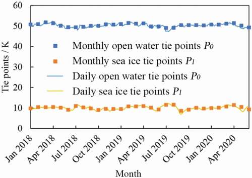
Furthermore, a central sliding window (±7 days), similar to Lavergne et al. (2019), was used to calculate the average tie points P₁ and P₀ centered at the interest day within the 15-day time window. The daily dynamic tie points and monthly averages are shown in Figure 1. The annual averages for sea ice tie points P₁ in 2018 and 2019 are 9.9 K and 10.1 K, and the yearly means for open water tie points P₀ are 50.4 K and 50.3 K, respectively.

Figure 1. The result of daily (solid curves) and monthly (solid rectangles) dynamic sea ice tie points P₁ (orange) and open water tie points P₀ (blue) from January 2018 to June 2020.

The final MWRI SIC was calculated based on the computed dynamic tie points. However, spurious sea ice over open water may exist due to variations in sea surface roughness caused by surface wind, rainfall, water vapor and cloud liquid water, which are extremely sensitive at near-90 GHz (Kern, 2004). These spurious sea ice were removed using the following filtering steps:

(5) $\begin{array}{c}GR\left(36.5/18.7\right)=\frac{T{B}_V\left(36.5\right)-T{B}_V\left(18.7\right)}{T{B}_V\left(36.5\right)+T{B}_V\left(18.7\right)}\end{array}$(5)

where $T{B}_V\left(36.5\right)$ is the TB at 36.5 GHz at vertical polarization and $T{B}_V\left(18.7\right)$ is the TB at 18.7 GHz at vertical polarization (Gloersen & Cavalieri, 1986).

(6) $\begin{array}{c}GR\left(23.8/18.7\right)=\frac{T{B}_V\left(23.8\right)-T{B}_V\left(18.7\right)}{T{B}_V\left(23.8\right)+T{B}_V\left(18.7\right)}\end{array}$(6)

where $T{B}_V\left(23.8\right)$ is the TB at 23.8 GHz at vertical polarization (Cavalieri, Germain, & Swift, 1995). We set the SIC to 0% when the value of $GR\left(36.5/18.7\right)$ was greater than 0.045 or $GR\left(23.8/18.7\right)$ exceeded 0.04 (Spreen et al., 2008). A monthly maximum ice extent mask acquired from 1979 to 2017 (Stroeve & Meier, 2018) was applied to remove the remaining spurious sea ice at low latitude, and the SIC beyond the monthly maximum ice extent was set to 0%. Our Arctic SIC product was generated daily from January 2018 to June 2020, stored in a dataset provided with this paper.

3. Data records

The dataset provided in this paper consists of two parts – the dynamic tie points and the Arctic MWRI SIC product. The dynamic tie points are stored in XLSX format, called “dynamic tie points_2018.01–2020.06.xlsx”. The first column in the file is the date, the second is sea ice tie points and the third is open water tie points. A pair of tie points is attached to each day. The Arctic MWRI SIC product is daily gridded SIC at polar stereographic projection with the spatial resolution of 12.5 km, based on an ASI algorithm employing dynamic tie points. This SIC product, acquired for January 2018 to June 2020, is in TIFF format. The naming convention of this product is “FY-3D_MWRI_SIC_DAILY_YYYYMMDD.tif”, and the meaning of the file name variables – “YYYYMMDD ” – serves as the date stamp. The pixel values in the TIFF files have specific meanings: “1–100” represents the percent of SIC, “0” is for open water, “-1” is for land, “-2” is for the Pole Hole and “NoData” means missing data. The information of our MWRI SIC product is summarized in Table 2.

Table 2. The information of the MWRI SIC product provided by this study.

Variable	Description
Naming convention	FY-3D_MWRI_SIC_DAILY_YYYYMMDD.tif
YYYY	Four-digit year
MM	Two-digit month
DD	Two-digit day
Projection	NSIDC Sea Ice Polar Stereographic North
Spatial resolution	12.5 km
Extent
Upper left point	30.98° N 168.35° E
Lower left point	33.92° N 80.74° W
Upper right point	31.37° N 102.34° E
Lower right point	34.35° N 9.97° W
Pixels values
0	Open water
1–100	Sea ice concentration
−1	Land
−2	Pole Hole
NoData	Missing data

4. Product validation

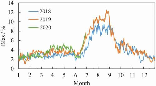
We compared the AMSR2 SIC product based on the ASI algorithm using fixed tie points with our MWRI SIC product. The AMSR2 SIC product is published by the University of Bremen (https://seaice.uni-bremen.de/). The AMSR2 SIC product has a polar stereographic projection at the 6.25 km spatial resolution. For the AMSR2 SIC product, we resampled the data to 12.5 km and employed the same land mask and Polar Hole mask used in our MWRI SIC product. The bias between our MWRI SIC and the AMSR2 SIC is presented in Figure 2. The mean bias between the two SIC products during the period of comparison is 4.24%. The bias is within 6% during winter and amplifies from early July to late September. This seasonal trend can be seen in both 2018 and 2019, although the bias in 2018 is lightly lower. The correlation between the two products is high, with an average correlation coefficient of 0.91.

Figure 2. The bias between our MWRI SIC product and AMSR2 SIC product based on the ASI algorithm using fixed tie points from January 2018 to June 2020.

To validate the quality of the dataset, remote sensing data with higher spatial resolution – MODIS – was used. However, the optical sensors (i.e. MODIS) are considerably affected by weather, particularly cloud contamination. Thus, validation was performed on images with clear-sky conditions. Several cloud-free MODIS scenes, located around the Arctic and acquired from April to August in 2018, were chosen for the validation analysis. The spatial distribution of the selected MODIS scenes is shown in Figure 3. The MODIS data used in the validation procedure are Band 2 (0.841 μm – 0.876 μm) of the MOD02QKM at 250 m spatial resolution (MODIS Characterization Support Team (MCST), 2017). Processing was conducted using ENVI software, which includes calibrating radiation, removing the Bow-Tie effect, and correcting geolocations. The obtained reflectance data were projected at polar stereographic grid, comparable with the MWRI SIC. We then used the cloud mask from the MOD35 product to remove cloud-covered areas, clipping the images into a cloud-free subset. Based on the Otsu method (Otsu, 1979), a threshold strategy that uses the image’s grey-level histogram to maximize the variances between two classes was applied for the binary classification. Each pixel was classified either as ice or water using Band 2 reflectance threshold in Table 3. Based on the ice-water binary map, we computed the ratio of ice pixels to the total number of pixels at 12.5 km grid resolution to generate the MODIS SIC.

Figure 3. The spatial distribution of MODIS scenes used in this study.

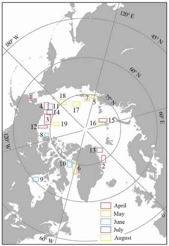
Table 3. The validation results of the MWRI SIC with the MODIS SIC in 2018.

No.	Date	Threshold	N	Bias (%)	RMSD (%)	R
1	02 April	0.17	225	−0.16	20.97	0.81
2	13 April	0.11	390	−0.14	8.82	0.96
3	15 April	0.13	814	−0.84	3.85	0.25
4	19 April	0.12	432	0.41	16.93	0.90
5	04 May	0.11	308	−2.17	7.29	0.91
6	12 May	0.13	598	2.07	8.50	0.70
7	25 May	0.11	315	−4.09	16.03	0.84
8	02 June	0.11	156	−2.40	12.93	0.92
9	08 June	0.16	320	−2.96	8.18	0.99
10	15 June	0.18	442	−5.22	12.00	0.96
11	26 June	0.04	437	−5.41	18.63	0.90
12	02 July	0.12	297	−4.76	12.12	0.96
13	13 July	0.14	320	−10.59	16.82	0.91
14	14 July	0.05	380	−8.38	16.42	0.91
15	22 July	0.07	390	1.83	12.34	0.95
16	02 August	0.09	192	10.76	17.35	0.94
17	06 August	0.09	378	0.93	16.59	0.81
18	13 August	0.11	456	−2.90	18.40	0.79
19	24 August	0.11	297	−4.74	11.74	0.95

Note; N is the number of compared pixels at 12.5 km resolution, “RMSD” is the root mean square deviation, “R” is correlation coefficients.

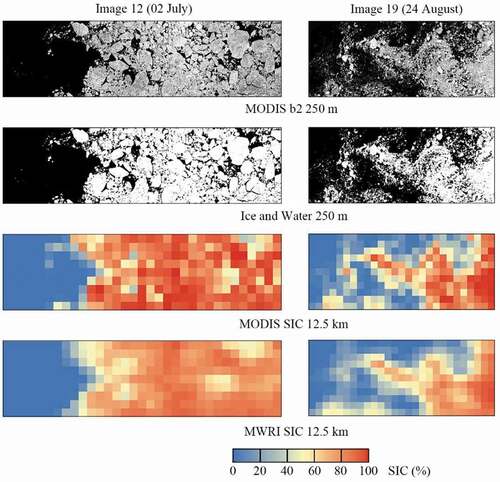
We then compared our MWRI SIC with the MODIS SIC, and the comparison results are shown in Table 3. Several images are presented in Figures 4–7, including the reflectance of Band 2, the ice-water binary map, the MODIS SIC, and the MWRI SIC. From Table 3, the absolute values of bias range from 0.14% to 10.76%. The RMSDs in 18 images are lower than 20%, while the maximum RMSD is 20.97%. In 13 out of the 19 images, the correlation coefficients are larger than 0.9. Image 6 has a low correlation coefficient with the value of 0.7 due to the presence of leads in this image (Figure 4). Passive microwave sensors are weaker in identifying leads than optical sensors that have much higher resolution. For instance, Image 3 (Figure 5) shows a distribution with thinner leads, resulting in a 0.25 correlation, a negative 0.84% bias, and a 3.85% RMSD. For melting areas, as shown in Image 1 (Figure 4) and Image 7 (Figure 5), the correlation is also low 0.81 for Image 1 and 0.84 for Image 7. The highest correlation coefficient (0.99) and the low RMSD (8.18%) were observed in Image 9 (Figure 6), which is located at compact ice edges. In diffuse ice edge, although the correlation coefficient is higher than 0.9, there are larger bias and RMSD values than compact ice edge area, as shown in Image 10 (Figure 5), Image 12 (Figure 7) and Image 19 (Figure 7). Note that the SIC in pack ice was underestimated by our MWRI SIC.

Figure 4. MODIS Band 2 reflectance, the ice-water binary map, the MODIS SIC, and the MWRI SIC of Image 1 (02 April 2018) and Image 6 (12 May 2018).

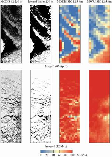
Figure 5. MODIS Band 2 reflectance, the ice-water binary map, the MODIS SIC, and the MWRI SIC of Image 3 (15 April 2018), Image 7 (25 May 2018) and Image 10 (15 June 2018).

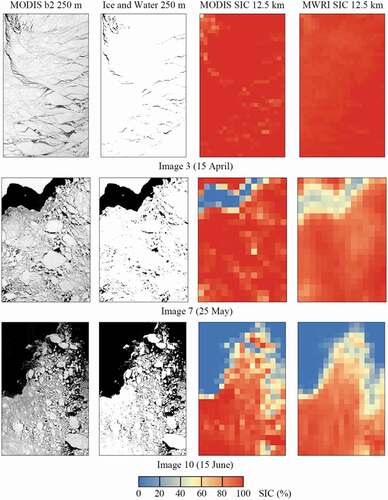
Figure 6. MODIS Band 2 reflectance, the ice-water binary map, the MODIS SIC, and the MWRI SIC of Image 9 (08 June 2018), Image 14 (14 July 2018) and Image 16 (02 August 2018).

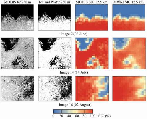
Figure 7. MODIS Band 2 reflectance, the ice-water binary map, the MODIS SIC, and the MWRI SIC of Image 12 (02 July 2018) and Image 19 (24 August 2018).

5. Data set value

Previous studies have shown that inter-instrument biases and error sources with climatological trends can be largely reduced by using seasonal tie points (Ivanova et al., 2015). Hao and Su (2015) have shown that the SIC obtained from AMSR-E data based on an ASI algorithm using dynamic tie points provides better results than that using fixed tie points. Daily dynamic tie points were considered to our SIC product.

The published FY-3D MWRI SIC product based on the NT2 algorithm, using the same spatial resolution as our SIC product, is available from the Chinese NSMC starting 12 July 2018. Seven MODIS images in July and August 2018 corresponding to the published MWRI SIC product were used in this study. We compared the published MWRI SIC to MODIS SIC, and the results are shown in Table 4. The biases are higher than 15%, with some as large as 30.51%, except for Image 14 (0.59%) and Image 15 (10.83%). The RMSDs all exceed 18%, with one even reaching 39.39%. In term of correlation coefficient, all images have values lower than 0.8, except for Image 15, which has 0.93; for Image 18, the value is as low as 0.47. From the statistic validation analysis, we found that our SIC product performed better than the published MWRI SIC product based on the NT2 algorithm. Our generated product also has a great potential for analysing the long-term sea ice area and sea ice extent, which can be useful for global climate change studies.

Table 4. The comparison results between two MWRI SICs and the corresponding MODIS SIC in 2018. “A/B”: A is the statistic results of our MWRI SIC product and B is the statistic results of the published MWRI SIC product based on the NT2 algorithm.

No.	Date	Bias (%)	RMSD (%)	R
13	13 July	−10.59/30.51	16.82/39.39	0.91/0.64
14	14 July	−8.38/0.59	16.42/21.43	0.91/0.77
15	22 July	1.83/10.83	12.34/18.83	0.95/0.93
16	02 August	10.76/19.48	17.35/30.64	0.94/0.76
17	06 August	0.93/22.10	16.59/31.97	0.81/0.63
18	13 August	−2.90/25.51	18.40/36.20	0.79/0.47
19	24 August	−4.74/26.10	11.74/35.40	0.95/0.69

Acknowledgments

The research presented in this paper is funded by the National Key Research and Development Program of China (2018YFC1407100) and the National Natural Science Foundation of China (41876223). The authors are grateful to the Chinese National Satellite Meteorological Center for providing MWRI datasets, the US Geological Survey (USGS), NASA National Snow and Ice Data Center and Goddard Space Flight Center for providing AMSR2 and MODIS datasets, the University of Bremen, Institute of Environmental Physics for providing AMSR2 SIC product. We would like to thank Dr. Shengli Wu, who is working at the Chinese National Satellite Meteorological Center, for his good communications.

Data Availability Statement

The dataset is openly available in the Science Data Bank at http://www.dx.doi.org/10.11922/sciencedb.00137.

Disclosure statement

No potential conflict of interest was reported by the authors.

Additional information

Funding

This work was supported by the National Key Research and Development Program of China [2018YFC1407100] and the National Natural Science Foundation of China [41876223].

Notes on contributors

Xi Zhao

Xi Zhao is an Associate Professor in Chinese Antarctic Center of Surveying and Mapping at Wuhan University. She received her Ph.D. in Earth Observation Science from the Faculty of Geo-Information Science and Earth Observation (ITC) at the University of Twente in the Netherlands. After her PhD research, she worked on remote sensing and uncertainty of the polar sea ice. Xi won the James Smith Medal for 2018, awarded by the International Spatial Accuracy Research Association, for her achievement as a junior scientist. She also served as a guest editor for Spatial Statistics’ special issue in 2017, and was a keynote speaker at the Spatial Statistics Conference in 2015, and again in 2018. Xi has also published over 50 peer-reviewed papers, among which 31 are SCI/EI indexed.

References

- Cavalieri, D. J., Germain, K. M. S., & Swift, C. T. (1995). Reduction of weather effects in the calculation of sea-ice concentration with the DMSP SSM/I. Journal of Glaciology, 41(139), 455–464.
- Cavalieri, D. J., Gloersen, P., & Campbell, W. J. (1984). Determination of sea ice parameters with the NIMBUS 7 SMMR. Journal of Geophysical Research, 89(D4), 5355–5369.
- Cavalieri, D. J., Parkinson, C. L., Gloersen, P., Comiso, J. C., & Zwally, H. J. (1999). Deriving long-term time series of sea ice cover from satellite passive-microwave multisensor data sets. Journal of Geophysical Research, 104(C7), 15803–15814.
- Comiso, J. C. (1986). Characteristics of Arctic winter sea ice from satellite multispectral microwave observations. Journal of Geophysical Research, 91(C1), 975–994.
- Comiso, J. C., Cavalieri, D. J., & Markus, T. (2003). Sea ice concentration, ice temperature, and snow depth using AMSR-E data. IEEE Transactions on Geoscience and Remote Sensing, 41(2), 243–252.
- Comiso, J. C., Cavalieri, D. J., Parkinson, C. L., & Gloersen, P. (1997). Passive microwave algorithms for sea ice concentration: A comparison of two techniques. Remote Sensing of Environment, 60(3), 357–384.
- Comiso, J. C., & Nishio, F. (2008). Trends in the sea ice cover using enhanced and compatible AMSR‐E, SSM/ I, and SMMR data. Journal of Geophysical Research: Oceans, 113(C2). doi:https://doi.org/10.1029/2007JC004257
- Gloersen, P., & Cavalieri, D. J. (1986). Reduction of weather effects in the calculation of sea ice concentration from microwave radiances. Journal of Geophysical Research: Oceans, 91(C3), 3913–3919.
- Hao, G., & Su, J. (2015). A study on the dynamic tie points ASI algorithm in the Arctic Ocean. Acta Oceanologica Sinica, 34(11), 126–135.
- Ivanova, N., Pedersen, L. T., Tonboe, R., Kern, S., Heygster, G., Lavergne, T., … Brucker, L. (2015). Inter-comparison and evaluation of sea ice algorithms: Towards further identification of challenges and optimal approach using passive microwave observations. The Cryosphere, 9(5), 1797–1817.
- Kaleschke, L., Lupkes, C., Vihma, T., Haarpaintner, J., Bochert, A., Hartmann, J., & Heygster, G. (2001). SSM/I sea ice remote sensing for mesoscale ocean-atmosphere interaction analysis. Canadian Journal of Remote Sensing, 27(5), 526–537.
- Kern, S. (2004). A new method for medium-resolution sea ice analysis using weather-influence corrected special sensor microwave/imager 85 GHz data. International Journal of Remote Sensing, 25(21), 4555–4582.
- Lavergne, T., Sorensen, A., Kern, S., Tonboe, R., Notz, D., Aaboe, S., … Gabarro, C. (2019). Version 2 of the EUMETSAT OSI SAF and ESA CCI sea-ice concentration climate data records. The Cryosphere, 13(1), 49–78.
- Markus, T., & Cavalieri, D. J. (2000). An enhancement of the NASA Team sea ice algorithm. IEEE Transactions on Geoscience and Remote Sensing, 38(3), 1387–1398.
- Markus, T., & Cavalieri, D. J. (2009). The AMSR-E NT2 sea ice concentration algorithm: Its basis and implementation. Journal of the Remote Sensing Society of Japan, 29, 216–225.
- Meier, W. N., Hovelsrud, G. K., Van Oort, B., Key, J. R., Kovacs, K. M., Michel, C., … Perovich, D. K. (2014). Arctic sea ice in transformation: A review of recent observed changes and impacts on biology and human activity. Reviews of Geophysics, 52(3), 185–217.
- Meier, W. N., & Ivanoff, A. (2017). Intercalibration of AMSR2 NASA Team 2 algorithm sea ice concentrations with AMSR-E slow rotation data. IEEE Journal of Selected Topics in Applied Earth Observations and Remote Sensing, 10(9), 3923–3933.
- Meier, W. N., Markus, T., & Comiso, J. C. (2018). AMSR-E/AMSR2 unified L3 daily 12.5 km brightness temperatures, sea ice concentration, motion & snow depth polar grids, Version 1. Boulder, Colorado USA: NASA National Snow and Ice Data Center Distributed Active Archive Center. doi:https://doi.org/10.5067/RA1MIJOYPK3P.
- Melsheimer, C. (2019). ASI version 5 sea ice concentration user guide. Bremen, Germany: University of Bremen, Institute of Environmental Physics.
- MODIS Characterization Support Team (MCST). (2017). MODIS 250m calibrated radiances product. USA, NASA MODIS Adaptive Processing System, Goddard Space Flight Center. doi:https://doi.org/10.5067/MODIS/MOD02QKM.061.
- Otsu, N. (1979). A threshold selection method from gray-level histograms. IEEE Transactions on Systems, Man, and Cybernetics, 9(1), 62–66.
- Smith, D. M. (1996). Extraction of winter total sea-ice concentration in the Greenland and Barents Seas from SSM/I data. International Journal of Remote Sensing, 17(13), 2625–2646.
- Spreen, G., Kaleschke, L., & Heygster, G. (2008). Sea ice remote sensing using AMSR‐E 89‐GHz channels. Journal of Geophysical Research: Oceans, 113(C2). doi:https://doi.org/10.1029/2005JC003384
- Stroeve, J., & Meier, W. N. (2018). Sea ice trends and climatologies from SMMR and SSM/I-SSMIS, version 3. Boulder, Colorado USA: NASA National Snow and Ice Data Center Distributed Active Archive Center. doi:https://doi.org/10.5067/IJ0T7HFHB9Y6.
- Stroeve, J., & Notz, D. (2018). Changing state of Arctic sea ice across all seasons. Environmental Research Letters, 13(10), 103001.
- Wu, S., & Liu, J. (2018). Comparison of Arctic sea ice concentration datasets. Haiyang Xuebao, 40, 64–72.