A satellite-derived, ground-measurement-independent monthly PM_2.5 mass concentration dataset over China during 2000–2015

ABSTRACT

Following the accelerated development of urbanization and industrialization, atmospheric particulate matter has become a significant threat to public health globally. Environmental health studies usually use the mass concentration of fine particles (PM_2.5) as a base data to predict the health risks of particulate exposure. However, PM_2.5 data from ground monitoring stations in China has not been provided until January 2013 by the Ministry of Environmental Protection of China. Hence, an alternative dataset of PM_2.5 spatiotemporal distributions extending to years earlier than 2013 is urgently needed, which is of great significance to atmospheric environment assessment and pollution prevention and control. Atmospheric aerosol products by the moderate-resolution imaging spectroradiometer (MODIS) have been released since 2000, which provides the possibility to reconstruct historical PM_2.5. However, most current methods do not have the ability to estimate PM_2.5 mass concentration independently of ground observations. The PM_2.5 mass concentration data set produced by PM_2.5 remote sensing (PMRS) model based on physical processes does not depend on the ground observations, and also is not affected by the uncertainty of model emission sources or the completeness of chemical reaction mechanism. These ensure that the point-by-point validation for PM_2.5 mass concentration data is more convincing, and the dataset can also be further used for model assimilation and artificial intelligence training to improve their predictions. In this study, we calculate the monthly PM_2.5 mass concentration near the ground over land of China using aerosol inversion products (aerosol optical depth and fine-mode fraction) of MODIS and meteorological data (boundary layer height & relative humidity) provided by the Modern-Era Retrospective Analysis for Research and Applications Version 2 (MERRA-2) data set. The results show that, in China, 6 pollution centers mainly concentrated in the central and eastern regions. The highest PM_2.5 mass concentration occurred in winter, whereas the pollution range was larger in summer. There are 63.4% of validation sites with biases within ±20 μg m⁻³, and the expected error is as ±(15 μg m⁻³ + 30%) enveloped by the monthly mean PM_2.5 mass concentrations. The monthly PM_2.5 is stored as NETCDF format, with a spatial resolution of 1°×1°. The published data is available in http://www.dx.doi.org/10.11922/sciencedb.j00076.00061.

KEYWORDS:

• PM_2.5
• data set
• satellite-derived
• China
• monthly

1. Introduction

As the pollution of fine particulate matter (PM_2.5) in the atmosphere becomes more and more serious, the harm to human health is becoming increasingly apparent. Due to an increasing number of multidisciplinary researches on pollution prevention and human exposure, the demand of PM_2.5 products is increasing. Satellite remote sensing, as a new technology, has the advantages of widely spatial coverage and strong objectivity for particle monitoring. In the past 20 years, satellite remote sensing estimation of PM_2.5 has gone through three major stages of continuous exploration, thus forming three mainstream algorithms, namely physical formula, multivariate statistical regression, and satellite-model coupling methods.

Immediately after the moderate-resolution imaging spectroradiometer (MODIS) sensor was launched into the space, validation of its aerosol products using the aerosol robotic network (AERONET) observation began. With the advancement of validation, Chu et al. (2003) found that daily average AOD from AERONET had a good correlation with 24-hour averaged PM₁₀. If the particle vertical profile was available, the inversion of atmospheric particles concentration from satellite remote sensing would become possible. In the same year, Wang and Christopher (2003) evaluated the correlation between AOD from MODIS and PM_2.5 from United States Environmental Protection Agency (EPA). They pointed out that despite the influence of ambient humidity and aerosol layer height, AOD and PM_2.5 still showed a good correlation. These two studies jointly pointed out that the aerosol optical information retrieved by satellite remote sensing can be expected to be used to estimate the particulate mass concentration near ground. Therefore, a direct linear correlation between AOD and atmospheric particulate matter was established using a basic statistical regression method. The accuracy of the estimated particle mass concentration obtained by this method is limited. Engel-Cox, Holloman, Coutant, and Hoff (2004) used MODIS satellite observations to analyze the correlation between AOD and PM_2.5 over the United States. They found that the correlation strongly depended on the temporal and spatial changes and was also related to aerosol types. Further research showed that the correlation between PM_2.5 and AOD integrated by lidar in the boundary layer was better than that with the entire atmospheric AOD (Engel-Cox et al., 2006), indicating that the aerosol vertical distribution has an important influence on this correlation. Gupta et al. (2006) evaluated the correlation between AOD and particulate matter in typical sites in Europe, the United States, and Asia. They reported that this correlation was not only affected by vertical distribution but also by ambient humidity.

However, the above methods still remain as simple statistical models until Koelemeijer, Homan, and Matthijsen (2006) first proposed a more complete theoretical derivation, which laid the foundation for the physical method of remote sensing of particulate matter. Although Koelemeijer et al. (2006) obtained a formula to calculate particulate mass concentration, it cannot yet be used to estimate the near-ground particle concentration directly. It is because even though the vertical distribution, hygroscopic growth and effective density of particulate matter can be solved by appropriate model assumptions, there is still an unknown parameter (called S hereafter) related to the particle characteristics (particle size distribution, complex refractive index, etc.), which makes it impossible for physical model to directly estimate near-ground particulate matter. This is also an important reason for giving up physical methods and the rapid development of other methods.

The statistics method, represented by the research of Liu, Paciorek, and Koutrakis (2009), has been widely used in remote sensing estimation of particulate matter near the ground. They estimated PM_2.5 mass concentration through a two-stage model using AOD, in-situ PM_2.5 and a series of auxiliary data. Other popular statistical methods (Brokamp, Jandarov, Hossain, & Ryan, 2018; Fang, Zou, Liu, Sternberg, & Zhai, 2016; He & Huang, 2018; Hu et al., 2017; Ma, Hu, Huang, Bi, & Liu, 2014; Ma et al., 2016; Shen, Li, Yuan, & Zhang, 2018; Wei et al., 2019) also included mixed effects models, random forest models, and deep learning, etc. A major advantage of these methods is that the models are directly constrained by ground observations so the uncertainty of the estimated particle mass concentration can be greatly reduced. However, it is impossible to analyze the reasons of outliers due to weakening the physical meaning of parameters in statistics method. Furthermore, statistical models unfortunately do not work so well in the areas where ground observations are sparse.

Another typical method is the combination of atmospheric chemistry transport model and satellite remote sensing as represented by Van Donkelaar et al. (2010, 2006, 2012, 2015). This method has a great advantage when estimating the spatial distribution of PM_2.5 with interannual variation, which is related to the prediction robustness of the model on a long-term scale. This method is limited by the chemistry scheme and emission inventory, and the accuracy is relatively low on a short term (daily or instantaneous observations).

Although the earlier physical methods have significant defects, there are still a few scholars who have studied them in depth. Raut and Chazette (2009) and Raut, Chazette, and Fortain (2009) calculated the unknow parameter S based on mobile lidar observations, and they also took the influence of aerosol vertical distribution and hygroscopic characteristics into account. However, this method was only developed for the wavelength of 355 nm and the type of aerosol needed to be manually set up, which had become an obstacle to its application. Kokhanovsky, Prikhach, Katsev, and Zege (2009) put forward the use of Ångström index (AE) to parameterize the effective radius of particles to solve the problem of the unknown parameter S. However, the parameterized relationship of the aerosol effective radius was established only using a single typical aerosol model, which reduced the spatiotemporal universality of their method. Subsequently, some scholars (Li et al., 2015; Lin et al., 2015; Wang, Xu, Spurr, Wang, & Drury, 2010b) obtained the spatial distribution of S within a certain period, which cannot be easily extended outside the period. Zhang and Li (2015) combined the advantages of the methods of Raut et al. (2009) and Kokhanovsky et al. (2009) and established a semi-empirical physical model, in which the volume extinction ratio (VE_f) parameter was parameterized by the fine-mode fraction (FMF) to quantify S for various typical aerosol models. And then, Zhang et al. (2020) developed a regional hygroscopic growth function so as to obtain the hygroscopicity of particulate matter with different aerosol types. This method can quickly obtain the PM_2.5 mass concentration near the ground with acceptable accuracy (Li et al., 2016), which is suitable for satellite remote sensing. The semi-empirical physical model also has disadvantages: the uncertainty of aerosol vertical distribution limits the accuracy of PM_2.5 estimates; it is difficult to control the propagation error due to the combination of multiple correction schemes.

At present, Van Donkelaar, Martin, Li, and Burnett (2019) and Wei et al. (2019) have released PM_2.5 data set generated by a chemical transport model based on Geos-Chem (http://fizz.phys.dal.ca/~atmos/martin/?page_id=140) and random forest algorithm (https://doi.org/10.5281/zenodo.3753614), respectively. Both data sets show the annual PM_2.5 mass concentrations. The former can describe the distribution of PM_2.5 at the global scale well, but the accuracy is relatively low in urban areas, while the latter is the opposite. In this research, a monthly PM_2.5 data set in China based on satellite remote sensing is produced using the semi-empirical physical method developed by Zhang and Li (2015), expecting to obtain a reasonable data set at all scales.

2. Methodology and input data

2.1. The PM_2.5 Remote Sensing (PMRS) model

In this study, we used the PMRS model (Zhang & Li, 2015) to establish a long-term data set of PM_2.5 mass concentration. The model aims to bridge the gap between remote sensing and PM_2.5 observation. PM_2.5 is defined as mass concentration of dry particles near the ground with aerodynamic diameter less than 2.5 μm, but aerosol optical depth (AOD) from remote sensing describes the sum extinction of ambient particles in columnar atmosphere. To fill this gap in-between, a series of corrections need to be performed. Firstly, AOD_f, the contribution of fine particle to AOD, is obtained by the fine mode fraction (FMF) following:

(1) $AO{D}_f=AOD\times FMF$(1)

where, fine mode fraction FMF is the ratio of AOD_f to AOD and the subscript f denotes fine mode particles. Next, we define a columnar volume-to-extinction ratio of fine particulates (VE_f) to convert AOD_f to columnar fine particle volume V_f,column:

(2) $V{E}_f=\frac{V_{f,column}}{AO{D}_f}$(2)

where, VE_f is the key parameter to link columnar optical parameters with particle microphysical properties (i.e. volume), with a unit of μm³/μm² considering particle volume in the atmospheric column is with unit of μm³/μm² and AOD_f has no unit. Further, aerosol particles generally distribute in the aerosol layer near the surface. The columnar fine particle volume can be represented by the following formula:

(3) $V_{f,column}=\underset{z_0}{\overset{H+z_0}{\int }}\underset{0}{\overset{f}{\int }}\frac{4}{3}\pi r^{3}n\left(r,z\right)drdz$(3)

where, n(r, z) is the number concentration of ambient particles. In order to deal with the vertical distribution of aerosol particles from ground (z₀, the ground altitude above sea level in unit of km) to the top of aerosol layer (H+ z₀), the vertical profile can be normalized by the particle concentration near the ground n(r, z₀) written as g’(z). The columnar fine particle volume can be deformed to

(4) $V_{f,column}=\underset{z_0}{\overset{H+z_0}{\int }}{g}^{\prime }\left(z\right)dz\underset{0}{\overset{f}{\int }}\frac{4}{3}\pi r^{3}n\left(r,z_0\right)dr$(4)

Taking the vertical integral within the aerosol layer and we can write it as below:

(5) $g\left(H\right)=\underset{z_0}{\overset{H+z_0}{\int }}{g}^{\prime }\left(z\right)dz$(5)

Following the vertical integral (Eq. (5(5) $g\left(H\right)=\underset{z_0}{\overset{H+z_0}{\int }}{g}^{\prime }\left(z\right)dz$(5) )) in Eq. (4(4) $V_{f,column}=\underset{z_0}{\overset{H+z_0}{\int }}{g}^{\prime }\left(z\right)dz\underset{0}{\overset{f}{\int }}\frac{4}{3}\pi r^{3}n\left(r,z_0\right)dr$(4) ), it yields

(6) $V_{f,column}=V_f\times g\left(H\right)$(6)

where, V_f is defined as the fine particle volume (i.e. $\underset{0}{\overset{f}{\int }}\frac{4}{3}\pi r^{3}n\left(r,z_0\right)dr$) on the ground. Since a drying process is in the sampling of fine particles near the ground, f(RH) is used to characterize the hygroscopic properties of ambient particles:

(7) $f\left(RH\right)=\frac{V_f}{V_{f,dry}}$(7)

where, V_f,dry is dry volume of fine particles near the ground and RH is the relative humidity. Finally, PM_2.5 mass concentration can be obtained by:

(8) $P{M}_{2.5}=V_{f,dry}\times {\rho }_{f,dry}$(8)

where, ρ_f,dry is the effective density of dry particles in fine mode near the ground (g cm⁻¹). By combing Eqs. (1)(1) $AO{D}_f=AOD\times FMF$(1) -(8(8) $P{M}_{2.5}=V_{f,dry}\times {\rho }_{f,dry}$(8) ), the final formula on PM_2.5 can be expressed as the product of remote sensing parameters and correction terms:

(9) $P{M}_{2.5}=AOD\frac{FMF\times V{E}_f\times {\rho }_{f,dry}}{g\left(H\right)\times f\left(RH\right)}$(9)

It should be noted that the PM_2.5 mass concentration calculated by Eq. (9)(9) $P{M}_{2.5}=AOD\frac{FMF\times V{E}_f\times {\rho }_{f,dry}}{g\left(H\right)\times f\left(RH\right)}$(9) is in unit of mg m⁻³ following the above parameter units, which needs to be multiplied by 10⁻³ to be compared with in situ measurements (unit conversion to μg m⁻³).

2.2. Columnar volume-to-extinction ratio in fine mode

VE_f defined in the previous section, has a good sensitivity to FMF, and changes monotonically with diverse aerosol types. Zhang and Li (2015) chose long-term observation for 4 typical aerosol types to parameterize the VE_f, including urban/industrial, biomass burning, dust, and sea salt type:

(10) $V{E}_f=0.2887FM{F}^2-0.4663FMF+0.356\left(0.1\le FMF\le 1.0\right)$(10)

This parameterization formula has to be restrained by FMF between 0.1 and 1.0 due to the valid sample range and lower accuracy of FMF and VE_f when FMF is less than 0.1.

2.3. Normalized vertical distribution

In polluted days, atmospheric particulate matters usually concentrate towards the ground layer and decrease sharply in the upper layer, while the particle vertical profile in clean days commonly shows a negative exponential distribution. Therefore, these two models are used to characterize the normalized vertical distribution profile of PM_2.5, namely the vertical uniform and the negative exponential models.

The vertical uniform model (Figure 1a) is the simplest one of the normalized profile models of PM_2.5 and describes a fully mixed state of PM_2.5 in the aerosol layer. In this model, there is no significant particulate matter above the aerosol layer. Therefore, we can simply assume that the vertical uniform model is

(11) $g^{\prime }\left(z\right)=\left\{\begin{array}{c}1z_0\le z\le H\\ 0z>H\end{array}\right.$(11)

We can deduce from vertical uniform model that PM_2.5 near the ground are approximately inversely proportional to the aerosol layer height, which is in agreement with Koelemeijer et al. (2006). When z₀ is the ground height (z₀ = 0), the integral of the vertical uniform model can be expressed as:

(12) $g\left(H\right)=\underset{0}{\overset{\mathrm{\infty }}{\int }}{g}^{\prime }\left(z\right)dz=\underset{0}{\overset{H}{\int }}dz=H$(12)

Figure 1. Vertical profile diagram of atmospheric particulate normalized model: (a) vertical uniform model; (b) negative exponential model.

The negative exponential model (Figure 1b) is a distribution in which the PM_2.5 concentration decreases with the aerosol layer height. The height where the concentration of the near-surface PM_2.5 decreases to 1/e is defined as the scale height (SH) of particles. Thus, the negative exponential model can be written as:

(13) $g^{\prime }\left(z\right)=e^{-\frac{z}{SH}}$(13)

Integrating Eq (13(13) $g^{\prime }\left(z\right)=e^{-\frac{z}{SH}}$(13) ), it yields:

(14) $g\left(SH\right)=\underset{0}{\overset{\mathrm{\infty }}{\int }}{e}^{-\frac{z}{SH}}dz=-SH\times \left(e^{-\mathrm{\infty }}-e^0\right)=SH$(14)

Similar to the vertical uniform model, the right side of integrated form (Eq. 14)(14) $g\left(SH\right)=\underset{0}{\overset{\mathrm{\infty }}{\int }}{e}^{-\frac{z}{SH}}dz=-SH\times \left(e^{-\mathrm{\infty }}-e^0\right)=SH$(14) is also only the height. Therefore, the integral of the normalized models can be used uniformly:

(15) $g\left(H\right)=H$(15)

When H is the aerosol layer height, the normalized model corresponds to the vertical uniform model; when H is the scale height, the normalized model corresponds to the negative exponential model. It’s worth noting that about 37% of atmospheric particles are located above the aerosol layer when atmospheric particles distribute according to the negative exponential model.

Some studies (Li et al., 2015; Lin et al., 2015; Zhang & Li, 2015) put the planet boundary layer height (PBLH) into the estimation of PM_2.5 mass concentration to replace the aerosol layer height or scale height. Although such treatment can introduce an uncertainty in a certain degree, it is also an approach that can effectively extend the aerosol vertical profile. Therefore, driven by the same parameter, the aerosol vertical model can represent two different profiles.

In addition to the above two distributions, there are other types of vertical aerosol distribution, such as a model which assumes the aerosols are well-mixed within the boundary layer and exponentially decrease in the free-atmosphere. These models often need some hard-to-observe parameters (e.g. the height of the aerosol haze layer directly observed by lidar). Thus, these vertical models are not considered in this study. Although using only two types of vertical distribution as shown in Figure 1 can introduce a certain error, the error of PM_2.5 mass concentration is within a tolerable range (Wei et al., 2021).

2.4. Hygroscopic growth function

Because the particle hygroscopicity varies greatly in different regions, a hygroscopic growth function which can characterize many types of aerosol is needed. For this purpose, the hygroscopic growth factor is reconstructed using the hygroscopic parameter (κ) to improve the performance on the spatial distribution of hygroscopic growth (Zhang et al., 2020). According to κ-Köhler theory proposed by Petters and Kreidenweis (2007), f(RH) in Equation (9)(9) $P{M}_{2.5}=AOD\frac{FMF\times V{E}_f\times {\rho }_{f,dry}}{g\left(H\right)\times f\left(RH\right)}$(9) can be derived as follows:

(16) $f\left(RH\right)=\frac{V_s+V_w}{V_s}=\frac{1-\left(1-\kappa \right)RH}{1-RH}$(16)

where V_s is the volume of the dry particulate matter and V_w is the volume of the water. The hygroscopic parameter κ can be directly measured or calculated by aerosol chemical components using a simple mixing rule:

(17) $\kappa =\sum _i{v}_i{\kappa }_i$(17)

where κ_i is the hygroscopic parameter of the individual aerosol components which can be measured in the laboratory, and v_i is the dry component volume fraction. The distribution of κ over China can be obtained by ground-based measurements (e.g. Zhang et al., 2020), modeling or remote sensing.

2.5. Strength and limitation of PMRS model

The PMRS model describes the relationship between AOD and PM_2.5 based on physical processes, which does not rely on any ground observations. This advancement enables the PMRS model to avoid empirical calibration of long-term historical data, and enhances the function of historical and instantaneous PM_2.5 estimation. This also ensures that our point-by-point validation for PM_2.5 mass concentration data is more convincing. In addition, the PMRS model is simple, flexible, fast, and suitable for people who have no experience in modeling and statistics.

The MODIS monthly products are used as input data in this study in order to reduce the uncertainty, since the PMRS model is sensitive to the errors of input parameters. The MODIS monthly products (MOD08) have high accuracy but the horizontal resolution is 1°×1°. In order to maintain the accuracy of the PM_2.5 dataset, the spatial resolution is sacrificed. In the future, as the accuracy of the inversion parameters (AOD & FMF) increases, the horizontal resolution of PM_2.5 dataset produced by the PMRS model can also be improved.

2.6. Description of input data

PM_2.5 mass concentration is estimated by available MODIS (onboard Aqua & Terra satellite) data. We employ the monthly AOD and fine-mode fraction (FMF) data with 1°×1° horizontal resolution obtained from MODIS Terra and Aqua Collection 5.1 (C5.1) monthly products over China (Levy et al., 2010) derived from dark target (DT) method (https://ladsweb.modaps.eosdis.nasa.gov/search/). MODIS/Terra products are available from March 2000 and MODIS/Aqua products are available from July 2002. The data from 2013 to 2015 for both sensors is used in this study. We chose to use C5.1 product because they include FMF which is no longer available in the new versions of products like C6 and C6.1. It is noted the AOD over China from these new versions is substantially different from the C5.1 product, by up to 0.2 (De Leeuw et al., 2018). In the PMRS method, the satellite data are matched up with PBLH and RH data extracted from the Modern-Era Retrospective Analysis for Research and Applications Version 2 (MERRA-2) reanalysis data with the horizontal resolution of 2°×2.5° (https://disc.gsfc.nasa.gov/datasets?project=MERRA-2), which are assigned into the MODIS 1°×1° grid without interpolation (e.g. Inverse Distance Weighted) to prevent the rapidly changing PBLH and RH in coastal area from being smoothed.

3. Data records

The data set generated by the PMRS model is stored in NetCDF format. There are 4 variables in the data file, including PM_2.5, latitude, longitude and time. PM_2.5 is a two-dimensional floating variable, with the horizontal grid determined by a one-dimensional array of latitude and longitude, and the unit is μg m⁻³. The horizontal resolution is 1°×1°, and the range is 72.5°E-135.5°E and 17.5°N-53.5°N for the latitude and longitude grid, respectively. The time is a combination of year (4-digit) and month (2-digit), which is recorded by an integer number (e.g. March 2000 is recorded as 200003). The PM_2.5 in the data set only has estimated values over land in China, and invalid values over ocean and other regions. In addition, the grids with missing inversion due to lack of satellite data caused by cloud and high surface reflectivity are also filled with invalid values.

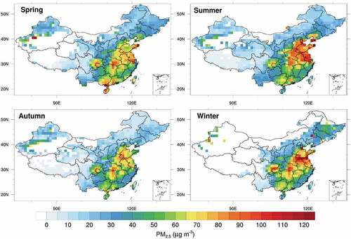
Figure 2 presents the seasonal distribution of satellite-derived PM_2.5 mass concentration over China. Regarding the division of the four seasons, each season consists of three consecutive months. The spring starts with March and ends with May. The winter average has one less observation than other seasons because MODIS products started in March 2000. From the spatial distribution of PM_2.5, there are 6 pollution centers in China, including the area among Hebei-Shandong-Henan provinces (HSH), the Yangtze River Delta (YRD), the Pearl River Delta (PRD), the Jianghan Plain (JHP), the Sichuan Basin (SCB), and the Xinjiang Tarim Basin (XTB). The inversion of aerosol properties using the MODIS DT method is difficult due to the bright surface of desert in XTB, but the concentration changes can be inferred from that in the edge area. Comparing the PM_2.5 among the four seasons, the maximum value mostly appears in winter, with that of 123 μg m⁻³, and the polluted regions are mainly distributed at the HSH, the SCB and the JHP. There are slight polluted regions in the YRD and the PRD, and PM_2.5 in the Northeast (Jilin and Heilongjiang provinces) is also higher in winter than in other seasons. The mean PM_2.5 in winter over China is also the highest among the four seasons, with that of 42 μg m⁻³. However, this may be related to the lack of observations due to the impact of the bright surface in winter. Although the peak of PM_2.5 mass concentration in winter is high, it seems that the spatial distribution of high concentration is restricted in relatively small areas, presumably vicinities of pollution sources owing to unfavorable diffusion conditions. In summer, one can observe that the peak of PM_2.5 mass concentration (107 μg m⁻³) is lower than that in winter but the pollution spreads to larger areas than it does in winter. The PM_2.5 mass concentration averaged in the region of eastern China (110°-120°E, 30°-40°N) in summer (66 μg m⁻³) shows a higher value than that in winter (57 μg m⁻³). The polluted region of PM_2.5 obviously moves from HSH to YRD, and that in Jilin and Heilongjiang provinces move to the coastal areas of Liaoning province in summer. This is related to the high temperature and ambient humidity in the south and coastal areas in summer leading to the easy formation of secondary pollutants. PM_2.5 in the other two polluted regions (JHP and SCB) have reduced to less than 90 μg m⁻³. In the spring, the good diffusion conditions in the northern region cause that the PM_2.5 mass concentration decreases significantly, while that in the PRD and XTB increases. The mean PM_2.5 mass concentration in the region of eastern China is 53 μg m⁻³, higher than that in autumn, because of more dust events in spring. Pollution is significantly weakened in autumn. The polluted regions are mainly concentrated at HSH, JHP and SCB, and PM_2.5 mass concentrations drop overall China, with the highest value of only 90 μg m⁻³.

Figure 2. Seasonal distribution of satellite-derived PM_2.5 mass concentration over China averaged from March 2000 to November 2015.

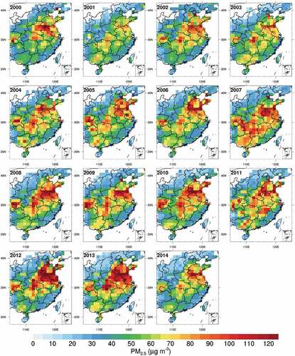
Figure 3 shows the PM_2.5 mass concentration in the winter from 2001 to 2015 in central and eastern China. The PM_2.5 mass concentration increases from 2001 to 2013, though there is a slight decrease in 2002 and 2004. Then, the pollution level drops significantly after 2015, probably influenced by pollution control policies. Except for 2002, the high values of PM_2.5 mass concentration in winters of other years all exceed 100 μg m⁻³, especially in 2013 when it reaches 250 μg m⁻³. From the perspective of the spatial distribution, PM_2.5 mass concentrations in HSH, JHP, and SCB regions have increased year by year, gradually spreading from these pollution centers to the surrounding area, and finally form a large-scale regional pollution in the central and eastern China. After 2015, the PM_2.5 mass concentration decreases and the high-value areas also narrow down significantly. The average value over the central and eastern China drops from 55 μg m⁻³ in 2013 to the lowest value of 43 μg m⁻³ in the 15 years, as same as that in 2002. However, it should be noted that the pollution centers have not disappeared in 2015, and the PM_2.5 mass concentration in the HSH region is still significantly higher than 2002.

Figure 3. The mean value of PM_2.5 mass concentration changes in winter over the central and eastern regions of China (as seen in the figure above) from 2001 to 2015.

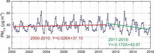
Figure 4 shows the trend of monthly average PM_2.5 over China from March 2000 to December 2015. We find that from 2000 to 2010, PM_2.5 over China shows a slow upward trend, and the interannual increasing rate of PM_2.5 mass concentration is 0.026 μg m⁻³. In June 2003, PM_2.5 has a significantly high value in eastern China, exceeding 60.0 μg m⁻³. This high value of PM_2.5 is related to straw burning and unfavorable weather conditions for diffusion in eastern China (Cao, Zhang, Zheng, & Wang, 2006). From 2011 to 2015, under the policies of air pollution control, the interannual decreasing rate of PM_2.5 mass concentration is 0.172 μg m⁻³ yr⁻¹. PM_2.5 exceeds 60 μg m⁻³ only once in January 2013.

Figure 4. Monthly trend of satellite-derived PM_2.5 over China from March 2000 to December 2015. The red line shows the trend of PM_2.5 from 2000 to 2010, and the green line shows that from 2011 to 2015.

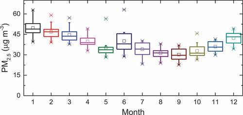
Figure 5 shows the monthly changes of multi-year averaged PM_2.5 in China as a box and whisker plot. The small squares represent the mean values, and the median values of PM_2.5 are indicated by a short line inside each box. The top and bottom edges of each box represent the top and bottom quartiles, and the corresponding whiskers are the outliers. We find that PM_2.5 mass concentration basically runs high in winter, runs low in summer and autumn, and only slightly increases in June and July, which may be related to the burning of straw (May and June) and pollutions caused by photochemical reactions in summer. Also, some errors of PM_2.5 in June and July may be introduced by fewer available observations under the influence of cloud and rain. The highest PM_2.5 mass concentration presents in January during the whole year, with an average value of 50 μg m⁻³. The minimum of the monthly averaged PM_2.5 appears in September, but its upper quartile still exceeds that of August, indicating that some pollution events with high concentrations of PM_2.5 may still occur. This monthly changes of satellite-derived PM_2.5 in Figure 5 agree with the in-situ monitoring.

Figure 5. The monthly changes of multi-year averaged PM_2.5 in China. For the box-and-whisker plot, the mean value is indicated by a square (□), and the median value is indicated by a short line inside the box (-). The top and bottom edges of each box represent the top and bottom quartiles, and the corresponding whiskers are the outliers.

4. Validation with ground-based observations

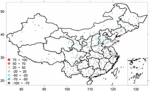
The estimated PM_2.5 mass concentrations are evaluated by comparison with ground-based PM_2.5 data. Ground-based PM_2.5 from two sources are used. One comes from 1442 ground sites in 372 cities over China during 2013–2015, published by the China National Environmental Monitoring Centre. The ground observed PM_2.5 from sites are averaged at city scale in order to enhance the spatial representation of ground stations. The other part is obtained from additional sources to extend the validation to the period before 2013, i.e. from the U.S. embassies in Beijing (2008–2015), Shanghai (2011–2015), Guangzhou (2011–2015), Chengdu (2012–2015) and the Hongkong environmental protection agency (2000–2015). Figure 6 shows the biases of satellite-derived PM_2.5 in cities over China averaged from 2013–2015. The sites with bias within ±20 μg m⁻³ account for 63.4% of all sites. Only a few sites (7.1%) in Shandong, Jiangsu and Shanghai have a bias larger than 20 μg m⁻³ of PM_2.5. At some northern regions, the sites where PM_2.5 are underestimated (bias < −20 μg m⁻³) account for 29.4%.

Figure 6. The biases of satellite-derived PM_2.5 averaged from 2013–2015 over China in 372 cities.

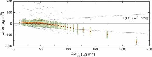
Figure 7 shows the errors of the satellite-derived monthly PM_2.5, which are derived from 7116 data pairs (satellite-derived v.s. in-situ) and divided into 72 bins. We then calculate the median, mean, standard deviation and maximum and minimum of errors in every bin. The expected error (dashed line in Figure 7) is defined as the envelope encompassing the standard deviation of error, which is about ±(15 μg m⁻³ + 30%) as compared with in situ observations. We find that with the increase of in-situ observed PM_2.5 concentration, the error of satellite-derived PM_2.5 increases. The median error is underestimated by more than 10 μg m⁻³ at about 70 μg m⁻³ of in-situ concentration. The error shows a slight overestimation at less than 50 μg m⁻³ and an underestimation at more than 65 μg m⁻³. The mean error in this interval (50–65 μg m⁻³) tends to be 0.0 (0.076 μg m⁻³). The standard deviations of errors are basically within the lower limit of the expected error when in-situ PM_2.5 is less than 85 μg m⁻³, whereas they often exceed the upper limit. From the extreme values of PM_2.5, the high value runs the risk of being underestimated, while the low value is more likely to be overestimated, which is also related to the inversion bias trend of AOD. The frequency (73.2%) within the expected error and historical trend comparison can be found in Zhang et al. (2020).

Figure 7. Comparison of the satellite-derived monthly PM_2.5 with in situ measurements. The expected error envelope is ±(15 μg m⁻³ + 30%). We set 72 bins in PM_2.5 levels to calculate the median error (+), mean error (□), standard deviation (bar) and maximum and minimum errors (-).

5. Data set value

Compared with atmospheric particulate matter in coarse mode, PM_2.5 with relatively small particle size contains an amount of toxic substances, and has a long residence time and transportation distance in the atmosphere. Therefore, it is harmful to human health and air quality, and it has great impacts on climate changes as well. In China, the pollution of atmospheric fine particles is a challenging environmental issue. The systematic near-surface PM_2.5 monitoring has not been fully implemented in China until 2013, thus the lack of historical data is a key obstacle to historical analysis of PM_2.5 long-term trends.

This paper provides a historical data set of PM_2.5 mass concentration with a spatial resolution of 1°×1° over land of China from 2000 to 2015. The PM_2.5 mass concentration is estimated based on the PMRS remote sensing model, including size cutting, volume visualization, bottom isolation and particle drying procedures. The input data of PMRS model are satellite remote sensing (AOD & FMF) and NCAR FNL meteorological reanalysis data (PBLH & RH), which are completely independent of ground observations of PM_2.5. Therefore, our data set can be objectively validated by ground observations to ensure the accuracy.

In addition, the PMRS model conforms to the laws of physics, which ensures the global consistency of PM_2.5 concentration estimation. In other words, compared with statistical methods, the accuracy of our data set does not change with the distribution of ground sites; and compared with model methods, our data set is not affected by the uncertainty of model emission sources and the completeness of chemical reaction mechanism, which increases the robustness of the data set. The historical PM_2.5 data set can not only provide basic data for the studies of human exposure to particulate matter, but also serve for historical assessment of air quality.

Open scholarship

This article has earned the Center for Open Science badge for Open Data. The data are openly accessible at http://www.dx.doi.org/10.11922/sciencedb.j00076.00061.

Disclosure statement

No potential conflict of interest was reported by the author(s).

Data availability statement

The data that support the findings of this study are openly available in SONET at https://www.sonet.ac.cn/ and in Science Data Bank at http://www.dx.doi.org/10.11922/sciencedb.j00076.00061.

Additional information

Funding

The research presented in this paper was funded by the National Key R&D Program of China (Grant Number 2016YFE0201400), the Hainan Provincial Natural Science Foundation of China (Grant Number 418QN302), the National Natural Science Foundation of China (Grant Numbers 41925019, 41671367) and the National Key B&R Program of China [2016YFE0201400].

Notes on contributors

Ying Zhang

Ying Zhang received her Ph.D. degree in cartography and geographical information system from University of Chinese Academy of Sciences, Beijing, China, in 2013, and her bachelors degree from Nanjing University of Information Science and Technology, China, in 2006. She is currently an Associate Professor at Aerospace Information Research Institute, Chinese Academy of Sciences, China. She has co-authored over 50 peer-reviewed journal publications. Her research interests include aerosol remote sensing and modeling.

Zhengqiang Li

Zhengqiang Li received his Ph.D. degree in optics from Anhui Institute of Optics and Fine Mechanics, Chinese Academy of Sciences, Hefei, China, in 2004. Professor Zhengqiang Li is the Executive Director of National Engineering Laboratory for Remote Sensing Satellite Applications in Aerospace Information Research Institute, Chinese Academy of Sciences, China. He serves as the Vice Director of State Environmental Protection Key Laboratory of Satellite Remote Sensing. He is also the PI of the Chinese sun‒sky radiometer observation network (SONET). He has co-authored over 190 peer-reviewed journal publications. His research interests include aerosol and atmospheric environment.

Yuanyuan Wei

Yuanyuan Wei received her Ph.D. degree in Aerospace Information Research Institute, Chinese Academy of Sciences, Beijing, China, in 2020. She received her bachelors degree from Nanjing University of Information Science and Technology. She is currently a Post-doc in National Engineering Laboratory for Remote Sensing Satellite Applications, Aerospace Information Research Institute, Chinese Academy of Sciences. Her research interests include aerosol remote sensing and atmospheric environment.

Zongren Peng

Zongren Peng received his Ph.D. degree in Theoretical Physics from Pierre and Marie Curie University - Paris 6 and Institute of Theoretical Physics in French Alternative Energies and Atomic Energy Commission in 2012. He is currently a research assistant at Aerospace Information Research Institute, Chinese Academy of Sciences, China. His research interests focus on remote sensing retrieval, particle physics and statistics.

References

- Brokamp, C., Jandarov, R., Hossain, M., & Ryan, P. (2018). Predicting daily urban fine particulate matter concentrations using a random forest model. Environmental Science & Technology, 52(7), 4173–4179.
- Cao, G., Zhang, X., Zheng, F., & Wang, Y. (2006). Estimating the quantity of crop residues burnt in open field in China. Resources Science, 28(1), 9–13.
- Chu, D. A., Kaufman, Y. J., Zibordi, G., Chern, J. D., Mao, J., Li, C. C., & Holben, B. N. (2003). Global monitoring of air pollution over land from the earth observing system-terra moderate resolution imaging spectroradiometer (MODIS). Journal of Geophysical Research: Atmospheres, 108(D21). doi:10.1029/2002jd003179
- de Leeuw, G., Sogacheva, L., Rodriguez, E., Kourtidis, K.,Georgoulias, A. K., Alexandri, G., Amiridis, V., Proestakis, E.,Marinou, E., Xue, Y., and van der A, R. (2018). Two decades ofsatellite observations of AOD over mainland China using ATSR-2, AATSR and MODIS/Terra: data set evaluation and large-scalepatterns. Atmospheric Chemistry & Physics, 18,1573–1592
- Engel-Cox, J. A., Hoff, R. M., Rogers, R., Dimmick, F., Rush, A. C., Szykman, J. J., … Zell, E. R. (2006). Integrating lidar and satellite optical depth with ambient monitoring for 3-dimensional particulate characterization. Atmospheric Environment, 40(40), 8056–8067.
- Engel-Cox, J. A., Holloman, C. H., Coutant, B. W., & Hoff, R. M. (2004). Qualitative and quantitative evaluation of MODIS satellite sensor data for regional and urban scale air quality. Atmospheric Environment, 38(16), 2495–2509.
- Fang, X., Zou, B., Liu, X., Sternberg, T., & Zhai, L. (2016). Satellite-based ground PM2.5 estimation using timely structure adaptive modeling. Remote Sensing of Environment, 186, 152–163.
- Gupta, P., Christopher, S. A., Wang, J., Gehrig, R., Lee, Y., & Kumar, N. (2006). Satellite remote sensing of particulate matter and air quality assessment over global cities. Atmospheric Environment, 40(30), 5880–5892.
- He, Q., & Huang, B. (2018). Satellite-based mapping of daily high-resolution ground PM2.5 in China via space-time regression modeling. Remote Sensing of Environment, 206, 72–83.
- Hu, X., Belle, J. H., Meng, X., Wildani, A., Waller, L. A., Strickland, M., & Liu, Y. (2017). Estimating PM2.5 concentrations in the conterminous United States using the random forest approach. Environmental Science & Technology, 51(12), 6936–6944.
- Koelemeijer, R. B. A., Homan, C. D., & Matthijsen, J. (2006). Comparison of spatial and temporal variations of aerosol optical thickness and particulate matter over Europe. Atmospheric Environment, 40(27), 5304–5315.
- Kokhanovsky, A. A., Prikhach, A. S., Katsev, I. L., & Zege, E. P. (2009). Determination of particulate matter vertical columns using satellite observations. Atmospheric Measurement Techniques, 2(2), 327–335.
- Levy, R. C., Remer, L. A., Kleidman, R. G., Mattoo, S., Ichoku, C., Kahn, R., & Eck, T. F. (2010). Global evaluation of the Collection 5 MODIS dark-target aerosol products over land. Atmospheric Chemistry & Physics, 10(21), 10399–10420.
- Li, Y., Lin, C. Q., Lau, A. K. H., Liao, C. H., Zhang, Y. B., Zeng, W. T., … Tse, T. K. T. (2015). Assessing long-term trend of particulate matter pollution in the pearl river delta region using satellite remote sensing. Environmental Science & Technology, 49(19), 11670–11678.
- Li, Z., Zhang, Y., Shao, J., Li, B., Hong, J., Liu, D., … Qie, L. (2016). Remote sensing of atmospheric particulate mass of dry PM2.5 near the ground: Method validation using ground-based measurements. Remote Sensing of Environment, 173, 59–68.
- Lin, C. Q., Li, Y., Yuan, Z. B., Lau, A. K. H., Li, C. C., & Fung, J. C. H. (2015). Using satellite remote sensing data to estimate the high-resolution distribution of ground-level PM2.5. Remote Sensing of Environment, 156, 117–128.
- Liu, Y., Paciorek, C. J., & Koutrakis, P. (2009). Estimating Regional Spatial and Temporal Variability of PM2.5 Concentrations Using Satellite Data, Meteorology, and Land Use Information. Environmental Health Perspectives, 117(6), 886–892.
- Ma, Z., Hu, X., Huang, L., Bi, J., & Liu, Y. (2014). Estimating ground-level PM2.5 in China using satellite remote sensing. Environmental Science & Technology, 48(13), 7436–7444.
- Ma, Z., Hu, X., Sayer, A. M., Levy, R., Zhang, Q., Xue, Y., … Liu, Y. (2016). Satellite-based spatiotemporal trends in PM2.5 concentrations: China, 2004–2013. Environmental Health Perspectives, 124(2), 184–192.
- Petters, M. D., & Kreidenweis, S. M. (2007). A single parameter representation of hygroscopic growth and cloud condensation nucleus activity. Atmospheric Chemistry & Physics, 7(8), 1961–1971.
- Raut, J. C., & Chazette, P. (2009). Assessment of vertically-resolved PM10 from mobile lidar observations. Atmospheric Chemistry & Physics, 124(2), 8617–8638.
- Raut, J. C., Chazette, R., & Fortain, A. (2009). New approach using lidar measurements to characterize spatiotemporal aerosol mass distribution in an underground railway station in Paris. Atmospheric Environment, 43(3), 575–583.
- Shen, H., Li, T., Yuan, Q., & Zhang, L. (2018). Estimating regional ground-level PM2.5 directly from satellite top-of-atmosphere reflectance using deep belief networks. Journal of Geophysical Research: Atmospheres, 123(24), 13, 875–13,886.
- Van Donkelaar, A., Martin, R. V., Brauer, M., & Boys, B. L. (2015). Use of satellite observations for long-term exposure assessment of global concentrations of fine particulate matter. Environmental Health Perspectives, 123(2), 135–143.
- Van Donkelaar, A., Martin, R. V., Brauer, M., Kahn, R., Levy, R., Verduzco, C., & Villeneuve, P. J. (2010). Global estimates of ambient fine particulate matter concentrations from satellite-based aerosol optical depth: Development and application. Environmental Health Perspectives, 118(6), 847–855.
- Van Donkelaar, A., Martin, R. V., Li, C., & Burnett, R. T. (2019). Regional estimates of chemical composition of fine particulate matter using a combined geoscience-statistical method with information from satellites, models, and monitors. Environmental Science & Technology, 53(5), 2595–2611.
- Van Donkelaar, A., Martin, R. V., & Park, R. J. (2006). Estimating ground-level PM 2.5 using aerosol optical depth determined from satellite remote sensing. Journal of Geophysical Research: Atmospheres, 111(D21), D21.
- van Donkelaar A., Martin R.V., Pasch A.N., Szykman J.J., ZhangL., Wang Y.X., and Chen D. (2012). Improving the accuracy of dailysatellite-derived ground-level fine aerosol concentration estimatesfor North America. Environmental Science & Technology, 46,11971–11978.
- Wang, J., & Christopher, S. A. (2003). Intercomparison between satellite-derived aerosol optical thickness and PM2.5 mass: Implications for air quality studies. Geophysical Research Letters, 30(21). doi:10.1029/2003gl018174
- Wang, J., Xu, X. G., Spurr, R., Wang, Y. X., & Drury, E. (2010b). Improved algorithm for MODIS satellite retrievals of aerosol optical thickness over land in dusty atmosphere: Implications for air quality monitoring in China. Remote Sensing of Environment, 114(11), 2575–2583.
- Wei, J., Peng, Y., Peng, Y., Sun, L., Peng, Y., Sun, L., & Cribb, M. (2019). Estimating 1-km-resolution PM2.5 concentrations across China using the space-time random forest approach. Remote Sensing of Environment, 231, 111221.
- Wei Y., Li Z., Zhang Y., Chen C., Xie Y., Lv Y. and Dubovik O.(2021). Derivation of PM10 mass concentration from advancedsatellite retrieval products based on a semi-empirical physicalapproach. Remote Sensing of Environment, 256, 112319.
- Zhang, Y., Li, Z., Chang, W., Zhang, Y., De Leeuw, G., & Schauer, J. J. (2020). Satellite observations of PM2.5 changes and driving factors based forecasting over China 2000–2025. Remote Sensing, 12(16), 2518.
- Zhang, Y., & Li, Z. Q. (2015). Remote sensing of atmospheric fine particulate matter (PM2.5) mass concentration near the ground from satellite observation. Remote Sensing of Environment, 160, 252–262.