Living Earth: Implementing national standardised land cover classification systems for Earth Observation in support of sustainable development

ABSTRACT

Earth Observation (EO) has been recognised as a key data source for supporting the United Nations Sustainable Development Goals (SDGs). Advances in data availability and analytical capabilities have provided a wide range of users access to global coverage analysis-ready data (ARD). However, ARD does not provide the information required by national agencies tasked with coordinating the implementation of SDGs. Reliable, standardised, scalable mapping of land cover and its change over time and space facilitates informed decision making, providing cohesive methods for target setting and reporting of SDGs. The aim of this study was to implement a global framework for classifying land cover. The Food and Agriculture Organisation’s Land Cover Classification System (FAO LCCS) provides a global land cover taxonomy suitable to comprehensively support SDG target setting and reporting. We present a fully implemented FAO LCCS optimised for EO data; Living Earth, an open-source software package that can be readily applied using existing national EO infrastructure and satellite data. We resolve several semantic challenges of LCCS for consistent EO implementation, including modifications to environmental descriptors, inter-dependency within the modular-hierarchical framework, and increased flexibility associated with limited data availability. To ensure easy adoption of Living Earth for SDG reporting, we identified key environmental descriptors to provide resource allocation recommendations for generating routinely retrieved input parameters. Living Earth provides an optimal platform for global adoption of EO4SDGs ensuring a transparent methodology that allows monitoring to be standardised for all countries.

KEYWORDS:

• Land cover
• FAO LCCS
• open data cube
• sustainable development goals
• environmental descriptors

1. Introduction

The United Nations 2030 Agenda for Sustainable Development represents a global agenda for participating nations to strive for economic, social and environmental sustainability by 2030 (DESA, 2016). The Sustainable Development Goals (SDGs) were developed to identify and monitor unsustainable practices, providing the opportunity for nations to intervene where necessary to improve sustainable development. The SDGs include 17 thematic goals and 169 standardised targets to strive for sustainable development among all nations, with 231 indicators to monitor performance towards agreed targets (UNGA, 2015). However, most targets designated for achievement by 2020 were not met, and reported indicators from participating nations suggest that many will still be some way from attainment by 2030 (Kavvada et al., 2020). A fundamental limitation in progressing the SDGs has been identified around timely, reliable, standardised and openly available information (UNGA, 2019). Nations have expressed concern that without key data to support target setting and tracking of progress, through explicit information of the performance of an indicator over time, no reasonable policy and management changes can be actioned to change current trajectories towards attainment.

Earth Observation (EO) has been recognised as a key data source for metrics related to the SDGs, providing global data to identify landscape types and composition and their change over time. EO has the capacity to support reporting and tracking of approximately 40 targets and 30 indicators for many SDGs: well-developed examples include Goal 6 (Clean water and sanitation), Goal 11 (Sustainable cities), Goal 14 (Life below water), and Goal 15 (Life on land) (EO4SDGs, 2020; Estoque, 2020; Metternicht, Mueller, & Lucas, 2020; Paganini et al., 2018). Advances in data availability (e.g. Landsat (Woodcock et al., 2008) and Copernicus (Berger et al., 2012) missions), storage and computational capacity (e.g. Amazon Web Services, Google Earth Engine (see Gomes, Queiroz, & Ferreira, 2020)), and analytical capabilities (e.g. Open Data Cube (Killough, 2018), Machine learning (see Ferreira, Iten, & Silva, 2020)) have provided a wide range of users access to global coverage analysis-ready data (ARD). However, ARD does not provide the information required by national agencies tasked with coordinating implementation of SDGs (Kavvada et al., 2020). Instead, they require standardised and informative end user products derived from ARD to track progress towards agreed targets. This includes land cover and its change over time – detailed information that contributes to the mapping and reporting on 14 of the 17 SDGs (EO4SDGS, 2020). However, many nations lack access to an operational, standardised land cover product.

Land cover maps are an essential information component for planning and managing sustainable development, often utilised to establish baseline conditions against which to monitor change across a range of spatial, temporal and thematic scales (Gómez, White, & Wulder, 2016; Rogan & Chen, 2004). Operational monitoring of land cover requires timely, reliable and repeatable mapping over multiple time-steps and at spatial scales relevant to policy and management (Franklin & Wulder, 2002). Robust methods that allow seamless integration of new observations or data and a high degree of confidence for change detection are greatly valued. However, most existing products do not provide the operational requirements for SDG target setting and reporting at a national level, and many are also not comparable between countries (Metternicht et al., 2020). In addition, existing global and continental land cover maps are often produced at spatial scales not suitable for SDG reporting units. These include IGBP DISCover (1 km; Loveland et al., 2000), UMD Land Cover (1 km; Hansen, DeFries, Townshend, & Sohlberg, 2000), GlobCover (300 m; Arino et al., 2008), Corine Land Cover (300 m; Bossard, Feranec, & Otahel, 2000), ESA CCI Land Cover (300 m; Bontemps et al., 2013), and MODIS Land Cover (250 m; Friedl et al., 2010). Challenges associated with high resolution land cover mapping at large scales are diminishing with increased data availability and computational capacity (e.g. Global 30 m, Chen et al., 2014; Europe 10 m, Venter & Sydenham, 2021) and attention is now shifting to harmonise land cover maps (Yang, Li, Chen, Zhang, & Xu, 2017). A component of this is to adopt systems for mapping land cover that are consistent terminologically (e.g. forest vs woodland), semantically (e.g. trees are plants > 2 m height) and cartographically (e.g. map products are comparable). This is becoming of increased importance given enhanced capacity for mapping land cover across large areas and on a repeat basis (e.g. Calderón-Loor, Hadjikakou, & Bryan, 2021; Li, Qiu, Ma, Schmitt, & Zhu, 2020).

To comprehensively support international initiatives for sustainable development, land cover maps must prioritise methods that are transparent (i.e. FAIR principles; Wilkinson et al., 2016) and transferable (e.g. across sensors and platforms, utilising available computational resources), with consistent semantics and taxonomies to facilitate robust and routine generation. The Land Cover Classification System (LCCS), developed by the Food and Agriculture Organisation (FAO; Di Gregorio & Jansen, 2000), provides a taxonomy that is fundamentally well suited to consistent classification of land cover. The FAO LCCS attempts to fix historical issues of semantics with land cover classifications, identifying the need to align landscape descriptions with their “mapability” (Di Gregorio, 2016). LCCS is a semantically-driven integrated system, providing a taxonomy with a high level of descriptive detail that is consistent and comparable at different scales and over time, and applicable to any geographic location globally. As an internationally recognised taxonomy, land cover maps using the LCCS taxonomy are also interoperable with end-user requirements (i.e. classes generated closely align with habitat taxonomies that are widely used by ecologists) (Atyeo & Thackway, 2006; Kosmidou et al., 2014).

Application of the FAO LCCS for use with EO data has been established using the Earth Observation Data for Ecosystem Monitoring (EODESM) system (Lucas & Mitchell, 2017; Lucas et al., 2019, 2020). Unlike other EO implementations of the LCCS, which generally base their classifications on the “end classes” in the LCCS taxonomy, the EODESM system follows the sequence of classifications through the hierarchy using products derived from EO data. Rather than focusing on providing the best classification algorithm, the EODESM system places emphasis on retrieving continuous and categorical environmental descriptors; biophysical input variables with predefined units or categories (see Lucas & Mitchell, 2017; Lucas et al., 2019; Planque et al., 2020). These are then combined subsequently to construct the LCCS classes. The advantage of this classification approach is that it is relevant and applicable to any site globally and can be applied independent of scale and time. EODESM demonstrated the global applicability of the LCCS taxonomic framework with an initial focus on national parks (Lucas & Mitchell, 2017), as well as sites in Australia (Lucas et al., 2019) and Malaysia (Lucas et al., 2020) and most recently for Wales (Planque et al., 2020).

The FAO LCCS system has been fully designed and comprehensively documented (LCCS-2: LCCS software version 2; Di Gregorio, 2005). However, no systematic implementation is available for EO data. EODESM demonstrates the capacity to implement a fully interoperable EO software product for application. Several prior land cover products recognise the flexibility and comprehensive nature of LCCS and have implemented some aspects of the LCCS-2 on a fit-for-purpose basis (e.g. GlobCover, Bicheron et al., 2008; Dynamic Land Cover Dataset, Lymburner, Tan, Mueller, Thackway, & Thankappan, 2011; North American Land Change Monitoring System, Latifovic et al., 2012). Notably, several semantic issues are not fully resolved with LCCS-2 that have remained a challenge for EO implementation, often requiring users to modify taxonomic classes to suit requirements or only adopt LCCS-2 taxonomies and not the hierarchical-modular structure. Resolving semantic challenges with LCCS-2 for EO application would encourage widespread adoption and reduce barriers to using the LCCS-2 system in its entirety.

The aim of this study was to implement a global framework for classifying land cover in support of consistent and comparable reporting on the SDGs. The FAO LCCS provides a global land cover taxonomy suitable to comprehensively support SDG target setting and reporting. We present a fully implemented FAO LCCS-2 optimised for EO data; Living Earth, an open-source software package that can be readily applied using existing national EO infrastructure and satellite data. To ensure easy adoption of Living Earth for SDG reporting, we identified key environmental descriptors of FAO LCCS-2 to provide recommendations on resource allocation for generating routinely retrieved input parameters. In addition, we examined two national implementations using different EO infrastructure and satellite data, Australia and Wales (UK), providing recommendations on resource allocation for further development.

2. Methods

2.1. FAO LCCS-2 and EODESM

The FAO LCCS-2 framework is hierarchical, consisting of a dichotomous and a modular-hierarchical phase. The dichotomous phase is a binary decision tree providing eight (8) output classes that determine broad landscape types (Figure 1). At level 1 (L1), areas that are primarily vegetated are differentiated from those that are primarily non-vegetated. Terrestrial and aquatic areas are subsequently differentiated at level 2 (L2). Primarily vegetated areas are further classified based on human activities, generating four primarily vegetated level 3 (L3) classes including a) cultivated and managed terrestrial areas, b) natural and semi-natural vegetation, c) cultivated aquatic or regularly flooded areas, and d) natural and semi-natural aquatic or regularly flooded vegetation. Similarly, primarily non-vegetated areas are separated into a) artificial surfaces and associated expanses, b) naturally bare areas, c) natural water bodies, and d) artificial water bodies.

Figure 1. The Living Earth LCCS-2 implementation. The hierarchy for the dichotomous phase (L1 – L3) visualised vertically and the modular-hierarchical phase (L4) visualised horizontally. Each level 3 broad land cover type has associated level 4 additional descriptors that are also hierarchical (i.e. between 2–5 tiers). T; tier L; level. Asterisk (*) indicates land cover classes not required for subsequent environmental descriptors in the hierarchy

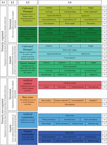
The subsequent modular-hierarchical phase (referred hereon in as level 4; L4) provides increasingly detailed landscape descriptions tailored to each of the broad land cover types across the eight level 3 classes (Figure 1). In this phase, the generation of the land cover class is given by combining a set of predefined land cover classifiers that also operate in a hierarchy as level 4 “tiers”. The classification system generates mutually exclusive land cover classes, which comprise a unique boolean formula (a coded string of classifiers used) and a structured description of the land cover class based on level 4 tiers. At any position in the hierarchy the user can stop, and a mutually exclusive class is generated. The system created is a highly flexible a priori land cover classification in which each category is clearly and systematically defined to provide internal consistency.

2.2. Living Earth: LCCS-2 optimised for EO

The design of Living Earth closely followed the LCCS-2 documentation (Di Gregorio, 2005) to maintain the fundamental principles and qualities of LCCS semantics and its taxonomic framework. This included maintaining the LCCS structure, dichotomous and modular-hierarchical phases, and broad land cover types with additional descriptors. Several modifications were made from LCCS-2 environmental descriptors for the implementation of Living Earth, with these focused on optimising LCCS-2 for readily available EO data. To ensure easy adoption for end users, we considered a practical data driven approach to implementing LCCS-2, in particular the flexibility and “mapability” of the system (Di Gregorio, 2016). The intent of any additional environmental descriptors was examined carefully to ensure they enhance the overall description of the land cover class. All modifications and assumptions undertaken are described below.

2.2.1. Key modifications and assumptions

The FAO LCCS level 4 as a hierarchical design is composed of tiers, whereby preceding land cover descriptors must have input data before additional environmental descriptors can be added (Figure 1). These tiers are also interdependent, where a landscape class (i.e. lifeform) is required before additional information within the same tier can be added to the landscape description (i.e. cover). Living Earth maintains the hierarchy of level 4 descriptions, however does not require interdependency within tiers. Specifically, the generation of routinely derived descriptors for some classes are already achievable from EO data and provide valuable landscape information (e.g. vegetation cover and height). Importantly, further landscape descriptions for a proceeding tier still require all classes of the preceding tier to be valid. For example, classes at tier 1 of level 4 for terrestrial vegetated areas, that is lifeform, cover and height, are not dependent on each other for a valid landscape description. However, all are required to progress to tier 2 descriptors. Inherent dependencies within these classes are still relevant, for example, the class “trees” in the category “lifeform” cannot be assigned to the class “height < 2 m”.

The FAO LCCS definition of vegetation strata is an ecological definition manifest through relationships of vegetation lifeform, cover and height. This can be difficult to determine from EO and particularly dependent on the approaches to generate lifeform, cover and height metrics. Defining strata consistently is critical, as this impacts the assignment of land covers to several strata classes (e.g. lifeform, cover and height of second strata as well as crop combinations and crop lifeforms). To optimise for the use of EO to generate consistent and comparable landscape descriptors for a variety of landscapes, we only use height to differentiate the second strata. For example, if the first strata are lifeform of trees 2–5 m in height, the second strata must be less than 2–5 m in height and is therefore not a sub strata of tree vegetation.

Living Earth landscape descriptions do not assume all data are available and therefore can provide landscape classifications with partial LCCS-2 level 4 descriptions. The FAO LCCS has approximately 12,000 unique complete landscape descriptions, assuming all required input data are available. Due to the inherent limitations of EO data, as well as ongoing research to retrieve or classify environmental descriptors, it is impractical to expect all data requirements for a complete level 4 landscape description. Living Earth therefore provides an accessible data-driven approach to describe environmental landscapes, where valid and useful landscape descriptors can be produced with available data. This allows greater flexibility to the LCCS framework and encourages greater uptake for land cover classification.

2.2.2. Technical modifications

To align the software design and implementation with the LCCS-2 in the most effective yet simplistic way possible, while ensuring LCCS remains intuitive, several technical modifications were employed. These are detailed briefly here and extensively documented in the software code.

Alphanumeric codes align to terrestrial (semi) natural vegetation

LCCS descriptors are a concatenation of alphanumeric codes that detail each level 4 category contributing to the description (e.g. A12.A1.A10.B5.C1). Alphanumeric codes in LCCS-2 of a level 4 category may not be identical for each level 3 broad land cover type (e.g. tree lifeform is A1 for Cultivated and managed, yet is A3 for (semi) natural). These vary for each level 3 class, where a level 4 class attributes descriptors to multiple level 3 classes (i.e. lifeform, cover, height). All level 4 codes in Living Earth are aligned to terrestrial (semi) natural vegetation. This provides consistency within level 4 classes and efficiency for input layers and concatenation in level 4 classification. In addition, several level 4 categories were merged to simplify the classification (i.e. one lifeform layer input is used for classifying lifeform of all vegetated level 3 classes) as well as broad categories removed in favour of specificity (e.g. cover classes closed to open 15–100% and 40–100% are not useful ecological categories to determine from EO). All are documented in the software code for each level 4 class to show deviation from FAO LCCS-2.

Class categorical boundaries altered to non-overlapping ranges

FAO LCCS-2 utilises overlapping class boundaries for several continuous inputs (e.g. cover: closed > 60–70%). This represents the ambiguity associated with quantitative measurement and meaningful ecological disaggregation of environmental descriptors. Living Earth is optimised for EO, requiring distinct class boundaries for meaningful implementation of mapping. Class categorical boundaries were altered to give non-overlapping ranges, centred on the middle of the FAO LCCS-2 range (i.e. LCCS-2, > 60–70%: Living Earth, > 65%). This modification was introduced for all relevant classes including cover, height, and second strata cover and height.

Additional environmental descriptors and attribution

LCCS-2 level 4 classes were reviewed to optimise for EO inputs. A new class for tidal areas was generated, separating these from the water persistence categories because a) tidal areas can be perennial/non-perennial and thus may conflict with water persistence categories and b) EO-derived products available to identify tidal areas are increasingly being generated on a routine basis (e.g. Bishop-Taylor, Sagar, Lymburner, & Beaman, 2019; Sagar, Roberts, Bala, & Lymburner, 2017).

Living Earth includes height and cover attributes for cultivated and managed areas. These are not included in LCCS-2; however, they were deemed useful environmental descriptors that could be retrieved from EO. Moreover, several agricultural descriptors can be difficult to derive from EO data and including height and cover helps to provide some description of the cultivated landscape with a reasonable degree of accuracy.

2.3. Software design

Living Earth was designed as an open-source Python library, built on top of xarray (Hoyer & Hamman, 2017) and NumPy (Harris et al., 2020), and utilising other established Python libraries for data import and export, such as GDAL (GDAL/OCR Contributors, 2021), Rasterio (Gillies, 2019) and Open Data Cube (Killough, 2018; Killough, Siqueira, & Dyke, 2020). We followed high standards of software design, including version control and unit testing for LCCS classification outputs. The software design was based on applicability for easy adoption and understanding for a broad range of end users, as well as LCCS structure and modifications based on EO implementation (Figure 2).

Figure 2. Software design schematic showing ingestion of the data and application of rules to produce level 3 and level 4 classification outputs as both data (8-bit/n-band raster) and coloured RGB images for visualisation

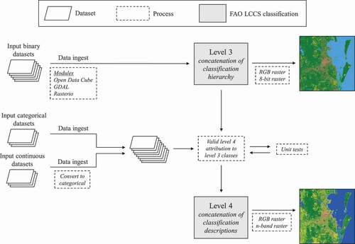
Living Earth provides high data input flexibility, with modules interfacing with GDAL (via rasterio), Open Data Cube (ODC) and RIOS (for object-based classification using raster attribute tables; Gillingham & Flood, 2014). Initially, 5 binary input datasets are required for the level 3 classification. These include a vegetated/non-vegetated layer, water/non-water layer, cultivated/natural vegetation layer, artificial surface/bare areas layer, and artificial water/natural water layer. The level 3 classification is then simply a concatenation of the 5 input layers in the hierarch to derive 8 broad landscape types. An 8-bit raster, coded with LCCS-2 level 3 values (i.e. 111, 112, 123, 124, 215, 216, 227, 228) and three band image (RGB), coloured by class for visualisation, are provided as an initial output.

Level 4 input layers can be categorical or continuous (i.e. cover, height, urban density), where continuous are converted to categorical definitions as specified by LCCS-2 (unless altered as stated in section 2.2). Each level 4 layer is then applied to the relevant level 3 category where any dependencies on other level 4 layers are met. Valid level 4 landscape descriptions are confirmed via unit testing. Level 4 classification is then a concatenation of the level 4 layers, with this providing unique alphanumeric landscape descriptions. An n-band raster, representing each level 4 class input as a single band and RGB image, with each class coloured based on the Living Earth LCCS Level 4 colour scheme, are provided as a final output.

2.4. Key environmental descriptors

Key environmental descriptors were identified for Living Earth using variable importance scores. Variable importance was defined as the reoccurrence of an input layer to produce all outputs for each broad landscape type, calculated by summing the total times categories from an input class were used divided by the total number of unique outputs. A relative variable importance score was calculated for each input variable for each broad landscape. As a consequence of the large number of input combinations, a python workflow was developed that ran the Living Earth system by randomly selecting from all possible input variables for each broad landscape types provided from level 3. These were then used to generate unique output class identifier codes with the associated description. For each level 3 class, 10,000 random selections (samples) were undertaken per run and the classification was run 1000 times, with this generating up to 10 million LCCS-2 land cover class combinations. When no new output classes were found, the workflow terminated.

3. Results

3.1. Software design

Living Earth provides a fully implemented FAO LCCS-2 optimised for EO. Current data ingest classes allow the classification to be applied to any rasterised spatial data (e.g. Landsat, Sentinel-1/2, Lidar derived surfaces, airborne imagery, drone imagery), with the capacity to apply the classification scheme to non-raster data (e.g. tables, databases). The plugin architecture of landscape descriptors at level 4 allows for the addition of environmental descriptors pertinent to each use case. Moreover, landscape classifications can occur with limited data input, and all inputs do not need to be present to generate a valid unique landscape description. Living Earth has been optimised for high-performance computing, with tested compatibility on several national super-computing facilitates (e.g. Australia’s National Computational Infrastructure (NCI), Supercomputing Wales) and cloud services (e.g. Amazon Web Services (AWS)). This is particularly useful for national implementations of LCCS that require a routine and flexible workflow. Living Earth is an open-source software package under Apache 2.0 license, available on bitbucket (https://bitbucket.org/au-eoed/livingearth_lccs).

3.2. Living Earth: LCCS-2 optimised for EO

FAO LCCS provides approximately 12,000 unique landscape descriptions through combinations of level 4 inputs. Living Earth provides approximately 573,307 unique landscape descriptions utilising the same fundamental framework. The pronounced increase in unique descriptions is attributed to the key modifications to optimise for EO implementation (section 2.2). Unique landscape descriptions specific to vegetation accounted for > 99% of all unique descriptors, with non-vegetative classes providing only 720 unique landscape descriptions (Table 1). All unique landscape descriptors are provided in the supplementary material.

Table 1. Living Earth unique landscape descriptor codes and example descriptions for each level 3 landscape type

Level 3 landscape type	Unique landscape descriptors	Alphanumeric example	Landscape description example
Terrestrial Cultivated/Managed	466699	A11.A1.A10.B10.D1.E1.B8.B1.C1.D6.D8 A11.A5.A16.B11.D4.E6.B6.B4.C2.D1	Cultivated Terrestrial Vegetated: Woody Closed (> 65%) (< 0.5 m) Broad-leaved Evergreen Medium to large (> 2 ha) field(s) Single crop Irrigated Drip Fallow system Cultivated Terrestrial Vegetated: Forbs Scattered (1 to 4%) (0.8 to 3 m) Scattered (clustered) Medium (2–5 ha) field(s) Multiple crop Cultural Practice (Rainfed)
Terrestrial (Semi) Natural	21979	A12.A1.A10.B5.D1.E2.C2.F2.F10 A12.A4.A13.B9.D2.E3.C1.F2.F6.F10	Natural Terrestrial Vegetated: Woody Closed (> 65%) (> 14 m) Broad-leaved Deciduous Fragmented Second layer present Sparse (1 to 15%) Natural Terrestrial Vegetated: Shrubs Open (15 to 40%) (0.5 to 2 m) Needle-leaved Mixed Continuous Second layer present Herbaceous Sparse (1 to 15%)
Aquatic Cultivated/Managed	7970	A23.A1.A10.B10.C1.B8.B1.D2 A23.A2.A16.B13.C3.B6.B1.D3	Cultivated Aquatic Vegetated: Woody Closed (> 65%) (< 0.5 m) Water (persistent for whole day) Medium to large (> 2 ha) field(s) Relay intercropping Cultivated Aquatic Vegetated: Herbaceous Scattered (1 to 4%) (0.03 to 0.3 m) Waterlogged Scattered (clustered) Medium to large (> 2 ha) field(s) Sequential cropping
Aquatic (Semi) Natural	75939	A24.A1.A15.B9.C4.D2.E1.F2.F3.F8.G10 A24.A5_A9.A15.B11.C1.D4.E6_E6	Natural Aquatic Vegetated: Woody Sparse (4 to 15%) (0.5 to 2 m) Water > 3 months (persistent all day) Needle-leaved Evergreen Second layer present Woody Closed (> 65%) (< 0.5 m) Natural Aquatic Vegetated: Forbs Free floating forbs Sparse (4 to 15%) (0.8 to 3 m) Water > 3 months (semi-) permanent (Annual)
Artificial surfaces	23	B15.A2_A5 B15.A4_A13_A14	Artificial Surface: Non-built up Waste dump deposit Artificial Surface: Non-linear infrastructure Urban areas High (> 75%) density
Bare areas	89	B16.A2.B13 B16.A6.B9	Natural Surface: Unconsolidated Salt flat Natural Surface: Loose and shifting sands Parabolic dunes (unsaturated)
Artificial waterbodies	304	B27.A1.B1.C1_A4 B27.A2.B9.C2_B4	Artificial Water: (Water) Perennial (> 9 months) Medium to deep (> 2 m) Flowing water Artificial Water: (Snow) Non-perennial (1 to 3 months) Shallow (< 2 m) Bare rock substrate
Natural waterbodies	304	B28.A1.B1.C1_A4 B28.A2.B9.C2_B4	Natural Water: (Water) Perennial (> 9 months) Medium to deep (> 2 m) Flowing water Natural Water: (Snow) Non-perennial (1 to 3 months) Shallow (< 2 m) Bare rock substrate

3.3. Key environmental descriptors

Key environmental descriptors reflect the Living Earth classification hierarchy. Broadly, variables of greater importance were positioned at tier 1 and tier 2, utilised in many landscape descriptions for each level 3 landscape type (Figure 3). Tier 1 for vegetated land cover (lifeform, cover, height) were equally important environmental descriptors for any vegetated land cover (between 9–16%). Daily water supply and water seasonality for aquatic vegetation were identified as particularly important descriptors, closely important to lifeform, cover and height attributes. This is expected as edaphic conditions are the primary differentiation of terrestrial and aquatic vegetation. Variable importance was also dependent on how many categories occur within each level 4 class, where more categories result in greater number of unique outputs and hence greater variable importance score for relevant class. Modifiers and other classes not required for proceeding tiers (e.g. urban vegetation, phenology, lifeform modifications) were among the least important descriptors for unique land cover classes. The second strata information was of lower importance due to considerable preceding information to be derived.

Figure 3. Variable importance of level 4 environmental descriptors for each level 3 broad landscape type. Variable importance is calculated as the number of times categories from the input class were used divided by the total number of unique outputs. Asterisk (*) indicates land cover classes not required for subsequent environmental descriptors in the hierarchy

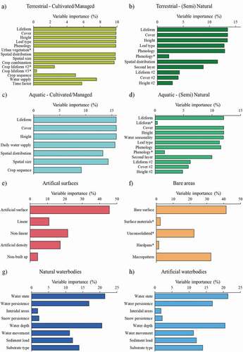
For non-vegetated classes, tier 1 landscape attributes dominated the unique landscape descriptions for artificial surfaces and bare areas, accounting for > 40% of unique descriptions (Figure 3). Water state explains > 20% of descriptors, with water persistence and depth contributing 17% and 21% respectively. Surprisingly, water depth is of greater importance than any tier 2 variables, despite being a tier 3 variable.

For implementing Living Earth and deriving environmental descriptor inputs, variable importance analysis identifies priority inputs for landscape descriptions. For vegetation, deriving lifeform, cover and height are of highest priority. For aquatic vegetation, attributes of edaphic conditions (daily water supply, water seasonality) should be derived subsequently. Spatial information should be the proceeding focus, such as spatial distribution, spatial size and the presence of second strata. For non-vegetated terrestrial areas, priority should be differentiating artificial surface types (i.e. built up, non-built up, linear, non-linear) and bare surface types (i.e. consolidated, non-consolidated, bare rock, hardpans, loose and shifting sands) as this will directly inform proceeding tier attributes. For waterbodies, focus on water state (i.e. water, snow, ice), and subsequently, environmental descriptors of water persistence and water depth should be prioritised.

4. Discussion

This study showcased the fully implemented FAO LCCS-2, Living Earth, optimised for EO application. Living Earth was developed to align with FAIR principles of software and data dissemination as an open-source system intended to utilise free and available EO data. The classification of land cover can be applied to any rasterised spatial data, independent of spatial and temporal resolution, as well as direct functionality with the Open Data Cube. The plugin design of Living Earth allows easy addition of environmental descriptors pertinent to the use case. Living Earth provides a framework for standardised, globally applicable and comparable land cover classification to support EO4SDGs. To aid nations in adopting Living Earth for SDG target setting and reporting, key environmental descriptors were identified to direct resource allocation so that the most important input data are generated in order of ease and priority. Living Earth has been implemented in Australia and Wales (UK) and will be examined here to provide a roadmap for both nations as well as indicative examples for others reporting on SDGs.

4.1. Living Earth: LCCS-2 optimised for EO

The FAO LCCS-2 provides a consistent and easily interpretable semantic framework for global application, describing approximately 12,000 variations in landscape types. However, there was a substantial need to modify the LCCS-2 to optimise its use for EO inputs and subsequent production of spatially explicit maps. Key modifications needed for Living Earth significantly increased the number of unique landscape descriptions, which approximated 573,307 (almost 50 times more). These included vegetation stratification based on height, the inclusion of height and cover in cultivated/managed taxonomies, and moderate relaxation of hierarchical dependencies with unique classification descriptions in order to provide valid LCCS-2 outputs with limited data inputs. The pronounced increase in unique landscape descriptions occurred because of hierarchical attribution of landscape descriptions at level 4, whereby modifying key classes in the hierarchy increased unique class outputs several fold. For example, the addition of cover and height descriptions to the cultivated/managed classes at tier 1 effectively increased the number of unique output classes of cultivated/managed LCCS-2 classes by 45 times (5 cover categories, 9 height categories).

Modifications from LCCS-2 were considered with two criteria; is the modification a) necessary for EO implementation or b) utilising EO data to enhance landscape descriptions? For example, vegetated categories in LCCS-2 require lifeform as a prerequisite for attribution of vegetation cover and height. However, the generation of vegetation cover and height from EO is more accessible than lifeform at a range of spatial scales. Vegetation cover and height can be measured directly using EO (Lang et al., 2021; Liao, Van Dijk, He, Larraondo, & Scarth, 2020; Los et al., 2012; Potapov et al., 2021), however lifeform derivatives often requires some inference or proxy (often using cover and height, e.g. Scarth, Armston, Lucas, & Bunting, 2019; Schneider et al., 2020). Removing dependencies on lifeform for vegetation cover and height enhanced landscape descriptions provided by LCCS-2 as these environmental descriptors provide sufficient information that is highly desirable. Further modifications to LCCS-2 dependencies were carefully considered to ensure LCCS-2 semantics and taxonomic framework were not undermined. Dependencies that were clearly required to give meaningful context to additional descriptors, that would otherwise be unhelpful when interpreted by an end user, were not altered. For example, spatial distribution requires lifeform, cover and height to give context to why spatial heterogeneity may be important, such as fragmentation of a woodland over time.

4.2. Key environmental descriptors

Identifying key environmental descriptors for Living Earth is helpful for resource allocation and provides a clear pathway for implementation. Output land cover classes in Living Earth are predefined by combining inputs layers, therefore allowing users to focus on generating the most useful layer required as an input. The interchange of input layers, as a function of increased accuracy or precision, enables very effective ongoing maintenance and implementation of the land cover system, as landscape descriptors are not altered from the previous implementation, rather just improved. This facilitates reliable land cover comparisons through space and time, accommodating (and benefitting from) the latest technological and/or computational advances. Key environmental descriptors identified in this study provide specific guidance for users and nations as a pathway for implementation. These priorities will likely be the priorities for diverse and complex landscapes globally, however national implementations may require shifted priorities as appropriate to the landscape.

The natural landscape, particularly vegetated classes, present the most diverse landscape descriptions, accounting for > 99% of all unique descriptors in Living Earth. Generation of tier 1 inputs for vegetated systems should be prioritised (i.e. lifeform, cover and height). Lifeform is a category that can be challenging to generate from EO data, particularly beyond the classes of woody and herbaceous (i.e. trees, shrubs, forbs, graminoids, lichens and/or mosses). For this, a number of methods have been used to generate the categories, including well-developed machine learning approaches (e.g. Vegetation Fractional Cover, Gill et al., 2017; Hill & Guerschman, 2020; Woody Cover Fraction, Liao et al., 2020), or inherent qualities of sensors such as C-band backscatter characteristics (Planque et al., 2021). However, based on the FAO LCCS definitions of lifeform, the best approach is to use continuous raster height products derived from, for example, airborne or spaceborne interferometric SAR or Lidar (e.g. ICESAT or GEDI; Potapov et al., 2021; Schneider et al., 2020; Simard, Pinto, Fisher, & Baccini, 2011) as the provision of a unit measure (i.e. height in metres) provides a defined threshold for differentiating some lifeforms (e.g. trees > 2 m, shrubs < 2 m). Cross tabulations of height and cover also provide the basis for defining forests (e.g. FAO, 2020; Sasaki & Putz, 2009) and generating structural classifications (e.g. Scarth et al., 2019) that can be described according to lifeform, if categorised correctly. We implore users that the generation of lifeform, cover and height of vegetation is the most important metrics for input into Living Earth and this can be achieved using established methods and available EO data.

For non-vegetated classes, resources should focus on categories of water state (i.e. water, snow, ice) and subsequently environmental descriptors of water persistence and water depth. Detection of water bodies is readily achieved using data from optical sensors (e.g. Mueller et al., 2016) and SAR (e.g. Sentinel-1; Huang et al., 2018). In addition, the routine retrieval of identifying waterbodies facilitates time-series approaches to identifying water persistence over time (Krause, Newey, Alger, & Lymburner, 2021; Mueller et al., 2016; Sagar et al., 2017). Water metrics are vital for landscape management globally, and this input to Living Earth represents an important component that should be a priority for implementation.

For terrestrial surfaces, focus should be on differentiating artificial surfaces types (i.e. built up, non-built up, linear, non-linear) and bare surface types (i.e. consolidated, non-consolidated, bare rock, hardpans, loose and shifting sands). However, these can be challenging to classify from EO data, particularly on a routine basis. Differentiation of artificial surface types has been achieved using object-based classifications, with some established methods and demonstrations showing success, albeit varying substantially with sensor type (Chen et al., 2014; Ma et al., 2017; Myint, Gober, Brazel, Grossman-Clarke, & Weng, 2011). For naturally bare areas, several existing products, such as geological and sedimentary mapping, could be utilised. However, routine retrieval of these products is challenging, particularly as spectral properties exploited for geological and sedimentary mapping may not correspond to bare surface types (Post et al., 1994; Roberts, Wilford, & Ghattas, 2019).

4.3. Living Earth for Australia

Australia’s current infrastructure and strategic direction to utilise EO data are highly compatible with Living Earth for mapping the Australian landscape. Digital Earth Australia (DEA) is an ODC instance containing the Australian archive of Landsat data (1987 to present) (Lewis et al., 2017). The ODC framework enables a pixel-based approach, rather than a traditional scene-based approach to analysing Landsat data, providing direct comparison of observations from specific locations acquired at two or more epochs (Dhu et al., 2017). This analytical power provides unprecedented capability for continental-scale analysis at a high temporal frequency and has been used to develop several innovative products (see Bishop-Taylor et al., 2019; Mueller et al., 2016; Roberts, Dunn, & Mueller, 2018; Roberts, Mueller, & McIntyre, 2017; Roberts et al., 2019; Sagar et al., 2017).

Key environmental descriptors required for future development and application of Living Earth for Australia can be identified with knowledge of the unique landscape types and their likely changes, such as impacts of wildfire, identified through vegetation lifeform, cover and height change, as well as flood and drought, through water seasonality and persistence over time. Several environmental descriptors needed to construct the level 4 classes have already been generated at a national level and include broad continuous lifeform (woody, herbaceous) (Liao et al., 2020), vegetation cover via fractional cover metrics (Gill et al., 2017; Hill & Guerschman, 2020), and water persistence for identifying temporal water dynamics in the landscape (Mueller et al., 2016). Australia’s landscape is dominated by natural vegetated areas and retrieval of input for Living Earth should prioritise development of vegetation height and cover metrics through data from spaceborne Lidar (e.g. ICESAT and GEDI). In addition, temporal water dynamics are important for Australian landscape change, and biophysical parameters such as water state, seasonality, and persistence should also be prioritised. Of lesser priority are other environmental descriptors such as leaf type and leaf phenology, as Australia’s native vegetation is dominated by evergreen species.

Australia aims to continue to report on many SDG targets, recently identified through a national review (DFAT, 2018). Several SDG indicators have been identified where the LCCS can provide essential metrics for input (Metternicht et al., 2020), including SDG targets 6.6.1 (change in the extent of water-related ecosystems over time), 11.3.1 (ratio of land consumption rate to population growth rate), and 15.3.1 (proportion of land that is degraded over total land area). Ongoing work has been presented on 15.3.1 (Sims, Barger, Metternicht, & England, 2020; Sims et al., 2019) demonstrating a best practice approach, where reporting on land degradation should also include processes responsible for degradation. Living Earth offers this capacity with its additive attribute of level 4. This allows, for instance, forest degradation to be identified through changes in vegetation lifeform, cover or height rather than high-level change from vegetated to non-vegetated landscapes. This type of approach with multiple lines of evidence for degradation aligns with the interpretation matrix presented in Sims et al. (2020) and good practise guidance (Sims et al., 2019). Current developments of Living Earth for Australia, together with identified key environmental descriptors, have the potential to achieve best practise reporting for the SDG 15.3.1 at a national scale, with spatial and temporal resolutions suitable for measuring and reporting. The adoption of Living Earth for Australia’s SDG reporting would provide a standardised, comparable system for confident estimates of change, aligning currently reported on targets and providing a means to report on additional targets where data sources have not been identified yet.

4.4. Living Earth for Wales (UK)

Wales’ current and emerging EO infrastructure and data sources have provided an ideal opportunity to adopt Living Earth. Land cover mapping using Living Earth compliments the use of freely available EO data to provide an entire open-source framework, coupled with the facilities of high-performance computing (Supercomputing Wales) to analyse, process and classify dense time-series of satellite sensor data. In particular, Sentinel-1 provides a very useful temporal dataset for Wales and the broader UK due to data collection independent of cloud cover. Retrieval of environmental descriptors relevant to Living Earth have recently been demonstrated, including semi-natural vegetation extent (Punalekar et al., 2020), identification of water bodies and water seasonality (Planque et al., 2020), and species-level crop type classification (Planque et al., 2021).

Wales represents a highly modified and complex landscape dominated by pastureland, woodland and urbanised settings (Lucas et al., 2006). Seasonality and episodic events, such as flooding and severe storms, as well as forestry and clear-cutting activities, are common pressures of landscape change in Wales (Planque et al., 2021). Identifying lifeform is of primary importance and facilitates differentiation of environmental descriptors important for major natural resource (e.g. forestry and national park assets) and agricultural land management. Vegetation cover and height are also key environmental descriptors for both major management activities due to seasonality-influenced cover and height changes due to felling and regrowth forestry operations (Punalekar et al., 2020). As the landscape is dominated by deciduous and evergreen broad-leaved and needle-leaved species, leaf type and phenology represent key environmental descriptors alongside vegetation cover and height. The use of dense time-series such as those acquired by the Sentinel-1 enables seasonal variability to be identified, particularly leaf-on and leaf-off vegetation dynamics to be discerned (Lucas et al., 2011). In addition, temporal water dynamics are important in Wales and the broader UK due to the impacts of flooding and severe storms. Environmental descriptors relevant to water state and water persistence in the landscape should be prioritised. Beyond these priorities, descriptors of lesser priority include those relevant to non-vegetated terrestrial landscapes because of the general absence of naturally bare areas, as well as a small proportional change in artificial surface cover over annual time scales.

A recent national voluntary review on SDGs by the UK Office of National Statistics (ONS) identified a major opportunity for increasing geographical disaggregation for SDG indicator reporting (i.e. SDG indicator reporting at local, regional and devolved levels, such as Wales) (HM Government, 2019). This gives greater granularity to identify progress in SDG targets, however, it also requires greater capacity to standardise and collate information. The ONS indicates several current examples being explored with the Ordnance Survey, including 9.1.1 (Proportion of the rural population that is living within two kilometres of an all-season road) and 11.3.1 (Ratio of land consumption rate to population growth rate). Several SDGs indicators that have been shown to have direct applicability to reporting by EO data are still under exploratory processes for determining appropriate spatial and temporal resolution of available data sources. However, the LCCS would provide direct metrics to report on particular indicators, including 15.3.1 (Proportion of land that is degraded over total land area), 6.6.1 (Change in water-use efficiency over time). Several other indicators applicable for EO are already reported on using global or Europe-wide products although these could also be reported on through Living Earth, potentially at higher spatial resolutions and temporal frequencies (e.g. 15.4.2 Mountain Green Cover Index or 15.1.1, Forest area as a proportion of total land area; HM Government, 2019).

4.5. Living Earth supporting SDG reporting for any nation

Earth observation in support of SDGs (EO4SDGs) has been highlighted by several authors recently (Anderson, Ryan, Sonntag, Kavvada, & Friedl, 2017; Avtar, Aggarwal, Kharrazi, Kumar, & Kurniawan, 2020; Dong, Metternicht, Hostert, Fensholt, & Chowdhury, 2019; Scott & Rajabifard, 2017), with at least 29 key indicators able to be reported on directly through EO or indirectly as a supporting measure. Land cover is suggested to be required in some capacity by 31 indicators (Anderson et al., 2017). Of these, 29 enable direct input from EO for their computation, including 6.6.1 (Percentage of change in the extent of water-related ecosystems, 15.1.1 (Forest area as a percentage of total land area), 15.2.1 (Forest cover under sustainable forest management), 15.2.2 (Net permanent forest loss), and 15.3.1 (Percentage of land that is degraded over total land area) (Anderson et al., 2017). All 29 EO-applicable indicators rely on environmental descriptors (Masó, Serral, Domingo-Marimon, & Zabala, 2019) but need to be routinely retrievable, freely available, and comparable over space and time for global reporting strategies (Scott & Rajabifard, 2017). To achieve sustainable development goals through consistent reporting of indicators), we suggest that Living Earth provides a viable and potentially optimal platform for global adoption for EO4SDGs. Living Earth ensures a transparent methodology that allows monitoring to be standardised for all countries with the cooperation of the scientific and political communities – key conclusions from recent reviews (Anderson et al., 2017; Avtar et al., 2020).

Living Earth is highly compatible and complementary with free and open access ARD to provide standardised methods for assessing land cover and land cover change (Dong et al., 2019). The Living Earth software package pairs with readily accessible global EO data and current and emerging national infrastructures for EO monitoring. Apart from the aforementioned examples of Australia and Wales (UK), the continuing development and momentum of the Open Data Cube (ODC) provides an excellent integration with the Living Earth software for generating land cover and land cover change products at relevant spatial and temporal resolutions for measuring and reporting on SDGs. The seamless integration with ODC means that Living Earth can be adopted by any nation utilising ODC for spatial data management and analysis.

5. Conclusion

This study presents Living Earth, an implemented, flexible, optimised FAO LCCS-2, suitable for the classification of land cover in support of SDG target setting and reporting. Living Earth provides a framework for standardised, globally applicable and comparable land cover classification to support EO4SDGs, providing information and knowledge for action, rather than only ARD. We resolve several semantic challenges of LCCS for consistent EO implementation, including modifications to environmental descriptors, inter-dependency within the modular-hierarchical framework, and increased flexibility associated with limited data availability. The Living Earth software package was developed to align with FAIR principles of software and data dissemination, as an open-source system intended to utilise free and available EO data. The plugin design of Living Earth allows easy addition of landscape descriptors pertinent to the use case selected. Key environmental descriptors provide specific guidance for users and nations as a pathway for application to build a successful ongoing and relevant national land cover product.

Acknowledgments

The authors would like to recognise the considerable effort of the Open Data Cube community to provide an analytical framework for scalable land cover mapping. Ben Lewis, Gabrielle Hunt, Cate Kooymans, Sebastien Chognard and Sophia German are thanked for their helpful contributions and thoughts to implementing Living Earth from FAO LCCS-2. This paper was published with the permission of the CEO, Geoscience Australia.

Disclosure statement

No potential conflict of interest was reported by the author(s).

Data availability statement

The Living Earth system is under Apache 2.0 license, available on bitbucket (https://bitbucket.org/au-eoed/livingearth_lccs). Extensive documentation, such as detailed descriptions of FAO LCCS-2 class modifications for EO, is available in the repository. All 573,307 unique landscape descriptor codes and descriptions are provided in supplementary material along with variable importance scores for each environmental descriptor. Any further requests should be made to the corresponding author.

Supplementary material

Supplemental data for this article can be accessed here.

Additional information

Funding

This research has been conducted with the support of Geoscience Australia, through the DEA Land Cover project, and the European Research Development Fund (ERDF) Sêr Cymru II program award (80761-AU-108; Living Wales).

Notes on contributors

Christopher J. Owers

Christopher J. Owers is part of the Quantitative Biodiversity Assessment team at CSIRO exploring habitat condition and environmental change at national and global scales. His work involves developing transformative technology to enable rapid response to ecosystem change for more effective and efficient biodiversity management. Previously he was part the Earth Observation and Ecosystem Dynamics research group at Aberystwyth University, contributing expertise on remote sensing and landscape geomorphology with an emphasis on land monitoring and management. His research interests span environmental science with a passion on using spatial information to identify landscape change.

References

- Anderson, K., Ryan, B., Sonntag, W., Kavvada, A., & Friedl, L. (2017). Earth observation in service of the 2030 agenda for sustainable development. Geo-Spatial Information Science, 20(2), 77–96. doi:https://doi.org/10.1080/10095020.2017.1333230
- Arino, O., Bicheron, P., Achard, F., Latham, J., Witt, R., & Weber, J. L. (2008). GLOBCOVER the most detailed portrait of Earth. ESA Bulletin European Space Agency, 136, 24–31.
- Atyeo, C., & Thackway, R. (2006). Classifying Australian land cover. Canberra, Australia: Bureau of Rural Sciences.
- Avtar, R., Aggarwal, R., Kharrazi, A., Kumar, P., & Kurniawan, T. A. (2020). Utilizing geospatial information to implement SDGs and monitor their progress. Environmental Monitoring and Assessment, 192(1). doi:https://doi.org/10.1007/s10661-019-7996-9
- Berge, M., Moreno, J., Johannessen, J. A., Levelt, P. F., & Hanssen, R. F. (2012). ESA’s sentinel missions in support of Earth system science. Remote Sensing of Environment, 120, 84–90.
- Bicheron, P., Defourny, P., Brockmann, C., Schouten, L., Vancutsem, C., Huc, M., … Arino, O. (2008). Globcover. Toulouse, France: Products Description and Validation Report.
- Bishop-Taylor, R., Sagar, S., Lymburner, L., & Beaman, R. J. (2019). Between the tides: Modelling the elevation of Australia’s exposed intertidal zone at continental scale. Estuarine, Coastal and Shelf Science, 223, 115–128.
- Bontemps, S., Defourny, P., Radoux, J., Van Bogaert, E., Lamarche, C., Achard, F., … Arino, O. 2013. Consistent global land cover maps for climate modelling communities: Current achievements of the ESA Land Cover CCI. ESA Living Planet Symposium, Edinburgh, UK. ESA SP-722-713
- Bossard, M., Feranec, J., & Otahel, J. (2000). CORINE land cover technical guide: addendum 2000. Copenhagen, Denmark: European Environment Agency (EEA).
- Calderón-Loor, M., Hadjikakou, M., & Bryan, B. A. (2021). High-resolution wall-to-wall land-cover mapping and land change assessment for Australia from 1985 to 2015. Remote Sensing of Environment, 252. doi:https://doi.org/10.1016/j.rse.2020.112148
- Chen, J., Chen, J., Liao, A., Cao, X., Chen, L., Chen, X., … Mills, J. (2014). Global land cover mapping at 30m resolution: A POK-based operational approach. ISPRS Journal of Photogrammetry and Remote Sensing, 103, 7–27.
- DESA, U.N. 2016. Transforming our world: The 2030 agenda for sustainable development. Resolution Adopted by the UN General Assembly. https://www.unfpa.org/sites/default/files/resource-pdf/Resolution_A_RES_70_1_EN.pdf. (accessed 12 March 2021).
- DFAT. 2018. Report on the implementation of the sustainable development goals (voluntary national review). Department of Foreign Affairs and Trade, Australia. https://www.dfat.gov.au/sites/default/files/sdg-voluntary-national-review.pdf (accessed 14 January 2021).
- Dhu, T., Dunn, B., Lewis, B., Lymburner, L., Mueller, N., Telfer, E., … Phillips, C. (2017). Digital Earth Australia – unlocking new value from earth observation data. Big Earth Data, 1, 64–74.
- Di Gregorio, A. (2005). Land cover classification system: Classification concepts and user manual, software version 2. Rome: Food and Agriculture Organization of the United Nations.
- Di Gregorio, A. 2016. Land cover classification system user manual, software version 3. Food and Agriculture Organization of the United Nations, Rome. http://www.fao.org/3/i5428e/i5428e.pdf (accessed 1 December 2020).
- Di Gregorio, A., & Jansen, L. J. M. 2000. Land cover classification system – classification concepts and user manual. Food and Agriculture Organization of the United Nations, Rome. http://www.fao.org/3/x0596e/x0596e00.htm (accessed 1 December 2020).
- Dong, J., Metternicht, G., Hostert, P., Fensholt, R., & Chowdhury, R. R. (2019). Remote sensing and geospatial technologies in support of a normative land system science: Status and prospects. Current Opinion in Environmental Sustainability, 38, 44–52.
- EO4SDG. 2020. Earth observations in services of the 2030 agenda for sustainable development. https://earthobservations.org/documents/gwp20_22/eo_for_sustainable_development_goals_ip.pdf (accessed 20 February 2021).
- Estoque, R. C. (2020). A review of the sustainability concept and the state of SDG monitoring using remote sensing. Remote Sensing, 12(11), 1770.
- FAO. 2020. Global forest resources assessment. Guidelines and specifications. FRA 2020 version 1.0. Food and Agriculture Organization of the United Nations http://www.fao.org/3/I8699EN/i8699en.pdf (accessed 12 April 2021).
- Ferreira, B., Iten, M., & Silva, R. G. (2020). Monitoring sustainable development by means of earth observation data and machine learning: A review. Environmental Sciences Europe, 32, 120.
- Franklin, S. E., & Wulder, M. A. (2002). Remote sensing methods in medium spatial resolution satellite data land cover classification of large areas. Progress in Physical Geography, 26(2), 173–205.
- Friedl, M. A., Sulla-Menashe, D., Tan, B., Schneider, A., Ramankutty, N., Sibley, A., & Huang, X. M. (2010). MODIS collection 5 global land cover: Algorithm refinements and characterization of new datasets. Remote Sensing of Environment, 114(1), 168–182. doi:https://doi.org/10.1016/j.rse.2009.08.016
- GDAL/OGR contributors. 2021. GDAL/OGR geospatial data abstraction software library. Open Source Geospatial Foundation. https://gdal.org (accessed 14 April 2021).
- Gill, T., Johansen, K., Phinn, S., Trevithick, R., Scarth, P., & Armston, J. A. (2017). A method for mapping Australian woody vegetation cover by linking continental-scale field data and long-term Landsat time series. International Journal of Remote Sensing, 38, 679–705.
- Gillies, S. 2019. Rasterio: Geospatial raster I/O for python programmers. Mapbox. https://github.com/mapbox/rasterio (accessed 14 April 2021).
- Gillingham, S., & Flood, N. 2014. RIOS. https://github.com/ubarsc/rios (accessed 14 April 2021).
- Gomes, V. C. F., Queiroz, G. R., & Ferreira, K. R. (2020). An overview of platforms for big earth observation data management and analysis. Remote Sensing, 12, 1253.
- Gómez, C., White, J. C., & Wulder, M. A. (2016). Optical remotely sensed time series data for land cover classification: A review. ISPRS Journal of Photogrammetry and Remote Sensing, 116, 55–72.
- Hansen, M., DeFries, R., Townshend, J., & Sohlberg, R. (2000). Global land cover classification at 1 km spatial resolution using a classification tree approach. International Journal of Remote Sensing, 21(6–7), 1331–1364.
- Harris, C. R., Millman, K. J., van der Walt, S. J., Gommers, R., Virtanen, P., Cournapea, D., … Oliphant, T. E. (2020). Array programming with NumPy. Nature, 585(7825), 357–362.
- Hill, M. J., & Guerschman, J. P. (2020). The MODIS global vegetation fractional cover product 2001 – 2018: characteristics of vegetation fractional cover in Grasslands and Savanna Woodlands. Remote Sensing, 12(3), 406. doi:https://doi.org/10.3390/rs12030406
- HM Government. 2019. Voluntary national review of progress towards the sustainable development goals: United Kingdom of Great Britain and Northern Ireland. Department of International Development, UK. https://www.gov.uk/government/publications/uks-voluntary-national-review-of-the-sustainable-development-goals (accessed 1 December 2020).
- Hoyer, S., & Hamman, J. (2017). xarray: N-D labeled arrays and datasets in python. Journal of Open Research Software, 5(1), 10.
- Huang, W., DeVries, B., Huang, C., Lang, M. W., Jones, J. W., Creed, I. F., & Carroll, M. L. (2018). Automated extraction of surface water extent from Sentinel-1 data. Remote Sensing, 10(5), 797.
- Kavvada, A., Metternicht, G., Kerblat, F., Mudau, N., Haldorson, M., Laldaparsad, S., … Chuvieco, E. (2020). Towards delivering on the Sustainable Development Goals using Earth observations. Remote Sensing of Environment, 247, 111930.
- Killough, B. 2018. Overview of the Open data cube initiative. IGARSS IEEE International Geoscience and Remote Sensing Symposium, Valencia, Spain, 8629–8632. doi:https://doi.org/10.1109/IGARSS.2018.8517694
- Killough, B., Siqueira, A., & Dyke, G. 2020. Advancements in the open data cube and analysis ready data - past present and future. IGARSS IEEE International Geoscience and Remote Sensing Symposium, Virtual Symposium.
- Kosmidou, V., Petrou, Z., Bunce, R. G. H., Mücher, C. A., Jongman, R. H. G., Bogers, M. M. B., … Petrou, M. (2014). Harmonization of the Land Cover Classification System (LCCS) with the General Habitat Categories (GHC) classification system. Ecological Indicators, 36, 290–300. doi:https://doi.org/10.1016/j.ecolind.2013.07.025
- Krause, C. E., Newey, V., Alger, M. J., & Lymburner, L. (2021). Mapping and monitoring the multi-decadal dynamics of Australia’s open waterbodies using Landsat. Remote Sensing, 13(8), 1437.
- Lang, N., Kalischek, N., Armston, J., Schindler, K., Dubayah, R., & Wegner, J. D. 2021. Global canopy height estimation with GEDI LIDAR waveforms and Bayesian deep learning. Cornell University. https://arxiv.org/abs/2103.03975
- Latifovic, R., Homer, C., Ressel, R., Pouliot, D., Hossain, N., Colditz, R., … Victoria, A. (2012). North American land change monitoring system. In C. P. Giri (Ed.), Remote sensing of land use and land cover: Principles and applications (Vol. 8, pp. 303–324). Boca Raton, USA: CRC Press.
- Lewis, A., Oliver, S., Lymburner, L., Evans, B., Wyborn, L., Mueller, N., … Wang, L. (2017). The Australian geoscience data cube – foundations and lessons learned. Remote Sensing of Environment, 202, 276–292. doi:https://doi.org/10.1016/j.rse.2017.03.015
- Li, Q., Qiu, C., Ma, L., Schmitt, M., & Zhu, X. X. (2020). Mapping the land cover of Africa at 10 m resolution from multi-source remote sensing data with Google Earth Engine. Remote Sensing, 12(4), 1–22.
- Liao, Z., Van Dijk, A. I. J. M., He, B., Larraondo, P. R., & Scarth, P. F. (2020). Woody vegetation cover, height and biomass at 25-m resolution across Australia derived from multiple site, airborne and satellite observations. International Journal of Applied Earth Observation and Geoinformation, 93, 102209.
- Los, S. O., Rosette, J. A. B., Kljun, N., North, P. R. J., Chasmer, L., Suárez, J. C., … Berni, J. A. J. (2012). Vegetation height and cover fraction between 60° S and 60° N from ICESat GLAS data. Geoscientific Model Development, 5, 413–432.
- Loveland, T., Reed, B., Brown, J., Ohlen, D., Zhu, J., Yang, L., & Merchant, J. (2000). Development of a global land cover characteristics database and IGBP discover from 1-km AVHRR data. International Journal of Remote Sensing, 21(6–7), 1303–1330. doi:https://doi.org/10.1080/014311600210191
- Lucas, R., & Mitchell, A. (2017). Integrated land cover and change classifications. In R. Díaz-Delgado & C. H. Lucas (Eds.), The roles of remote sensing in nature conservation: A practical guide and case studies (pp. 295–308). Charm, Switzerland: Springer International Publishing.
- Lucas, R., Mueller, N., Siggins, A., Owers, C., Clewley, D., Bunting, P., … Metternicht, G. (2019). Land cover mapping using digital earth Australia. Data, 4(4), 143.
- Lucas, R., Otero, V., Kerchove, R. V. D., Lagomasino, D., Satyanarayana, B., Fatoyinbo, T., & Dahdouh‐Guebas, F. (2020). Monitoring matang’s mangroves in Peninsular Malaysia through earth observations: A globally relevant approach. Land Degradation & Development, 32(1), 354–373.
- Lucas, R. M., Medcalf, K., Brown, A., Bunting, P., Breyer, J., Clewley, D., … Blackmore, P. (2011). Updating the Phase 1 habitat map of Wales, UK, using satellite sensor data. ISPRS Journal of Photogrammetry and Remote Sensing, 66(1), 81–102.
- Lucas, R. M., Rowlands, A., Brown, A., & Bunting, P. (2006). Rule-based classification of multi-temporal satellite imagery for habitat and agricultural land cover mapping. ISPRS Journal of Photogrammetry and Remote Sensing, 62(3), 165–185.
- Lymburner, L., Tan, P., Mueller, N., Thackway, R., & Thankappan, M. 2011. The national dynamic land cover dataset - technical report. Record 2011/031. Geoscience Australia, Canberra, Australia. http://www.ga.gov.au/corporate_data/71069/Rec2011_031.pdf (accessed 10 April 2020)
- Ma, L., Li, M., Ma, X., Cheng, L., Du, P., & Liu, Y. (2017). A review of supervised object-based land-cover image classification. ISPRS Journal of Photogrammetry and Remote Sensing, 130, 277–293.
- Masó, J., Serral, I., Domingo-Marimon, C., & Zabala, A. (2019). Earth observations for sustainable development goals monitoring based on essential variables and driver-pressure-state-impact-response indicators. International Journal of Digital Earth, 217–235. doi:https://doi.org/10.1080/17538947.2019.1576787
- Metternicht, G., Mueller, N., & Lucas, R. (2020). Digital earth for sustainable development goals. In H. Guo, M. F. Goodchild, & A. Annoni (Eds.), Manual of Digital Earth, p. 443. Singapore: Springer.
- Mueller, N., Lewis, A., Roberts, D., Ring, S., Melrose, R., Sixsmith, J., … Ip, A. (2016). Water observations from space: Mapping surface water from 25 years of Landsat imagery across Australia. Remote Sensing of Environment, 174, 341–352.
- Myint, S. W., Gober, P., Brazel, A., Grossman-Clarke, S., & Weng, Q. (2011). Per-pixel vs. object-based classification of urban land cover extraction using high spatial resolution imagery. Remote Sensing of Environment, 115(5), 1145–1161.
- Paganini, M., Petiteville, I., Ward, S., Dyke, G., Steventon, M., Harry, J., & Kerblat, F. 2018. Satellite earth observations in support of the sustainable development goals. http://eohandbook.com/sdg/files/CEOS_EOHB_2018_SDG.pdf (accessed 1 June 2020).
- Planque, C., Lucas, R., Punalekar, S., Chognard, S., Hurford, C., Owers, C., … Bunting, P. (2021). National crop mapping using Sentinel-1 time series: A knowledge-based descriptive algorithm. Remote Sensing, 13(5), 846.
- Planque, C., Punalekar, S., Lucas, R., Chognard, S., Owers, C., Clewley, D., … Horton, C. (2020). Living Wales: Automatic and routine environmental monitoring using multisource Earth observation data. SPIE 11534. Earth Resources and Environmental Remote Sensing/GIS Applications, XI, 115340C.
- Post, D. F., Horvath, E. H., Lucas, W. M., White, S. A., Ehasz, M. J., & Batchily, A. K. (1994). Relations between soil color and Landsat reflectance on semiarid rangelands. Soil Science Society of America Journal, 58(6), 1809–1816.
- Potapov, P., Li, X., Hernandez-Serna, A., Tyukavina, A., Hansen, M. C., Kommareddy, A., … Hofton, M. (2021). Mapping global forest canopy height through integration of GEDI and Landsat data. Remote Sensing of Environment, 253, 112165.
- Punalekar, S. M., Planque, C., Poslajko, P., Lucas, R., Chognard, S., Owers, C. J., … Horton, C. (2020). Mapping dominant genus/species types in natural and seminatural landscapes across Wales through application of Sentinel-2 time-series data. SPIE 11528. Remote Sensing for Agriculture, Ecosystems, and Hydrology, XXII, 1152805.
- Roberts, D., Dunn, B., & Mueller, N. 2018. Open data cube products using high-dimensional statistics of time series. IGARSS IEEE International Geoscience and Remote Sensing Symposium, Valencia, Spain, 8647–8650. doi:https://doi.org/10.1109/igarss.2018.8518312
- Roberts, D., Mueller, N., & McIntyre, A. (2017). High-dimensional pixel composites from earth observation time series. IEEE Transactions in Geoscience and Remote Sensing, 99, 1–11.
- Roberts, D., Wilford, J., & Ghattas, O. (2019). Exposed soil and mineral map of the Australian continent revealing the land at its barest. Nature Communications, 10(1), 5297.
- Rogan, J., & Chen, D. (2004). Remote sensing technology for mapping and monitoring land- cover and land-use change. Progress in Planning, 61(4), 301–325.
- Sagar, S., Roberts, D., Bala, B., & Lymburner, L. (2017). Extracting the intertidal extent and topography of the Australian coastline from a 28 year time series of Landsat observations. Remote Sensing of Environment, 195, 153–169.
- Sasaki, N., & Putz, F. E. (2009). Critical need for new definitions of “forest” and “forest degradation” in global climate agreements. Conservation Letters, 2(5), 226–232. doi:https://doi.org/10.1111/j.1755-263X.2009.00067.x
- Scarth, P., Armston, J., Lucas, R., & Bunting, P. (2019). A structural classification of australian vegetation using ICESat/GLAS, ALOS PALSAR, and landsat sensor data. Remote Sensing, 11(2), 147.
- Schneider, F. D., Ferraz, A., Hancock, S., Duncanson, L. I., Dubayah, R. O., Pavlick, R. P., & Schimel, D. S. (2020). Towards mapping the diversity of canopy structure from space with GEDI. Environmental Research Letters, 15(11), 115006.
- Scott, G., & Rajabifard, A. (2017). Sustainable development and geospatial information: A strategic framework for integrating a global policy agenda into national geospatial capabilities. Geo-spatial Information Science, 20(2), 59–76.
- Simard, M., Pinto, N., Fisher, J. B., & Baccini, A. (2011). Mapping forest canopy height globally with spaceborne Lidar. Journal of Geophysical Research, 116(G4). doi:https://doi.org/10.1029/2011JG001708
- Sims, N. C., Barger, N. N., Metternicht, G. I., & England, J. R. (2020). A land degradation interpretation matrix for reporting on UN SDG indicator 15.3.1 and land degradation neutrality. Environmental Science & Policy, 114, 1–6.
- Sims, N. C., England, J. R., Newnham, G. N., Alexander, S., Green, C., Minelli, S., & Held, A. (2019). Developing good practice guidance for estimating land degradation in the context of the United Nations Sustainable Development Goals. Environmental Science & Policy, 92, 349–355.
- UNGA. (2015). United Nations General Assembly. Sustainable Development Goals (SDGs). New York, NY, USA: United Nations.
- UNGA. 2019. United Nations General Assembly SDG Summit. Summary of the President of the General Assembly. United Nations, New York, NY, USA. https://sustainabledevelopment.un.org/content/documents/25200SDG_Summary.pdf (accessed 10 February 2021)
- Venter, Z. S., & Sydenham, M. A. K. (2021). Continental-scale land cover mapping at 10 m resolution over Europe (ELC10). Remote Sensing, 13(12), 2301.
- Wilkinson, M. D., Dumontier, M., Aalbersberg, I. J., Appleton, G., Axton, M., Baak, A., … Mons, B. (2016). Comment: The FAIR Guiding Principles for scientific data management and stewardship. Scientific Data, 3(1), 160018. doi:https://doi.org/10.1038/sdata.2016.18
- Woodcock, C. A., Allen, R., Anderson, M., Belward, A., Blindschadler, R., Cohen, W., … Wynne, R. (2008). Free access to Landsat imagery. Science, 320(5879), 1011–1012.
- Yang, H., Li, S., Chen, J., Zhang, X., & Xu, S. (2017). The standardization and harmonization of land cover classification systems towards harmonized datasets: A review. ISPRS International Journal of Geo-Information, 6(5), 154. doi:https://doi.org/10.3390/ijgi6050154