Intelligent geospatial maritime risk analytics using the Discrete Global Grid System

ABSTRACT

Each year, accidents involving ships result in significant loss of life, environmental pollution and economic losses. The promotion of navigation safety through risk reduction requires methods to assess the spatial distribution of the relative likelihood of occurrence. Yet, such methods necessitate the integration of large volumes of heterogenous datasets which are not well suited to traditional data structures. This paper proposes the use of the Discrete Global Grid System (DGGS) as an efficient and advantageous structure to integrate vessel traffic, metocean, bathymetric, infrastructure and other relevant maritime datasets to predict the occurrence of ship groundings. Massive and heterogenous datasets are well suited for machine learning algorithms and this paper develops a spatial maritime risk model based on a DGGS utilising such an approach. A Random Forest algorithm is developed to predict the frequency and spatial distribution of groundings while achieving an R² of 0.55 and a mean squared error of 0.002. The resulting risk maps are useful for decision-makers in planning the allocation of mitigation measures, targeted to regions with the highest risk. Further work is identified to expand the applications and insights which could be achieved through establishing a DGGS as a global maritime spatial data structure.

KEYWORDS:

• Maritime risk
• Discrete Global Grid System
• big data
• machine learning

1. Introduction

The safety of a navigating vessel is the responsibility of its master, who utilise their substantial experience, training and equipment to safely guide a vessel between ports and through potentially hazardous waterways (IMO, 2004). National administrations and harbour authorities have a duty to ensure the safety of these waterways are assessed, determining whether new risk controls such as pilotage or ship routeing schemes are warranted. Conventionally, this task relies on the judgment and experience of professional navigators, but many have proposed maritime risk analysis as a field of scientific research to complement these efforts (Kulkarni, Goerlandt, Li, Banda, & Kujala, 2020; Lim, Cho, Bora, Biobaku, & Parsaei, 2018). Such methods provide a systematic, evidence-based quantitative assessment of risks, overcoming limitations in expert judgment such as bias or heuristics (Kahneman, 2011; Tetlock, 2005).

The growth of maritime risk analysis as a science is a relatively recent development, emerging in the 1970s with work by Fujii and Tanaka (1971) and Macduff (1974) seen as the catalyst for this paradigm (Baksh, Abbassi, Garaniya, & Khan, 2018; Mazaheri, Montewka, & Kujala, 2013). From this, a significant body of diverse work has developed which have attempted to quantify the likelihood or consequence of an incident (Lim et al., 2018). One of the key reasons for this growth is the increasing availability of data, in particular vessel traffic data which is generated from the Automatic Identification System (AIS). AIS is an automated electronic reporting system that is required on all commercial vessels, and is optionally carried by smaller ones, which transmit information about the geographic location, speed, direction and identification of vessels. It is no coincidence that the significant increase in maritime risk studies since the late 2000s documented by Lim et al. (2018) is mirrored by the substantial increased availability of AIS data around the same time, as shown by Lensu and Goerlandt (2019).

Yet, the presence of navigating vessels is not the only relevant risk factor, with bathymetry, pilotage, weather conditions and a myriad of other spatial factors contributing to potential accidents. Therefore, it would be expected that combining vessel traffic and incident data with other heterogeneous datasets is essential for effective risk assessment, but this is only a relatively recent trend (Kulkarni et al., 2020). This is partly due to inherent processing challenges of combining massive and varied datasets and as a result studies are often limited to small regions, short time periods or simplistic methodologies (EMSA, 2018; Lensu & Goerlandt, 2019). This is a significant limitation in model development due to the relative infrequency of which accidents occur, with even the Dover Straits, one of the busiest waterways in the world having on average only 1.2 collisions each year (MAIB, 2014a). Therefore, computational methods to efficiently integrate significant volumes and varieties of maritime data can lead to more robust models that are scalable to large regions.

To overcome challenges of large data volume and variety, there has been a growing interest in the capabilities of big-data technologies within transportation (Milne & Watling, 2019). Big data processing architectures that are better suited to large and heterogenous data processing problems, such as Apache Spark, have been utilised for handling massive AIS datasets (Filipiak, Strozyna, Wecel, & Abramowicz, 2018; Scully, Young, & Ross, 2019; Wu, Xu, Wang, Wang, & Xu, 2017). However, these studies approach only the “volume” aspect of big data at the expense of the “variety” of datasets. By integrating other datasets, new opportunities and avenues of research are opened, such as machine learning which is a recent trend in risk assessment (Hedge & Rokseth, 2020), but for which there is little work in the maritime domain (Dorsey, Wang, Grabowski, Merrick, & Harrald, 2020; Jin, Shi, Yuen, Xiao, & Li, 2019).

In order to facilitate this work, methods to combine massive and heterogenous spatial datasets are required. Conventionally this is achieved using Cartesian grids of latitude and longitude (Filipiak et al., 2018; Wu et al., 2017), however, this is inherently flawed in representing a spherical globe. In response to this, recent work has developed Discrete Global Grid Systems (DGGS) as a three-dimensional, regularised and uniformly discretized system of cells for multi resolution management of geospatial data. Some have argued that such a system has many advantages, particularly when integrating multiple heterogenous datasets, as is necessary in maritime risk analysis. However, there are few applications of DGGS generally (Robertson, Chaudhuri, Hojati, & Roberts, 2020) and within maritime risk analysis specifically.

This study seeks to answer some of these questions by demonstrating a use case of big spatial data analytics for maritime risk assessment. An analytical framework, built around a DGGS spatial data structure, is developed to integrate significant AIS and historical incident data with numerous heterogenous exploratory variables including weather, bathymetry and location of infrastructure and risk controls. From this, it is demonstrated that such a framework serves as an effective basis for machine learning models to predict accident occurrence, specifically the likelihood of commercial ship groundings across the United States.

This work provides the following key contributions. Firstly, this study demonstrates how numerous different factors related to maritime safety can be obtained, digitised and integrated into maritime risk models, exceeding the scale of previous work. This fulfils a growing interest in the potential applications of integrated maritime datasets (Kulkarni et al., 2020; Lensu & Goerlandt, 2019) by offering a practical and suitable spatial data processing pipeline. Secondly, the use of DGGS in spatial risk assessment is presented and evaluated, of which there are recognised to be few examples (Robertson et al., 2020), demonstrating some clear advantages over traditional data structures. Thirdly, a novel methodology is proposed through which maritime risk can be strategically mapped using machine learning methods. Some have argued that machine learning methods offer significant advantages over more conventional maritime risk analysis methodologies but there are few examples (Adland, Jia, Lode, & Skontorp, 2021; Jin et al., 2019). Finally, there are few examples of big data processing for maritime risk assessment (Lensu & Goerlandt, 2019) and this work provides a framework and dataset through which numerous avenues of further work are possible.

The remainder of this article is organised as follows. Section 2 describes some key previous work on maritime risk assessment, particularly their methods and those that have sought to utilise big data. Section 3 describes the methodological approach taken, including the datasets, spatial framework and methodological steps. Section 4 provides some results and discussion of the aforementioned methods. Finally, the conclusions are presented in Section 5.

2. Data driven maritime risk assessment

2.1. Vessel traffic data

The majority of data driven models that assess the safety of navigation rely principally on AIS data to represent the movements of vessels. Under SOLAS Chapter V (IALA, 2002), AIS is required on all vessels over 300 tonnes on international voyage, all vessels over 500 tonnes not on international voyage and most passenger vessels regardless of size. Some smaller vessels, including pleasure craft and fishing vessels, may choose to fit AIS to increase their visibility to larger vessels and improve safety. AIS includes dynamic data (ship position, speed and course) and static data (ship name and type) that is broadcast at regular intervals of between 2 seconds and 3 minutes depending on the type and activity of the vessel (IALA, 2011).

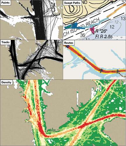
A plethora of different research applications are enabled by AIS including traffic monitoring, emissions modelling, assessing noise/whale strikes amongst many others (Hilliard, Rezaee, & Pelot, 2018; Svanberg, Santen, Horteborn, Holm, & Finnsgard, 2019; Yang, Wu, Wang, Jia, & Li, 2019). To achieve these applications, most commonly, AIS data is processed as a relational database or within a Geographical Information System (GIS). Figure 1 compares the five principal methods through which AIS data is routinely represented in the literature. This includes vector data as points, lines or polygons, or raster data as a density grid. The specific choice of method should reflect both the purpose and scale of analysis. For example, constructing vessel outlines as swept paths are useful to consider the specific circumstances of a transit or incident, but are meaningless at a national scale where ship density would have more utility. These approaches have known limitations which limit their scalability when applied to large datasets (MMO, 2014).

Figure 1. Comparison between representations of AIS data.

The sheer volume and applications of AIS have been argued to fulfil the definitions of “big data” (Abualhaol, Falcon, Abielmona, & Petriu, 2018; Tsou, 2019). Namely:

• Volume – Historical ship traffic data, high resolution metocean data and other data types can be of significant size, exceeding computer memory (Chatzikokolakis, Zissis, Vodas, Spiliopoulos, & Kontopoulos, 2019). Databases need to be able to overcome these challenges and ingest massive quantities of data.

• Velocity – a vessel on transit could be expected to transmit positional data once every 10 seconds, or 8,640 times per day. MarineTraffic, one of the world’s leading commercial enterprises of AIS, record 520 million positions each day across 163,000 unique vessels (MarineTraffic, 2017).

• Variety – 27 message types are transmitted for various purposes, each containing its own attributes (IALA, 2011).

• Veracity – AIS errors are common across a number of attributes. Harati-Mokhtari, Wall, Brooks and Wang (2007) analysed the accuracy of entered AIS information and found that 8% of transmissions were incorrect in some form. Furthermore, AIS can also be faked by generating and transmitting artificial data.

Where the scale of the AIS data under analysis expands, researchers are increasingly turning to big data solutions, offering both greater storage capacity and reduced processing time. Filipiak et al. (2018) utilised Apache Spark to process 310 million vessel positions, calculating statistics and identifying anomalies, demonstrating both significant efficiencies and scalability over conventional methods. Other applications include extracting maritime traffic patterns for anomaly detection (Kontopoulos, Varlamis, & Tserpes, 2020), characterising vessel behaviour near critical infrastructure (Scully et al., 2019), mapping global shipping routes from 21 billion vessel positions (Wu et al., 2017) or presenting novel data models (Widhalm & Dragaschnig, 2020). Few studies have investigated the use of big data processing for use in maritime risk assessment. An exception is the work by Zhang, Meng, and Fwa (2017) which utilised a Hadoop cluster to analyse vessel traffic in Singapore, noting that areas of hot spots of vessel speed coincided with areas where historical incidents had occurred. There is therefore a sparsity of studies that utilise massive AIS datasets for the purposes of maritime risk assessment.

2.2. Integration of vessel traffic and other datasets

Whilst research into AIS analysis has been a significant field of study, understanding the relative likelihood of accident occurrence requires additional datasets to be integrated. For example, wind and wave conditions are required to understand whether adverse conditions contribute to incidents such as container loss or capsize (Adland et al., 2021). Similarly, integration of bathymetry with vessel traffic data is necessary to predict ship groundings. Lensu and Goerlandt (2019) present a structure for integrating AIS data and ice data to investigate ice navigation in the Baltic Sea. Other applications for these integrated datasets include examining tidal offsets of transits at Keelung Harbour (Tsou, 2019) or predicting insurance claims for oceanic voyages (Adland et al., 2021). Yet, given this necessity, it has been recognised that combining vessel traffic, accident data and other datasets is a relatively recent trend (Kulkarni et al., 2020).

Three broad categories of data are required for data driven maritime risk analysis. Firstly, incident data, which represent what happened, where and when. Secondly, a measure of vessel activity against which to benchmark the number of accidents, most commonly AIS data. Finally, integration with other exploratory variables or risk factors which might influence the relative propensity for accidents to occur. Within the literature, a plethora of factors have been proposed and tested, which are summarised in Table 1 (Bye & Aalberg, 2018; Hoorn & Knapp, 2015; Kim, Lee, & Lee, 2019; Kite-Powell, Jin, Jebsen, Papkonstantinou, & Patrikalakis, 1999; Kristiansen, 2005; Mazaheri, Montewka, Kotilainen, Sormunen, & Kujala, 2014; Mazaheri, Montewka, & Kujala, 2016; Olba, Daamen, Vellinga, & Hoogendoorn, 2019b; Olba, Daamen, Vellinga, & Hoogendoorn, 2019a; USCG, 2005; Van Dorp, Harrald, Marrick, & Grabowski, 2008). The relationship between each risk factor and the propensity for accidents is often not straight forward. For example, whilst shallow depth is logically a cause of groundings, ships spend the majority of their time in deep water, actively avoiding areas of shallows, with the exception of the approaches to ports. Therefore, in most locations where there is shallow water, groundings have not occurred. As such a combination of these factors is often necessary to understand the root cause of an incident.

Table 1. Significant causes of maritime accidents.

Category	Cause	Description	Availability of data
Human and Organisational Factors	Inattention and Fatigue	Impacts decision making and position monitoring.	Not directly measurable.
	Bridge Resource Management	Break down of communication onboard results in misunderstandings/poor decision making.	Not directly measurable.
	Communication	Communication between vessels can result in misunderstandings of intentions.	Not directly measurable.
	Position Monitoring	Failure to monitor position can result in vessel off course.	Not directly measurable.
	Training and experience	Inexperience can impact decision making.	Not directly measurable.
	Regulation	Regulatory regime can require enhanced safety regimen onboard.	Not directly measurable.
Vessel and Mechanical Factors	Ship Dimensions and Manoeuvrability Characteristics	Less manoeuvrable vessels are constrained in ability to take evasive action.	AIS static data includes length, offsets and draughts. AIS MMSI/IMO Number can be linked to more detailed vessel databases such as IHS Fairplay.
	Vessel Age	Older vessels may be less well operated or have mechanical issues.	AIS MMSI/IMO Number can be linked to more detailed vessel databases such as IHS Fairplay.
	Vessel Flag State and Safety Regime	Some flag states have greater safety regimes than others.	AIS data includes vessel flag, this can be linked to Paris MoU or Flag of Convenience datasets.
	Vessel Speed	Faster navigating vessels have reduced time to take evasive action.	AIS data includes vessel speed.
External Factors	Traffic Density and Distribution	Higher traffic density increases interactions between vessels.	AIS data analysis to derive density/distribution measures.
	Waterway Geometry	More complex waterways require finer navigation skills than open sea.	Topography/geometry of waterways from charts/digital landmass models.
	Depth	Shallow waterways have more potential for vessels to run aground.	Nautical charts (Paper/ENC), digital bathymetry models.
	Weather (Visibility, wave, ice, darkness etc.)	Wind and waves can overwhelm/capsize a vessel or offset the vessel from its intended course. Visibility impacts hazard perception.	Earth observation datasets, time of transit, ice charts.
	Hydrodynamic Effects (E.g. Tidal, Bank Effect)	Impacts course-keeping ability in constrained waters.	Tidal atlases, hydrodynamic models.
	Support Availability (VTS, Tugs, TSS, Pilotage, Aids to Navigation etc.)	Risk controls can monitor/manage passage safely or respond quickly following a mechanical failure.	Nautical charts, port directions.

Not all recognised relevant risk factors can be easily integrated into data driven risk assessments. The inclusion of human and organisational factors is important due to the significance of these factors in the causation of maritime accidents. Yet, such factors are inherently difficult to implement into risk models. Attempting to quantify the level of alertness of a bridge team using data alone, without access to observations of the bridge environment, is if not impossible, beset with challenges. For example, fatigue of a watch keeper has caused numerous accidents (MAIB, 2014b), yet without monitoring the individual onboard, there is little opportunity for directly measuring this factor. One method to represent this is probabilistically using Bayesian Networks to differentiate the safety performance of crews, vessels or companies (Hanninen, 2014), but the state of this feature is not directly observable. A coastal state, coastguard or port would have no way of discerning which ship in their waters is more at risk of fatigue than others.

Some factors can be more easily represented, such as the weather conditions which can integrate with numerous earth observation datasets available to researchers. Others need to be derived or calculated, such as waterway complexity. One method proposed to represent this is through semi-structured interviews with expert navigators to rate the relative difficulty, such as conducted by Mazaheri et al. (2014). Yet, such an approach has clear limitations when attempting to scale it to national or international study areas. Given these challenges, there are relatively few studies that combine multiple heterogenous datasets for predicting maritime risk. Furthermore, such studies require a consistent and standardised spatial data structure into which each dataset can be effectively integrated.

2.3. Managing spatial data and the DGGS

As the world is inherently continuous there are an infinite number of locations at multiple resolutions. Digital representations must reduce this complexity through the use of generalisations or approximations. Conducting spatial analysis requires a data structure which has global extents into which data can be effectively binned, most commonly some form of tessellation into a finite number of discrete elements. By using this approach, complex and heterogenous datasets can be grouped into local spatial objects, through which more traditional statistical models can be applied. This reduces the complexity of the analytical problem and is therefore more scalable to big data problems. Such an approach has been termed as a form of “congruent geography” (Goodchild, 2018).

Conventionally, spatial models in maritime risk analysis have utilised cartesian grid systems with fixed x-y dimensions (Filipiak et al., 2018; Wu et al., 2017). For example, a risk study of Australian waters utilised a regular 1 nm grid (DNV, 2013) whilst another for Washington State USA utilised a 0.5 nm grid (Van Dorp & Merrick, 2014). However, such a structure attempts to map a regular lattice onto a spherical globe, inevitably introducing a number of distortions in cell size and shape that could limit the validity of analysis (Battersby, Stebe, & Finn, 2016). These may be significant enough to distort results and correlations in maritime risk analysis through the Modifiable Areal Unit Problem (MAUP) if not properly recognised (Openshaw, 1977; Rawson, Sabeur, & Correndo, 2019). It has been demonstrated that by changing the resolution when conducting maritime risk analysis, a significant variation in correlations and accident rates can be provided (Rawson & Brito, 2021). Alternatively, some studies utilise non-aggregated data as ship positions, but this can have significant computational challenges unless some downsampling is undertaken (Adland et al., 2021).

To overcome this, DGGS have been proposed as a spatial reference system that uses a hierarchical tessellation of equal-area cells to manage and present geospatial datasets. Whilst a Cartesian grid could be described as DGGS (Barnes, 2019), the term is more commonly applied to base solids of triangles and hexagons (Sahr, White, & Kimerling, 2003). This approach increased in popularity in the 1990s with efforts focussed at developing a Digital Earth for undertaking and representing spatial analysis (Goodchild, 2000). A DGGS, therefore can be constructed from platonic solids, and partitioned into ever smaller grids. DGGS has also been adopted by the Open Geospatial Consortium, where its standard specifications have been developed and internationally approved (Purss et al., 2019).

DGGS are typically described by their base polyhedron, transformation from spherical to planar face and hierarchical spatial partitioning method. This latter aspect includes the aperture of the system, the ratio of shapes from one resolution to the next resolution (Sahr et al., 2003). For example, an ISEA3H system describes an Icosahedral Snyder Equal Area projection using hexagonal grids with aperture 3. Whilst DGGS can use many platonic shapes (Sahr et al., 2003), many propose that a hexagonal base model exhibits several key advantages. These include their more compact topology, uniformly high symmetry and uniform adjacency between adjacent cells. The more consistent cell area, distance between neighbouring cells and low perimeter to area ratio allows for less distortion when used for spatial statistics (Birch, Oom, & Beecham, 2007). Furthermore, hexagons have numerous visual properties over square grids, such as reduced ambiguity at edges rather than corners, a less regular structure which can be distracting and alignment on an additional axis (Barnes, 2019; Birch et al., 2007).

A number of DGGS packages have been developed. These include rHealPIX (Gibb, 2016), OpenEAGGR (Riskaware, 2017), DGGRID (Barnes, 2016) and H3 (Uber, 2018). These packages allow for configuration of the types, resolution and aperture of the desired grid. There are few examples of these DGGS implementations within published research and projects (Robertson et al., 2020). Purss et al. (2019) discussed a few proposed initiatives that sought to integrate DGGS within big data projects, albeit at an early stage. Some examples include Robertson et al. (2020) use of DGGS to model wildfires, and Jendryke and McClure (2019) spatial analysis of crime data. However, as yet there is little consideration of the relative merits of DGGS for maritime risk studies, and therefore this warrants further attention.

3. Methodology and datasets

3.1. Framework

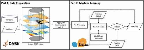
In order to demonstrate the suitability of DGGS as a spatial data structure for maritime risk analysis, this study seeks to predict the frequency of ship grounding across the United States using machine learning. A 2-step framework is proposed (Figure 2). Firstly, numerous exploratory datasets are integrated using a DGGS and summarised using the python library Dask. Secondly, a supervised regression machine learning approach is utilised to predict the frequency of ship groundings within each DGGS cell.

Figure 2. Intelligent geospatial ship grounding model framework.

3.2. Part 1: data preparation

Given the variety of datasets required in this study, a common spatial data framework is required to enable integration and a DGGS is proposed to achieve this. Whilst numerous DGGS packages are available in various languages, as part of the EU Horizon 2020 SEDNA project, the University of Southampton developed a python library that implemented the DGGRID R library (Barnes, 2016), called dggridpy (Correndo, 2019). The package enables DGGS cells to be constructed at varying resolutions, and spatial data indexed. A DGGS was constructed at resolution 7 (3,116 km² area) using a hexagonal ISEA4H DGGS, accounting for approximately 22,000 grid cells across the study area.

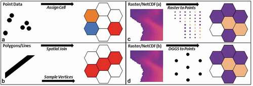
In order to integrate the different datasets into the DGGS, several methods were required and are described in Figure 3. Firstly, point or comma separated value type data, such as vessel positions and incident locations, can be assigned a cell index number from the latitude and longitude using native indexing methods (Figure 3a). Secondly, vector spatial datasets such as polygons or lines can be converted by either writing the DGGS cells as polygons and performing a spatial join or sampling the data centroids as points and then indexing using the conventional method (Figure 3b). Thirdly, raster or NetCDF datasets can be converted by sampling the raster surface with centroids per cell and then assigning a DGGS cell id, before aggregating (through for example averaging) into a single DGGS cell value (Figure 3c). Alternatively, the centroids of the DGGS cells are identified and the corresponding value of that raster cell extracted (Figure 3d). There are strengths and weaknesses in each of these latter methods relating to rasters. For example, if the requirement were to assign depth values within a cell, extracting the raster values of the DGGS cell centroids would be relatively fast. However, if the requirement was to calculate the average depth of the cell it would be necessary to aggregate all of the raster cell values within the DGGS cell.

Figure 3. Methods of assigning DGGS cells to geospatial data.

To support this aggregation, particularly given the significant vessel traffic data which exceeds 170GB, the python library Dask was utilised. Dask supports parallel computing through dynamic task scheduling and extended capability collections such as Panda’s dataframes. A Dask dataframe is a row-wise partition of a Panda’s dataframe such that each partition can be loaded into memory on-demand. A key advantage of Dask over other solutions such as Apache Spark, is the relative similarity and portability of existing python code using standard libraries into Dask. Whilst Spark supports python operations through PySpark, Dask requires minimal conversion of existing code. In addition, Dask also has good scalability, whilst maintaining functionality on a single machine.

3.2.1. Incident data

Under the Code of Federal Regulations 46 CFR 4.03/4.05, any marine casualty or accident occurring with US navigable waters, including grounding, collision, allision or flooding, shall be reported to the Coast Guard. A database of these incidents from 2002 to July 2015 is available specifically for use by researchers. The dataset contains 132,717 incidents. In addition, given the proximity of Canadian waters, data from the Transportation Safety Board of Canada for 1995–2020 was supplemented, accounting for 81,000 records.

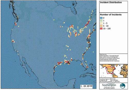
The 200,000 accidents from the combined US and Canadian databases were filtered based on their accident type and vessel types to commercial ship groundings. Several authors have reported issues with the quality of accident data (Mazaheri et al., 2014), and a manual check was made of several groundings that were reported in deep water and omitted as appropriate. Each accident can then be assigned the DGGS cell given the recorded latitude and longitude, with a total of 1,307 groundings. The annual grounding frequency within each DGGS can then be calculated (Figure 4).

Figure 4. Ship grounding accident distribution.

3.2.2. Vessel traffic data

Marine Cadastre, a joint project by the Bureau of Ocean Management and the National Oceanic Atmospheric Administration (NOAA), publish AIS data collected from the US Coast Guard’s national network of AIS receivers. All AIS data for the year 2018 was extracted, approximately 2.5 billion vessel positions.

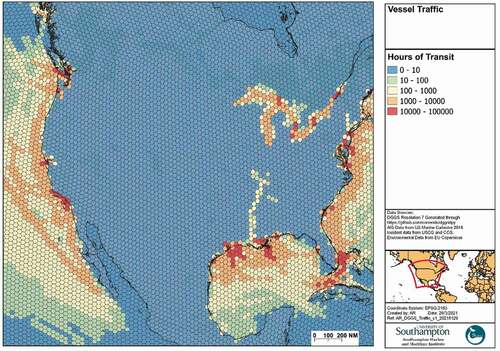
AIS data is broadcast at variable intervals based on the vessel type, speed and behaviour (IALA, 2002, 2011). Therefore, to provide an accurate measure of duration, interpolation of the data to standardised fixed intervals is necessary. Figure 5 describes the workflow to achieve this. Firstly, the extracted data was queried to filter the data to dry cargo and liquid tanker commercial vessels using the ship attributes. Secondly, to remove stationary vessels a filter is applied where the speed is less than 0.5 knots. Thirdly, the data is sorted by MMSI number and timestamp and a loop used to generate a Trip ID number. A Trip is defined as the continuous navigation of one vessel such that the subsequent time between positions is not greater than one hour, at this point it is considered that the tracking of the vessel is lost, and no further interpolation of the vessel is conducted. From this, each trip is then resampled to one-minute intervals and interpolated using the pandas resample and interpolate methods. The data can then be aggregated within each DGGS cell to show the annual hours of commercial vessel transit across the study area (Figure 6).

Figure 5. AIS data processing overview.

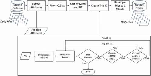
Figure 6. Vessel traffic data.

3.2.3. Bathymetric and topographic data

Bathymetric data was available from NOAA’s National Center’s for Environmental Information’s ETOPO1 Global Relief model. The model provides 1 arc-minute global relief data in netCDF format at WGS84 datum. The average depth within each DGGS cell was then calculated (Figure 7). The high resolution GADM world landmass shapefile was utilised to determine the presence or absence of shore. In addition, a Euclidean Distance calculation was performed to generate a raster map of the study area at 500 m resolution which determine the closest distance to that shoreline. The distance from shore of the centroid of each DGGS cell can then be calculated (Figure 7).

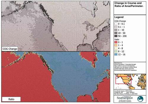
Within Table 1 it was identified that some risk factors for ship accidents relate to the difficulty or complexity of navigating a waterway (Mazaheri et al., 2014). To represent this, two measures were derived (Figure 8). Firstly, the AIS data was filtered to transiting vessels with speeds over 5 knots, and the course changes between each subsequent position calculated and averaged across all transits through that cell. This measure identifies locations with channels that require significant course changes and may be described as more navigationally complex. Secondly, where a DGGS cell intersected the land, the ratio of cell area to cell perimeter was calculated. Cells with a high ratio suggest that the coastline is varied, requiring greater navigational precision.

Figure 7. Bathymetric and topographic datasets.

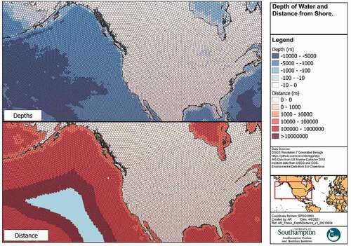
Figure 8. Navigational complexity.

3.2.4. MetOcean data

Metocean data was extracted from the EU Copernicus Marine Environmental Monitoring Service, available in NetCDF format:

• Wind speeds – WIND_GLO_WIND_L4_REP_OBSERVATIONS_012_006 – contains global six hourly mean wind speeds and directions at 0.25 degree resolution.

• Wave heights – GLOBAL_REANALYSIS_WAV_001_032 – contains three hourly mean wave heights and wave directions at a 0.2 degree resolution.

• Ice characteristics – METOFFICE-GLO-SST-L4-REP-OBS-SST – contains daily sea surface details including ice and temperature details at 0.05 degree resolution.

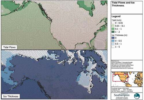
• Tidal flows – GLOBAL-ANALYSIS-FORECAST-PHY-001-024–HOURLY-MERGED-UV – includes hourly surface velocity fields on a 0.05 degree resolution.

In each case, the NetCDF data can be loaded and processed using the xarray python library, to enable standard statistical functions. The 2018 data is aggregated to provide average annual figures for all four metocean conditions (Figures 9 and 10). The data extent is limited to offshore waters and therefore missing values are imputed using the mean coastal values. This data allows characterisation of offshore waters as more exposed to stronger winds and higher wave heights, whilst inshore waters tend to have higher tidal flows. Furthermore, the presence of ice in the northern latitudes can be highlighted.

Figure 9. Wind speeds and wave heights.

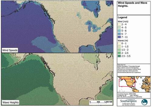
Figure 10. Tidal flows and ice thickness.

3.2.5. Infrastructure and risk controls

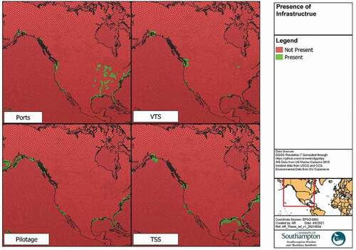
Marine Cadastre and the Homeland Infrastructure Foundation-Level Data Portal provide shapefiles of the locations of key infrastructure such as ports, pilot boarding stations and ship routeing schemes. Given that ports and pilot boarding stations represent specific points, these locations are buffered by 20 nautical miles to account for an approximate area. Such an approach lacks accuracy in specific waterways, but no such dataset of port limits or pilotage regions exists. In addition, the approximate limits of VTS areas are mapped based on CFR legislation and USCG websites. These datasets can then be joined to the DGGS through a spatial intersection (Figure 11).

Figure 11. Presence of infrastructure.

3.2.6. Dataset summary

Table 2 provides summary statistics of the 22,268 DGGS cells and the different features used to develop the model. Each feature is joined utilising the DGGS cell index number.

Table 2. Summary statistics of each DGGS cell.

#	Name	Type	Min	Mean	Max	Description
1	Grounding Frequency/year	Cont.	0	0.004	6.44	Dependent variable
2	Total Vessel Exposure (hours)	Cont.	0	198	72,634	More vessel activity increases likelihood of incidents.
3	Average Wind Speed (m/s)	Cont.	2.0	6.1	10.0	Greater average wind speed reduces ship handling capability.
4	Average Wave Heights (m)	Cont.	0.0	1.24	3.3	Greater average wave size reduces ship handling capability.
5	Average Tidal Flows (m/s)	Cont.	0.00	0.03	1.27	Greater average tidal flow reduces ship handling capability.
6	Average Ice Thickness (m)	Cont.	0.0	0.1	4.8	Greater ice thickness reduces ship maneuverability.
7	Average Depth (m)	Cont.	0	2,524	7,908	Shallower depths increase risk of grounding.
8	Distance from Shore (km)	Cont.	0	3,955	15,000	Closer navigation to shore increases risk of grounding.
9	Navigational Complexity – Topography (Ratio)	Cont.	0.0	4.3	14.0	More complex waterways increase likelihood of grounding.
10	Navigational Complexity – Course Changes (degrees)	Cont.	0	0.31	35.4	More complex waterways increase likelihood of grounding.
11	Presence of TSS (Binary)	Binary	0	0.02	1	Presence of TSS reduces risk of grounding.
12	Presence of Pilot (Binary)	Binary	0	0.02	1	Presence of Pilot reduces risk of grounding.
13	Presence of VTS (Binary)	Binary	0	0.00	1	Presence of VTS reduces risk of grounding.
14	Presence of Key Ports (Binary)	Binary	0	0.02	1	Presence of Ports increases risk of grounding.

3.3. Part 2: machine learning for maritime risk analysis

The resulting dataset consisted of approximately 22,000 DGGS cells that contains aggregated data of 13 features and one target label, namely accident frequency. Few have investigated the application of machine learning to maritime risk assessment (Dorsey et al., 2020; Jin et al., 2019), but such methods enable complex relationships to be represented between multi-dimensional data and therefore should be well suited to navigation safety. The prediction of accident locations y could be framed as a function of the dependent variables x as a form of supervised machine learning such that y = f(x). By training the algorithm on where accidents have occurred, the resulting outputs will indicate regions where the model expects groundings could occur, producing a national risk map to support decision makers.

The machine learning method (Figure 2) consists of several stages. Firstly, the data is split into training and testing datasets with the ratio of 70% to 30%. A Random Forest regression algorithm is then implemented using the library Scikit Learn, with parameter tuning conducted using randomised search with five-fold cross validation, optimising Mean Squared Error (MSE). Random Forest is an ensemble tree-based learning algorithm that has attractive properties such as training speed and robustness when using high-dimensional and unbalanced datasets (Breiman, 2001). Therefore, such a method should be well suited for maritime risk analysis with massive and heterogenous datasets.

Random Forest consists of many decision trees which are a non-parametric supervised learning method that seeks to learn simple decision rules inferred from the data features (Breiman, Freidman, Stone, & Olshen, 1984). Decision trees are constructed in a top-down recursive manner that partitions the data into different groups. At each step, a feature k is split by a threshold value t_k so as to maximise the purity of each subset. The cost function (J) that is optimised can be represented as below, where G and m represent the impurity and number of instances of each subset respectively.

(1) $J\left(k,t_k\right)=\frac{m_{left}}{m}{G}_{left}+\frac{m_{right}}{m}{G}_{right}$(1)

To measure the purity of each node, different measures are available but the gini impurity is utilised here. The impurity (G) is a measure of the proportion of training instances that belong to the same class, where p_i,k is the ratio of class k amongst the training instances in the i-th node.

(2) $G_i=1-\sum _{k=1}^n{p_{i,k}}^2$(2)

Decision trees are prone to overfitting as the data can be continually split until a perfect replication of the training dataset is produced. To overcome this, random forest introduces several features (Breiman, 2001). Firstly, bagging (bootstrap aggregating) involves the training dataset being sampled with replacement. Secondly, randomly selecting attribute variables when splitting the dataset. This leads to decorrelation of each model. For regression problems, the final prediction is the average of each decision tree. In addition, random forest allows for the calculation of the relative importance of each feature in producing the predictions. Feature importance, also referred to as gini importance is calculated by comparing how much the tree nodes that use each feature reduce the impurity on average (Breiman et al., 1984).

4. Results and discussion

4.1. Ship grounding risk model

The results are shown in Figure 12, indicating the spatial variation in ship grounding risk based on the trained Random Forest model. The R² and MSE achieved on the test set are 0.55 and 0.002 respectively. The risk map has many parallels with the map of incident locations shown in Figure 4. For example, high risk areas in the ports such as the Gulf of Mexico, as well as constrained waterways such as the Columbia River, St Lawrence River and Mississippi River are all shown to have high risk. Furthermore, both figures show low risk scores for offshore areas, with deep waters, and inshore areas where there is little vessel traffic. This suggests that the model has good predictive capability at determining the relative risk of grounding across a large area.

Figure 12. Ship grounding risk model.

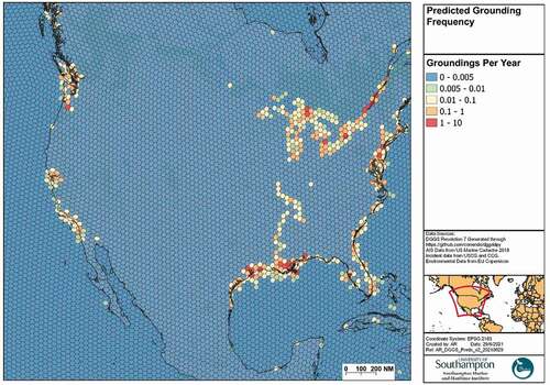
Significantly, the derived risk map also outputs values in regions which have not had historical groundings but are predicted to do so. For example, there have been limited incidents in the Puget Sound region of Washington State, yet this area includes the approaches to major ports of Vancouver and Seattle, with a complex and hazardous waterway. The risk model has identified this area as of concern based on the input features. Therefore, it might warrant further attention by navigation authorities to determine whether additional risk mitigation measures were required. Therefore, without the need for laborious and costly expert input, this approach serves to develop a strategic, high resolution and accurate risk map, to guide decision makers in managing navigation safety.

However, the resulting model has predicted groundings in some locations which appear unlikely. For example, several isolated offshore cells have significant depths of water but are predicted to have a relatively higher risk of grounding than others. A key contributor to this is both the relative low number and underreporting of accidents (Hassel, Asbjornslett, & Hole, 2011; Qu, Meng, & Li, 2012) and also inaccuracies in recording of accident location inherent in many databases. For example, Mazaheri et al. (2014)’s analysis of the HELCOM incident database required the removal of 10% of ship groundings as they had been labelled in areas of deep water. Similarly, Zhang, Sun, Chen, and Cheng (2021) analysed the IMO GISIS database, and accidents are erroneously located in the Sahara. Furthermore, it is notable that only 252 grid cells account for all of the commercial ship groundings and therefore this presents a significant imbalance that is a challenge for supervised machine learning methods (Leevy, Khoshgoftaar, Bauder, & Seliya, 2018).

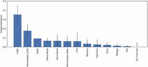
Figure 13 shows the feature importance of the variables used in the ship grounding model. The two most important features for ship groundings are the density of commercial ship traffic and the navigational complexity of the waterway. Vessels are more likely to run aground in areas with many transits, greater numbers of course changes and shallow water. The depth of water is not as significant as might be expected, although there are high correlations between navigational complexity, depth and distance as they are similar measures of the waterway conditions. Metocean conditions might also contribute to ship grounding situations, however, given that the average wind speeds and wave heights are greater further offshore, where the depths are greater, this relationship is not significant. It is notable that many other factors such as presence of risk controls have very little impact upon the prediction of grounding. This is likely reflecting that in areas where depths are shallow and there is significant vessel traffic, pilotage and VTS controls are generally already in place.

The importance of including datasets other than vessel traffic is emphasised by retraining the algorithm utilising only vessel traffic as a single input. An R² of 0.0 was achieved which is significantly less accurate than the model results utilising the other contributory datasets. Furthermore, in comparison to a linear regression algorithm, which achieved an R² of 0.33, Random Forest achieved greater performance.

Figure 13. Feature importance.

4.2. Benefits of DGGS in maritime big data

Maritime risk is a complex and multifaceted problem, and the analysis above demonstrates that it is necessary to integrate multiple datasets to derive accurate and realistic risk maps. This study has utilised DGGS in order to facilitate this integration and several benefits are of note. Firstly, there is a significant computational advantage in utilising aggregated spatial cells rather than coordinates (Purss et al., 2019). For instance, calculations between features within cells are greatly simplified as distance no longer needs to be considered. An infinite number of coordinate pairs can be reduced to a discrete number of cells. As a result, calculations can be performed in parallel with cells distributed across any number of processors, using the unique cell index values. Whilst data-streaming has been performed through Dask, the scaling of the analysis using for instance Apache Spark across multiple nodes would greatly increase processing speed.

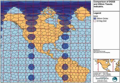
Secondly, DGGS cells are equal area and robust against distortions due to projection systems, which would be significant across large regions such as the United States EEZ. For example, Figure 14 demonstrates the distortion of a Cartesian regular grid of 10-degree cells and DGGS cells. Towards the polar regions, the Tissot’s Indicatrix, with 250 nautical mile geodesic circles shows significant distortion, and whilst the DGGS distorts at the same rate, the regular Cartesian grid cells do not. As a result, the cell area at different latitudes would vary significantly, and may result in spurious statistical relationships as a result of the MAUP. Furthermore, it is possible that machine learning algorithms may become biased by latitude as a result, compromising the predictive capability of such a model. Therefore, normalisation of certain features such as vessel density by cell area may be required to ensure consistency (Eguiluz, Fernandez-Gracia, Irigoien, & Duarte, 2016), but this increases computation and is inefficient. These issues are perhaps exacerbated in the maritime domain, where many projection systems are optimised for national territorial coverage, often placing greatest distortion within the oceans.

Figure 14. Distortion of cell area across study area.

Thirdly, compared to other methods of representing spatial data, such as points, aggregating data into cells enables the inherent representation of uncertainty and data quality (Goodchild, 2018). Where data has high quality and low uncertainty, the resolution can be reduced to a finer scale. Conversely, greater positional uncertainty can be reflected in a coarser resolution of the analysis, such that the data does not exhibit false precision (Robertson et al., 2020). This is particularly important when processing large volumes of data with a wide coverage, inherent to maritime datasets. In traditional analytical approaches, the user manually interacts with the dataset and therefore any significant gaps or errors might be more perceptible. Where the data processing is integrated into automated frameworks, unless the resulting outputs are perceived to be erroneous, these errors might not be identified. Both the AIS and incident datasets have uncertainties that need to be reflected. Within Section 4.1, some limitations with recording of incident data have been highlighted, but more fundamentally, many accident databases are limited to recording positions to degree and minute accuracy, such that positions can be up to one nautical mile from their actual location. AIS positional inaccuracies are typically less significant but do still occur (Iphar, Ray, & Napoli, 2019, 2020). This would be problematic were geospatial analysis conducted on the specific latitude and longitude or at a fine grid size. However, utilising a coarser grid size ensures that the general geographic relationships between features can be captured.

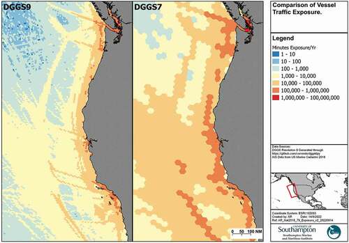
Fourthly, DGGS have inherent capabilities at conducting and visually representing multi-resolution analysis. This might reflect the use-case of the analysis, in this case conducting regional risk analysis warrants courser grid cells than representing individual shipping routes (Figure 15). Maritime trade is inherently multi-resolution and both global shipping patterns and local routes would be difficult to interpret at the same resolution. A multi-resolution DGGS has significant benefit for visualisation of outputs, ensuring that the results are meaningfully interpretable at different scales. Furthermore, this may be to reflect the resolution of the underling individual datasets, for example, vessel traffic data might be aggregated at a higher resolution than metocean data. In addition, some have argued that non-rectangular grids such as hexagons offer advantages for visual interpretation of spatial patterns (Barnes, 2019; Birch et al., 2007).

Figure 15. Comparison of vessel traffic exposure at different DGGS resolutions.

4.3. Towards strategic and real-time intelligent risk analysis

This paper has presented some high-level data handling and analysis of significant volumes and varieties of maritime datasets to inform a ship grounding risk assessment. This has utility to decision-makers for strategic assessment of risk, however, at this stage the work has been limited to only one hazard type and one vessel type. It is likely that the relationship between causal variables will differ between hazard type, for example, metocean conditions would have greater feature importance for predicting capsizes or equipment damage. Further work is planned to explore these relationships. In addition, whilst Random Forest is a popular and sometimes powerful machine learning algorithm, other methods such as deep learning may also be more applicable to this subject and warrant further investigation.

Whilst strategic assessments are useful in managing a waterway and determining the need for risk controls, such as towage or pilotage, there would be significant value in real-time risk assessment. By conducting real-time monitoring of vessel positions and exposure to hazards, coastguards could identify emerging hazardous situations and intervene to prevent accident occurrence or prepare for Search and Rescue. Whilst some pilot projects are ongoing to develop such systems (Dorsey et al., 2020), it is an open area of research. Such a use case would require the inclusion of a temporal dimension, which is omitted by aggregating the datasets described in this paper. Such temporal datasets would be expected to be more correlated with accident conditions than aggregated ones. For example, the wind conditions at the time of an accident/transit are more relevant than aggregated seasonal averages (Adland et al., 2021; Rawson, Brito, Sabeur, & Tran-Thanh, 2021). The importance of temporal factors included in accident models has been shown in other disciplines such as road traffic collisions (Yuan, Zhou, Yang, Tamerius, & Mantilla, 2017). By including this dimension, it would be possible to develop the approach from an aggregated area model to a transit model, whereby the conditions of each individual vessel position can be mined, providing a far greater degree of granularity for risk modelling. Furthermore, an individual vessel model could allow the inclusion of other risk factors that have been argued to correlate to accident propensity, such as vessel type, age or flag state (Bye & Aalberg, 2018). However, there are still research gaps as to how other factors identified in Table 1 such as fatigue and training or experience can be integrated into a quantitative risk model.

Yet, the significant challenge of maritime dataset processing necessary to combine spatiotemporal datasets for vessel traffic and accidents is increased in this approach. Given the advantages of DGGS that are demonstrated within this strategic work, it offers a useful spatial data structure for conducting real-time risk analysis through consistent and efficient data combination and visualisation, whilst accounting for their relative uncertainties. Furthermore, Purss et al. (2019) have proposed that DGGS can be extended through the implementation of datacubes, n-dimensional arrays of values, which would further improve the computational efficiency.

5. Conclusions

The management of navigation safety and prediction of the likelihood of accidents using quantitative techniques poses a number of methodological challenges. Some of these are principally related to the massive size and wide variety of relevant datasets which need to be integrated, processed and analysed in order to draw meaningful insights. This study has provided a framework and discussion of the opportunities that a DGGS offers to support intelligent big-data analytics for maritime risk assessment. By promoting consistent and efficient integration of massive vessel traffic, Earth Observation and other heterogenous datasets, DGGS can enable the development of automated strategic and real-time maritime risk assessments, which would be of significant value for navigational authorities and coastguards to reduce the risk of loss of life and pollution at sea. The derived grounding risk maps enable evidence-based targeting of risk control measures to where they are most required, without the need for laborious, costly and potentially biased expert judgment. Furthermore, the resulting dataset can be used by other researchers for a multitude of other purposes.

Yet, whilst big-data analytics and machine learning methods offers opportunities for improving navigation safety, this work has identified several challenges that require further investigation. In particular, these relate to the representation of human factors in quantitative risk models which could improve the model outputs. However, this study has demonstrated that by combining a DGGS with machine learning algorithms, high-resolution, evidence-based and accurate risk maps can support decision makers in better managing the safety of vessels at sea.

Acknowledgments

This work is partly funded by the University of Southampton’s Marine and Maritime Institute (SMMI) and the European Research Council under the European Union’s Horizon 2020 research and innovation program (grant agreement number: 723526: SEDNA).

Disclosure statement

No potential conflict of interest was reported by the author(s).

Data availability statement

The data that support the findings of this study are available from the corresponding author upon reasonable request. These data were derived from the following resources available in the public domain:

• https://marinecadastre.gov/

• https://marine.copernicus.eu/

• https://www.ngdc.noaa.gov/mgg/global/

• https://gadm.org/data.html

• https://homeport.uscg.mil/Lists/Content/Attachments/211/MISLE DATA.zip

• https://www.tsb.gc.ca/eng/stats/marine/index.html

Aggregated data of the above is available from: https://doi.org/10.7910/DVN/ZZHBFD

Additional information

Funding

This work was supported by the Horizon 2020 [723526]; Southampton Marine and Maritime Institute.

Notes on contributors

Andrew Rawson

Andrew Rawson is a doctoral researcher and maritime consultant specialising in risk analysis and quantitative methods for maritime risk assessment. He has more than a decade experience as project manager and lead analyst of delivering navigation risk studies to ports, offshore developers and governments around the world. In 2018, Andrew commenced doctoral study at the University of Southampton with his thesis entitled “Intelligent Geospatial Analytics for Maritime Risk Assessment”. His principal research interests include the development and application of risk models and machine learning to predict the likelihood of navigation accidents. He has a First-Class degree in Geography from the University of Nottingham. He is a Fellow of the Royal Geographical Society, Member of IMAREST and Associate Member of the Nautical Institute.

Zoheir Sabeur

Zoheir Sabeur is Associate Professor of Data Science at Bournemouth University (2019-present). He is Visiting Professor of Data Science at Colorado School of Mines, Golden, Colorado, USA (2017-present). He was Science Director at School of Electronics and Computer Science, IT Innovation Centre, University of Southampton (2009–2019). He led his big data research team in 27 large projects as Principal Investigator, supported with research grants (totalling £7.0M) and awarded by the European Commission (under FP6, FP7 and H2020), Innovate UK, DSTL, NERC and Industries. Zoheir worked as Director and Head of Research, Marine Information Systems at British Maritime Technology Group Limited (1996–2009). His main research expertise is on Data Science and AI, knowledge extraction, human behaviour and natural processes machine detection and understanding. He has published over 120 papers in scientific journals, conference proceedings and books. He is peer reviewer, member of international scientific committees and editing board of various science and engineering conferences and journals. Zoheir chairs the OGC Digital Global Grid System Specification and Domain Working Groups, and co-chairs the AI and Data Science Task Group at the BDVA. He is Fellow of the British Computer Society, Fellow of IMaREST and Member of the Institute of Physics.

Mario Brito

Mario Brito is an Associate Professor of Risk Analysis and Risk Management. His area of expertise is in risk analysis of extreme events where there is substantial uncertainty with respect to a critical event and historical hard data alone is not sufficient to model the uncertainty. The methods he helped to develop over the years have been applied for supporting decision-making in critical infrastructure or technology operations, including the deployment of autonomous underwater vehicles in extreme environments such as under fast ice or ice shelf. Dr Brito is the leading author of articles published in Risk Analysis, Reliability Engineering and Systems Safety, IEEE Transactions on Engineering Management and Antarctic Science. He was member of the technical panel for international conferences such as PSAM10, AUV2012, UUVS 2012, ESREL 2017-2019 and others. Dr. Brito is the Deputy chair for the Society of Underwater Technology specialist panel on Underwater Robotics and Co-Chair of the European Safety and Reliability Association Committee on Marine and Offshore Technology. He acts as independent reviewer for large ocean infrastructure projects and marine science programmes.

References

- Abualhaol, I. Y., Falcon, R., Abielmona, R. S., & Petriu, E. M. (2018). Mining Port Congestion Indicators from Big AIS Data. International Joint Conference on Neural Networks. Rio de Janeiro, Brazil, 8-13 July 2018.
- Adland, R., Jia, H., Lode, T., & Skontorp, J. (2021). The value of meteorological data in marine risk assessment. Reliability Engineering and System Safety, 209. doi:10.1016/j.ress.2021.107480
- Baksh, A., Abbassi, R., Garaniya, V., & Khan, F. (2018). Marine transportation risk assessment using bayesian network: Application to arctic waters. Ocean Engineering, 159, 422–436.
- Barnes, R. (2016). dggridR: Discrete global grid systems for R [online]. Available at: https://github.com/r-barnes/dggridR. (Accessed 24/ May/2019).
- Barnes, R. (2019). Optimal orientations of discrete global grids and the Poles of Inaccessibility. International Journal of Digital Earth, 13(7), 803–816.
- Battersby, S., Stebe, D., & Finn, M. (2016). Shapes on a Plane: Evaluating the impact of projection distortion on spatial binning. Cartography and Geographic Information Science, 44(5), 410–421.
- Birch, C., Oom, S., & Beecham, J. (2007). Rectangular and hexagonal grids used for observation, experiment and simulation in ecology. Ecological Modelling, 206(3–4), 347–359.
- Breiman, L. (2001). Random Forests. Machine Learning, 45(1), 5–32.
- Breiman, L., Freidman, J., Stone, C., & Olshen, R. (1984). Classification and Regression Trees. New York: Taylor and Francis.
- Bye, R., & Aalberg, A. (2018). Maritime navigation accidents and risk indicators: An exploratory statistical analysis using AIS data and accident reports. Reliability Engineering and System Safety, 176, 174–186.
- Chatzikokolakis, K., Zissis, D., Vodas, M., Spiliopoulos, G., & Kontopoulos, I. (2019). A distributed lightning fast maritime anomaly detection service. Oceans 2019, 17-20 June 2019. Marseillle 10.1109/OCEANSE.2019.8867269
- Correndo, G. (2019). DGGRIDPY Git-hub page [online]. Available at: https://github.com/correndo/dggridpy. (Accessed 22nd May 2020).
- DNV (2013). North east shipping risk assessment. Report No./DNV Reg No. 0/14OFICX-4 Rev 1.
- Dorsey, C., Wang, B., Grabowski, M., Merrick, J., & Harrald, J. (2020). Self-healing databases for predictive risk analytics in safety-critical systems. Journal of Loss Prevention in the Process Industries, 63. doi:10.1016/j.jlp.2019.104014
- Eguiluz, V., Fernandez-Gracia, J., Irigoien, X., & Duarte, C. (2016). A quantitative assessment of Arctic shipping in 2010-2014. Scientific Reports, 6. doi:10.1038/srep30682
- EMSA. (2018). Joint Workshop on Risk Assessment and Response Planning in Europe [online]. Available at: http://www.emsa.europa.eu/workshops-a-events/188-workshops/3246-joint-workshop-on-risk-assessment-response-planning-in-europe.html. (Accessed 17th August 2021).
- Filipiak, D., Strozyna, M., Wecel, K., and Abramowicz, W. (2018). Anomaly Detection in the maritime Domain: Comparison of Traditional and Big Data Approach [online]. Available at:https://www.sto.nato.int/publications/STO%20Meeting%20Proceedings/STO-MP-IST-160/MP-IST-160-S2-5P.pdf(Accessed 17th August 2021)
- Fujii, Y., & Tanaka, R. (1971). Traffic Capacity. Journal of Navigation, 24(4), 543–552.
- Gibb, R. G. (2016). The rHealPIX Discrete Global Grid System. Proceedings of the 9th Symposium of the International Society for Digital Earth, Halifax, Canada, 5-9 October 2015. 10.1088/1755-1315/34/1/012012.
- Goodchild, M. (2000). Discrete Global Grids for Digital Earth. International Conference on Discrete Global Grids. Santa Barbara.
- Goodchild, M. (2018). Reimagining the history of GIS. Annals of GIS, 24(1), 1–8.
- Hanninen, M. (2014). Bayesian networks for maritime traffic accident prevention: Benefits and challenges. Accident Analysis and Prevention, 73, 305–312.
- Harati-Mokhtari, A., Wall, A., Brooks, P., & Wang, J. (2007). Automatic Identification System (AIS): Data reliability and human error implications. Journal of Navigation, 60(3), 373–389. https://www.cambridge.org/core/journals/journal-of-navigation/article/abs/automatic-identification-system-ais-data-reliability-and-human-error-implications/6664900351CB5D9C3FF45F16D96F8832
- Hassel, M., Asbjornslett, B., & Hole, L. (2011). Underreporting of maritime accidents to vessel accident databases. Accident Analysis and Prevention, 43(6), 2053–2063.
- Hedge, J., & Rokseth, B. (2020). Applications of machine learning methods for engineering risk assessment – A Review. Safety Science, 122. doi:10.1016/j.ssci.2019.09.015
- Hilliard, F. M., Rezaee, C., & Pelot, R. (2018). Past, present and future of the satellite-based automatic identification system: Areas of applications (2004-2016). WMU Journal of Maritime Affairs, 17(3), 311–345.
- Hoorn, S., & Knapp, S. (2015). A multi-layered risk exposure assessment approach for the shipping industry. Transportation Research Part A, 78, 21–33.
- IALA. (2002). IALA Guidelines on the Universal Automatic Identification System (AIS). Volume 1, Part II – Technical Issues (Edition 1.1 ed.). France: IALA.
- IALA. (2011). IALA Guideline No 1082 on an Overview of AIS (Edition 1 ed.). France: IALA.
- IMO. (2004). International Convention for the Safety of Life at Sea. London: IMO.
- Iphar, C., Ray, C., & Napoli, A. (2019). Uses and misuses of the automatic identification system. Oceans 2019, 17-20 June 2019. Marseille 10.1109/OCEANSE.2019.8867559
- Iphar, C., Ray, C., & Napoli, A. (2020). Data integrity assessment for maritime anomaly detection. Expert Systems with Applications, 147. doi:10.1016/j.eswa.2020.113219
- Jendryke, M., & McClure, S. (2019). Mapping crime – Hate crimes and hate groups in the USA: A Spatial analysis with gridded data. Applied Geography, 111. doi:10.1016/j.apgeog.2019.102072
- Jin, M., Shi, W., Yuen, K., Xiao, Y., & Li, K. (2019). Oil tanker risks on the marine environment: An empirical study and policy implications. Marine Policy, 108. doi:10.1016/j.marpol.2019.103655
- Kahneman, D. (2011). Thinking, Fast and Slow. London: Penguin.
- Kim, I., Lee, H., & Lee, D. (2019). Development of a new tool for objective risk assessment and comparative analysis at coastal waters. Journal of International Maritime Safety, Environmental Affairs and Shipping, 2(2), 58–66.
- Kite-Powell, H., Jin, D., Jebsen, J., Papkonstantinou, V., & Patrikalakis, N. (1999). Investigation of potential risk factors for groundings of commercial vessels in U.S. Ports. International Journal of Offshore and Polar Engineering, 9, 16-21.
- Kontopoulos, I., Varlamis, I., & Tserpes, K. (2020). A Distributed framework for extracting maritime traffic patterns. International Journal of Geographical Information Science, 35(4), 767–792.
- Kristiansen, S. (2005). Maritime Transportation Safety Management and Risk Analysis. Oxford: Routledge.
- Kulkarni, K., Goerlandt, F., Li, J., Banda, O., & Kujala, P. (2020). Preventing shipping accidents: Past, present and future of waterway risk management with Baltic Sea focus. Safety Science, 129. doi:10.1016/j.ssci.2020.104798
- Leevy, J., Khoshgoftaar, T., Bauder, R., & Seliya, N. (2018). A survey on addressing high-class imbalance in big data. Journal of Big Data, 5(1), 42.
- Lensu, M., & Goerlandt, F. (2019). Big maritime data for the Baltic Sea with a focus on the winter navigation system. Marine Policy, 104, 53–65.
- Lim, G., Cho, J., Bora, S., Biobaku, T., & Parsaei, H. (2018). Models and computational algorithms for maritime risk analysis: A review. Annals of Operational Research, 271(2), 765–786.
- Macduff, T. (1974). Probability of vessel collisions. Ocean Industry, 9, 144–148.
- MAIB. (2014a). Report on the investigation of the collision between Paula C and Darya Gayatri in the South-west lane of the Dover Traffic Separation Scheme on 11 December 2013. Report No 25/2014.
- MAIB. (2014b). Report on the investigation of the grounding of Danio off Longstone, Farne Islands, England on 16 March 2013. Report No 8/2014.
- MarineTraffic. (2017). Marine Traffic: 2007-2017. [online]. Available at: https://issuu.com/marinetraffic/docs/marinetraffic_issueone. (Accessed 19/ April/2019).
- Mazaheri, A., Montewka, J., Kotilainen, P., Sormunen, O. E., & Kujala, P. (2014). Assessing grounding frequency using ship traffic and waterway complexity. Journal of Navigation, 68(1), 89–106.
- Mazaheri, A., Montewka, J., & Kujala, P. (2013). Correlation between the ship grounding accident and the ship traffic – a case study based on the statistics of the gulf of finland. TransNav: International Journal on Marine Navigation and Safety of Sea Transportation, 7(1), 119–124.
- Mazaheri, A., Montewka, J., & Kujala, P. (2016). Towards an evidence-based probabilistic risk model for ship-grounding accidents. Safety Science, 86, 195–210.
- Milne, D., & Watling, D. (2019). Big data and understanding change in the context of planning transport systems. Journal of Transport Geography, 76, 235–244.
- MMO (2014). Mapping UK Shipping Density and Routes Technical Annex: 1066. [online]. Available at: https://assets.publishing.service.gov.uk/government/uploads/system/uploads/attachment_data/file/317771/1066-annex.pdf. (Accessed 19/ 04/2019).
- Olba, X., Daamen, W., Vellinga, T., & Hoogendoorn, S. (2019a). Multi-criteria evaluation of vessel traffic for port assessment: A case study of the Port of Rotterdam. Case Studies on Transport Policy, 7(4), 871–881.
- Olba, X., Daamen, W. V., Vellinga, T., & Hoogendoorn, S. (2019b). Risk assessment methodology for vessel traffic in ports by defining the nautical port risk index. Journal of Marine Science and Engineering, 8. doi:10.3390/jmse8010010
- Openshaw, S. (1977). Optimal zoning systems for spatial interaction models. Environment & Planning A, 9(2), 169–184.
- Purss, M., Peterson, P., Strobl, P., Dow, C., Sabeur, Z., Gibb, R., & Ben, J. (2019). Datacubes – A discrete global grid systems perspective. Cartographica: The International Journal for Geographic Information and Geovisualisation, 54(1), 63–71.
- Qu, X., Meng, Q., & Li, S. (2012). Analyses and Implications of Accidents in Singapore Strait. Transportation Research Record: Journal of the Transportation Research Board, 2273(1), 106–111.
- Rawson, A., Sabeur, Z., & Correndo, G. (2019) Spatial challenges of maritime risk analysis using big data. S. C. Guedes (ed.) In Proceedings of the 8th International Conference on Collision and Grounding of Ships and Offshore Structures (ICCGS 2019), Lisbon, Portugal, (21st to 23rd October 2019). vol. 4, CRC Press/Balkema. pp. 275–283.
- Rawson, A., & Brito, M. (2021). A critique of the use of domain analysis for spatial collision risk assessment. Ocean Engineering, 219, 108259.
- Rawson, A., Brito, M., Sabeur, Z., & Tran-Thanh, L. (2021). A machine learning approach for monitoring ship safety in extreme weather events. Safety Science, 141, 105336.
- Riskaware (2017). The OpenEAGGR software library on Github [online]. Available at: https://github.com/riskaware-ltd/open-eaggr/. (Accessed 24/ May/2019).
- Robertson, C., Chaudhuri, C., Hojati, M., & Roberts, S. (2020). An integrated environmental analytics system (IDEAS) based on a DGGS. ISPRS Journal of Photogrammetry and Remote Sensing, 162, 214–228.
- Sahr, K. M., White, D., & Kimerling, A. J. (2003). Geodesic discrete global grid systems. Cartography and Geographic Information Science, 30(2), 121–134.
- Scully, B., Young, D., & Ross, J. (2019). Mining marine vessel AIS data to inform coastal structure management. Journal of Waterway, Port, Coastal, Ocean Engineering, 146, 2.
- Svanberg, M., Santen, V., Horteborn, A., Holm, H., & Finnsgard, C. (2019). AIS in maritime research. Marine Policy, 106. 10.1016/j.marpol.2019.103520
- Tetlock, P. (2005). Expert Political Judgement: How Good is it? How Can we Know? Princeton: Princeton University Press.
- Tsou, M. (2019). Big data analytics of safety assessment for a port of entry: A case study in Keelung Harbour. Proceedings of the Institute of Mechanical Engineers Part M: Journal of Engineering for the Maritime Environment, 233, pp. 1260–1275.
- Uber. (2018). Hexagonal hierarchical geospatial indexing system [online]. Available at: https://github.com/uber/h3. (Accessed 24/ May/2019).
- USCG. (2005). Ports and Waterways Safety Assessment Workshop Guide [online]. Available at: https://www.navcen.uscg.gov/?pageName=pawsaGuide. (Accessed 21st May 2020).
- Van Dorp, J., & Merrick, J. (2014). VTRA 2010 [online]. Available at:https://www2.seas.gwu.edu/~dorpjr/tab4/publications_VTRA_Update_Reports.html (Accessed 17th August 2021)
- Van Dorp, J. R., Harrald, J. R., Marrick, J. R. W., & Grabowski, M. (2008). VTRA: Technical Appendix D: Expert Judgement Elicitation. [online]. Available at: https://www2.seas.gwu.edu/~dorpjr/VTRA/FINAL%20REPORT/083108/VTRA%20REPORT%20-%20Appendix%20D%20083108.pdf. (Accessed 19/ 04/2019).
- Widhalm, G. A., & Dragaschnig, M. (2020). The M3 massive movement model: A distributed incrementally updatable solution for big movement data exploration. International Journal of Geographical Information Science, 34(2), 2517–2540.
- Wu, L., Xu, Y., Wang, Q., Wang, F., & Xu, Z. (2017). Mapping global shipping density from AIS data. Journal of Navigation, 70(1), 67–81.
- Yang, D., Wu, L., Wang, S., Jia, H., & Li, K. (2019). How big data enriches maritime research – A critical review of Automatic Identification System (AIS) data applications. Transport Reviews, 39(6), 755–773.
- Yuan, Z., Zhou, X., Yang, T., Tamerius, J., & Mantilla, R. (2017). Predicting traffic accidents through heterogeneous urban data: A case study. 23rd ACM SIGKDD Conference on Knowledge Discovery and Data Mining, Halifax. 10.1145/3347146.3359078.
- Zhang, L., Meng, Q., & Fwa, T. (2017). Big AIS data based spatial-temporal analyses of ship traffic in Singapore port waters. Transportation Research Part E, 129, 287–304.
- Zhang, Y., Sun, X., Chen, J., & Cheng, C. (2021). Spatial patterns and characteristics of global maritime accidents. Reliability Engineering and System Safety, 206. 10.1016/j.ress.2020.107310