Evaluation of county-level poverty alleviation progress by deep learning and satellite observations

ABSTRACT

Poverty alleviation is one of the greatest challenges faced by low-income and middle-income countries. China, which had the largest rural poverty-stricken population, has made tremendous efforts in alleviating poverty especially since the implementation of the targeted poverty alleviation (TPA) policy in 2014, and by 2020, all national poverty-stricken counties (NPCs) have been out of poverty. This study combines deep learning with multiple satellite datasets to estimate county-level economic development from 2008 to 2019 and assess the effect of the TPA policy for 592 national poverty-stricken counties (NPCs) at country, provincial and county levels. Per capita gross domestic product (GDP) is used to measure the affluence level. From 2014 through 2019, the 592 NPCs experience an average growth rate of per capita GDP at 7.6%±0.4%, higher than the average growth rate of 310 adjacent non-NPC counties (7.3%±0.4%) and of the whole country (6.3%). We also reveal 42 counties with weak growth recently and that the average affluence level of the NPCs in 2019 is still much lower than the national or provincial averages. The inexpensive, timely and accurate method proposed here can be applied to other low-income and middle-income countries for affluence assessment.

KEYWORDS:

• Poverty alleviation
• remote sensing imagery
• deep learning
• county level

1. Introduction

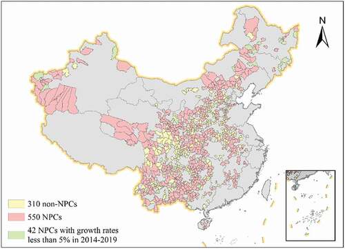
“Leaving no one behind” is a pledge of the United Nation’s Sustainable Development Goals (United Nations, 2015). Poverty alleviation has been a common goal and a major challenge of humanity (Bapna, 2012; Tollefson, 2015). In China, millions have been lifted out of poverty in recent decades, greatly contributing to global poverty alleviation (United Nations, 2015; Zhang, Xu, Sun, & Elahi, 2018; Zhou, Guo, Liu, Wu, & Li, 2018). Yet, more than 70 million people in China still lived below the extreme poverty line by 2015 (Xue & Weng, 2017) with several regions returning to poverty (Zhou et al., 2018). In 2014, China implemented an unprecedentedly ambitious “targeted poverty alleviation” (TPA) policy to combat poverty (Ge, Yuan, Hu, Ren, & Wu, 2017; Liu, Liu, & Zhou, 2017). Three basic policy instruments were emphasized by the government, including goal programming, financing support and infrastructure construction (Zhang et al., 2018). The most challenging target of TPA is 592 national poverty-stricken counties (NPCs) identified by the Poverty Relief Office of the State Council of China in 2012 (Figure 1). To date, however, it remains unknown about the actual successfulness of the TPA policy, including the spatial distribution of poverty alleviation across space and time. Such knowledge is crucial as China is facing the challenge of achieving sustainability under growing population, resource scarcity and large development inequalities across counties (Westmore et al., 2018; Xu et al., 2020; Zhang et al., 2018).

Figure 1. Spatial distribution of NPCs and non-NPCs

A major barrier to assess the successfulness of the TPA policy is lack of timely, reliable socioeconomic data. Intensive socioeconomic household surveys and census are costly and time consuming, making timely updates of poverty virtually impossible (Pokhriyal & Jacques, 2017). In fact, the survey and census data are not available for most counties in 2018 and all counties in 2019. Furthermore, the survey data in several regions of China remain unreliable (Lin, 2018; Wang & Zheng, 2018). Liaoning Province initially proposed the existence of GDP fraud, and Inner Mongolia also tried to obtain new subsidies from the central finance by admitting the financial data fraud. However, there are no NPCs in Liaoning Province and a few NPCs in the Inner Mongolia Autonomous Region, which have no substantial impact on the final results of the experiment.

Aiming at the difficulty of collecting data in the process of precise poverty alleviation, high cost and inconsistent statistics, the night light data and daytime remote sensing images are introduced. Based on the deep learning model, the poverty index prediction system is constructed. As a new learning mode in the field of machine learning, deep learning mainly uses convolution neural network as the carrier to construct an intelligent and efficient learning model, so as to solve the difficult problems in the field of natural science which depend on human brain. Sun, Di, and Sun et al. (2020) proposed a deep learning method for the Contiguous United States (CONUS) time-series (2012–2015) of GDP estimation at the county level. The model is developed by combining the NTL data from the visible infrared imaging radiometer suite day/night band and the MODIS land cover data. Sun et al. (2020) have studied all the counties in 5 developing countries, and we mainly carry out regression related indicators for NPCs in China, and the conclusions are more targeted. The results not only include the verification of correlation, but also analyze and evaluate the prediction results.

In this study, we propose a novel, independent approach combining satellite observations and deep learning to assess the successfulness of the TPA. We address four main questions. First, how is the reliability of our method for predicting economic growth? Second, how has economic development in the NPCs before/after the implementation of the TPA, especially at the county level? Third, how has economic development varied across the NPCs in different provinces over time? Fourth, how have differences in economic development between the NPCs and their neighboring non-NPCs evolved over time?

To answer these questions, we combine deep learning with multiple satellite datasets to estimate county-level economic development from 2008 to 2019 and assess the effect of the TPA policy for the 592 NPCs at country, provincial and county levels. As detailed in Methods, datasets used include remote sensing images (nighttime light data, Google Earth images, Sentinel-1, Sentinel-2 and Landsat 8 images), leaf area index (LAI) data, and county boundary data. Our deep learning framework is able to integrate disperse data with missing values from multiple sources to predict year- and county-specific population and GDP. Deep learning combining with large disparate data can effectively reduce the prediction bias caused by label noise and improve prediction performance. We train the deep learning model based on the survey data in 2008, 2011, 2013, 2015 and 2017, and validate the model using the survey data in 2009. We then use the model to estimate GDP and population of each NPC from 2008 through 2019, and calculate year- and county-specific per capita GDP and its annual growth rates. We compare per capita GDP results for the NPCs with those for neighbor non-NPCs and provincial average data to evaluate the successfulness of the TPA policy for these NPCs. Results from our timely, inexpensive method reveal an overall success of the policy so far as well as areas that need improved targeted support.

2. Methods

2.1. Data

2.1.1. Remote sensing data

Satellite remote sensing contributes substantially to our understanding of economic characteristics and social development. The potential of disparate satellite data to estimate socioeconomic factors has been proven (Pokhriyal & Jacques, 2017). Here, we use the following satellite data: nighttime light data, Google Earth images, Sentinel-1, Sentinel-2 and Landsat 8 images, and LAI data.

2.1.2. Nighttime light data

Nighttime light data is a useful spatial indicator for socioeconomic prediction, although it alone is difficult to differentiate economic activities in areas with populations living near or below the international poverty line (Dai, Hu, & Zhao, 2017; Gou & Yang, 2019; Huang, Wang, & Lu, 2019; Jean et al., 2016; Yeh et al., 2020). Here, we use two nighttime light datasets depending on the year and data availability. Over 2008–2012, we use the dataset from the US Air Force Defense Meteorological Satellite Program Operational Linescan System (DMSP/OLS), which has a spatial resolution of 2.7 km across an estimated 3,000 km of swath that covers the entire globe twice per day. Over 2013–2019, we use the average radiance composite images from the Visible Infrared Imaging Radiometer Suite Day/Night Band (VIIRS/DNB) produced by the Earth Observations Group at NOAA/NCEI, with a spatial resolution of 500 m. The temporal resolution of VIIRS/DNB data is annual for 2015–2016 and monthly for 2013–2014 and 2017–2019. We average the monthly data to obtain annual data for 2013–2014 and 2017–2019. We use the nighttime light data in 2015 as a mask to filter temporary lights and background (non-light) values.

To eliminate the inconsistency between DMSP/OLS and VIIRS/DNB data, we use the automatic invariant pixel method (Huang et al., 2019) to perform inter-sensor correction, continuity correction, and oversaturation correction on the DMSP/OLS night light images. Then, the VIIRS/DNB images with temporal overlap (2013) with DMSP/OLS are selected as a reference to calibrate all DMSP/OLS images at the VIIRS/DNB radiation level.

2.1.3. Optical images

The optical remote sensing images include Google Earth History images, Landsat 8 images and Sentinel-2 images to cover all years from 2008 through 2019. Google Earth History images include yearly data from 2008 through 2016, and are collected using the Google Static Maps API. We divide the Google Earth satellite images of each county into small tiles with 640 × 640 pixels; the size of each pixel is 17 m. All the images with blank regions occupying more than 50% of the area are excluded.

Since the Google Earth images do not cover the years of 2017–2019, we use Landsat 8 and Sentinel-2 images for 2017–2019 as supplements. Landsat 8 is equipped with an Operational Land Imager (OLI) that provides seasonal coverage of the global landmass at a spatial resolution of 30 meters (visible, NIR, SWIR). The Sentinel-2 satellite is equipped with an opto-electronic multispectral sensor for surveying with a resolution of 10 m in the visible light band. We collect yearly data over 2017–2019 from both Landsat 8 and Sentinel-2, and perform pixel cropping as done for the Google Earth images.

2.1.4. Sentinel-1 images

The Sentinel-1 satellite utilizes a C-band synthetic-aperture radar (SAR) instrument to acquire imagery regardless of weather and light conditions. Sentinel-1 images with a spatial resolution of 10 m record the backscattering coefficient of geographic scenes. Yearly data are available for 2015–2016, which are used here to identify roads and buildings, on the basis that these objects are brighter than others in the SAR images.

2.1.5. LAI product

We use the LAI product released by Beijing Normal University (Xiao et al., 2016), which is retrieved based on the MODIS (Moderate Resolution Imaging Spectroradiometer) and the Long-Term Data Record AVHRR (Advanced Very High Resolution Radiometer). We use data available in 2008–2019 in a sinusoidal projection at a spatial resolution of 1 km and a temporal resolution of 8 days. We combine the 8-day data to produce yearly data.

2.1.6. Combination of satellite data

We use the nighttime light intensities as the ground truth to label other satellite images. We use the optical images (from Google Earth, Landsat 8 and Sentinel-2), SAR images (from Sentinel-1) and LAI data to train and validate the deep learning model. In the Data Fusion module of the deep learning model, features of the optical images, SAR images and LAI data are extracted separately, and then the extracted features are transformed into the same feature space. Subsequently, a regression and a classification of the transformed features are done, using features from the nighttime light intensities as reference. Finally, the fused features are formed into a feature vector for the GDP and population prediction.

2.1.7. Economic and population survey data

We collect the county-level GDP and population survey data from 2008 through 2017 for 592 NPCs from the Economic Statistical Yearbook of their provinces. The county-level survey data are sparse for 2018 and have not been released for 2019.

For provincial and national-level analyses, the provincial average and national average per capita GDP data are taken from the China Statistical Yearbook.

2.2. Deep learning framework

We present a deep learning model to estimate yearly GDP and population of each county using the above disparate data sources. For the deep learning model, we use the satellite images, GDP and population of all NPCs in China in 2008 and 2009 as training data, and the dataset of all NPCs in 2017 as validation data. The trained model is then employed to predict GDP and population of other years.

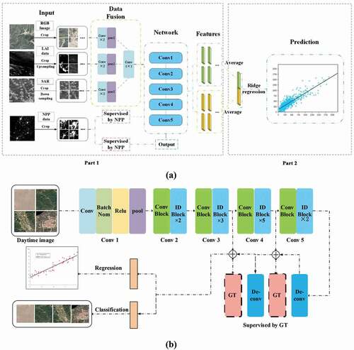
Figure 2(a) shows the framework of the deep learning model. Our model consists of two parts. The first part is an attention-driven deep learning network, which extracts feature vectors from the remote sensing images. We employ an adaptive layer (data fusion) prior to the network, and re-train the underlying network to make the adaptive layer keep the important information from the multi-source data. Because of the addition of the data fusion module, our network can accept images with any number of channels as input. This design allows easy addition of other data to improve the final prediction accuracy. The second part uses ridge regression to predict the economic indicators from the feature vector. We concatenate the features learned by different tasks as the input to the Ridge Regression model.

Figure 2. (a) Framework of our deep learning model; (b) Structure of our deep neural network

2.2.1. Data fusion

The versatile deep neural network uses three-channel RGB imagery as input. For our problem, however, using only RGB image loses a lot of extra information, and it is difficult for the network to learn features. In order to make full use of remote sensing images generated by different sensors, we design a Data Fusion module to automatically learn the features of different images through a convolutional network. We input the satellite images of the same area to the Data Fusion module. In this module, two convolutional layer and max pooling layer are applied to each data. Then, the 1 × 1 convolution layer fuse features extracted from different data and reduce the number of channels. The rest of improved ResNet50 layers are applied to the merged branch.

2.2.2. Extracting features from satellite images

Figure 2(b) shows the attention-driven deep learning framework. In the framework, we improve the network structure of ResNet50 (He, Zhang, Ren, & Sun, 2016) to better extract economy related features. The improved ResNet50 contains 49 convolution layers, uses stride = 2 for down-sampling and replaces the fully connected layer with a global average pool layer. The convolutional layer extracts features from the previous layer through the learned convolution kernel, which can produce different-level features such as the low-level features from the first layers and high-level features from the last layers. In the top layers of the improved ResNet50, the network mainly learns the features such as corners and edges. In the last layers, the feature representation of corners and edges fuses to the high-level feature like roads, rivers, villages, or towns. However, the features are not enough to represent the characteristics of different objects related to economic development. We introduce the attention model and multi-loss to focus on learning the features of the interested objects. The attention model integrates the spatial attention mechanism and channel-wise attention mechanism. The attention model guides the framework to pay more attention to the areas related to human activities by the supervision of the nighttime light. The multi-loss consists of the classification term and regression term. The classification term is used to classify the images into different light intensity categories. The regression term is designed to estimate the night light intensity value from the input satellite images.

2.2.3. Spatial and channel-wise attention

Attention is the means of allocating available computing resources to the most useful components of a signal (Hu, Shen, & Sun, 2018). Spatial attention drives the deep learning model to focus more on the interested regions, which helps to generate representative features. For the economic assessment, we use the area on the night light image whose intensity value is greater than zero as our attention region. We up-sample the feature maps by two deconvolution layers behind the improved ResNet50. The first deconvolution layer up-samples the feature map to 40 × 40 × 512 with the kernels size of 3 × 3 × 512. To make use of the shallow features and deep features, the output feature map of Conv 4 of ResNet50 is combined with the output of the first deconvolution layer. Then the convolution layer convolutes the output of the deconvolution layers to 40 × 40 × 1. We create a binary image as the ground truth if the value of the light intensity is larger than 0. The output features are supervised by the binary image to highlight the interested regions. The second layer of deconvolution and subsequent operations are the same as the previous layer. The spatial attention map f_att is generated as follows:

(2) $f_{att}\left(x,y\right)=f_d\left(x,y\right)\times f_c\left(x,y\right)$(2)

where $f_d\in R^{W\times H\times C}$ denotes the output feature map of the second deconvolution layer, $f_c\in R^{W\times H\times 1}$ denotes the output of the convolution layer in the attention module, and$(\mathrm{x},y)$is the spatial location in the map.

As ResNet50 deals with the convolutional features, it treats all channels equally. However, the generated features of different channels in the CNN have different semantics. It is necessary to introduce channel-wise attention to find more critical feature channels.

We integrate the Squeeze-and-Excitation block into the ResNet50. In the block, the squeeze operation is a global average pooling layer, which pools the H × W × C feature maps U to a vector of 1 × 1 × C. Then, the output vector goes through the excitation operation, and two layers of the fully connected layers, and then uses the sigmoid function to normalize the value to the range of [0, 1] as the weight scale factor for each channel. Finally, U multiplying this value is mapped to the C channels as the input data of the next level. This structure is to strengthen the key channels and weaken the unimportant channels by controlling the scale, so that the extracted features are more directional. The whole process can be described as the follows.

In the squeeze operation, we write the outputs of $F_{sq}$ as $Z=[z_1,z_2,\dots ,z_c],$

(3) $z_{\mathrm{c}}=F_{sq}(u_c)=\frac{1}{H\times W}\sum _{i=1}^H\sum _{j=1}^W{u}_c(i,j).$(3)

In the excitation operation,

(4) $s=F_{ex}\left(z,W\right)=\sigma \left(W_2\delta \left(W_{1}z\right)\right)$(4)

where δ denotes the ReLU function, $W_{\mathbf{1}}\in {\mathrm{R}}^{\frac{c}{r}\times c}$, and $W_2\in {{\mathrm{R}}^{c\times }}^{\frac{c}{r}}$are parameters of two fully connected layers. r is a reduction ratio which reduces the output dimension of the first fully connected layer, and then restores to the original number on the second fully connected layer.

2.2.4. Multi-loss

The ground-truth class labels of each remote sensing image are determined according to the total nighttime light intensities. The classifier is a 2-way fully-connected layer behind the spatial attention term with 1,024 neurons and a softmax activation layer. In the classification term, the cross-entropy loss is employed, which is formulated as:

(5) $L_c=-\frac{1}{n}\sum _{i=1}^n{y}_{ij}log{\hat{p}}_{ij}+\left(1-{\mathrm{y}}_{\mathrm{i}\mathrm{j}}\right)log\left(1-{\hat{\mathrm{p}}}_{\mathrm{i}\mathrm{j}}\right)$(5)

where y_ij∈[0, 1] denotes the j-th dimension of the ground-truth class label vector for the training image i, ${\hat{p}}_{ij}$ is the output of the softmax layer, and n is the batch size.

For the regression term, the mean absolute error (MAE) loss is employed to measure the predicted nighttime light intensities. The MAE loss was formulated as:

(6) $L_r=\frac{1}{n}\sum _{i=1}^n\left|b_i-{\hat{b}}_i\right|$(6)

where ${\hat{b}}_i$ is the output of the regression layer, and n is the batch size.

The classification branch and the regression branch each generate a 1,024-dimensional feature vector, and we concatenate the two vectors together as the input to the ridge regression.

2.2.5. Ridge regression

The deep neural network produces a 2,048-dimensional feature vector by a global average pooling layer from each satellite image. All images feature vectors of one county are averaged into a single vector. We separately use the normalized GDP and population along with the corresponding image vector to train the regularized ridge regression model. Ridge regression is a linear regression model, which imposes a square penalty on the magnitude of linear coefficients. When the correlation between our features is high, ridge regression is suitable. In our method, the feature has 2,048 dimensions, so regularization is used to eliminate over-fitting.

2.2.6. Training and testing algorithm

We train the attention-driven network model on an Ubuntu 16.04 computer with Intel i7-6850 K CPU using two NVIDIA GTX 1080Ti 11Gb GPUs. The network is trained using stochastic gradient descent with 48 images as a mini-batch and a learning rate of 0.01. We use a weight decay of 10^–4 and a momentum of 0.9. The weights of all filters are initialized with the pre-trained weight on the ImageNet dataset. Then, it is fine-tuned on our dataset with the Keras 2.0 platform. A total of about 42,000 images are selected as the training samples, and 24,610 images are used as the validation samples.

2.3. Deep learning based estimate

The deep learning approach is trained and validated based on data for the NPCs and non-NPCs together. The non-NPCs are more affluent counties not assigned as NPCs at present. We first sort the 592 NPCs in the descending order of per capita GDP in 2013, and then divide the NPCs into 16 quantile ranges. There are 37 NPCs in each quantile range. We then select 310 non-NPCs adjacent to the NPCs in these quantile ranges, with each quantile range containing 8–32 non-NPCs (Supplementary Table 1). The per capita GDP of each selected non-NPC is close to its respective adjacent NPC. Specifically, the difference in per capita GDP in 2013 between any non-NPC and its paired NPC is below 1,400 Yuan in each of the first 14 quantile ranges and is below 2700 Yuan in the 16th (i.e. richest) quantile range.

According to Benford’s law, Gou and Yang (2019) got 133 data units of department expenditure final accounts data fitting degree, and the comprehensive rating was excellent or good, the excellent and good rate was 100%. The quality of expenditure final accounts data was excellent, and there was no man-made data manipulation or systematic error. We use Benford’s law (Judge & Schechter, 2009) to assess the official county-level data in 2008–2017 obtained from Province Statistical Yearbook of China (Methods, Supplementary Table 2). We find the data in 2008, 2009, 2011, 2013, 2015 and 2017 to be more reliable than those in other years. Thus we choose the data in 2008, 2011, 2013, 2015 and 2017 to train our deep learning based framework, and use the data in 2009 to validate the framework.

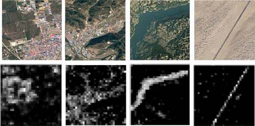
The deep learning approach is illustrated in Figure 2. It relies on spatial features contained in remote sensing images to estimate population and GDP of each county. To evaluate whether the learned feature representation by our framework can distinguish different object categories from remote sensing images, we map the high-dimensional learned feature to a 2-D space. The final feature layer is obtained by averaging each feature layer in the deep learning model. Figure 3 shows an example of the extracted features of different categories in the NPCs. It is observed that the deep learning model is able to recognize semantically meaningful features from the remote sensing images with cluttered background.

Figure 3. Visualization of the extracted features. The first row illustrates four object categories in remote sensing images: farmland, town, river and road. The second row shows the features of the four objects learned by our method from the corresponding images in the first row

3. Results

3.1. Estimation of affluence

Based on the deep learning predicted GDP and population of each county from 2008 to 2019, we calculate the respective per capita GDP and its annual growth rate (AGR-pcGDP) for 2009–2019; here, the AGR-pcGDP for a given year represents the growth from its previous year to that year. The AGR-pcGDPs of the 592 NPCs and 310 non-NPCs before (2009–2013) and after (2014–2019) the implementation of TPA are analyzed at three spatial levels, i.e. country-level, provincial-level and county-level. Unless stated otherwise, all results presented for the NPCs and non-NPCs are predicted from our deep learning model.

3.2. Assessment of GDP and pcGDP

Supplementary Table 3 shows that the coefficient of determination (R²) and normalized mean bias (NMB) for the predicted GDP relative to survey data across the 592 NPCs on a yearly basis. Although the NMB is small in each year, the R² varies from 0.78 to 0.93 over 2008–2017. The respective coefficients of determination are 0.76–0.93 for population and 0.61–0.83 for per capita GDP. These reflect the large scatter in data consistency across the individual NPCs, as shown in the scatterplots in Supplementary Figure 1 for per capita GDP. Therefore precisely estimating the AGR-pcGDP of a single county is difficult. However, when results are averaged in any but the first of the 16 quantile ranges, we find high correlations across the years between the predicted and surveyed per capita GDP data for the NPCs (R² ≥ 0.92) and for their respective non-NPCs (R² ≥ 0.94) (Supplementary Table 1). This provides a basis for our quantile-based analysis. The correlation is lower (R² = 0.72) for the NPCs in the first quantile range (i.e. the poorest), whose AGR-pcGDP is thus not analyzed in the following.

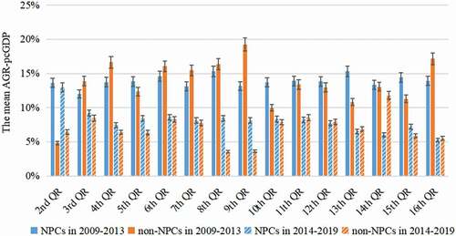
Figure 4 shows a general reduction in the average AGR-pcGDP of NPCs in each quantile range from before (2009–2013) to after (2014–2019) the implementation of TPA. This reflects the influence of global financial crisis and the slowdown in Chinese economic growth. After the TPA, the AGR-pcGDPs of NPCs in most quantile ranges (QR, from 2^nd to 10^th and the 15^th) are higher those of non-NPCs by 0.3%-6.5%, whereas the AGR-pcGDPs of NPCs in the 11^th, 12^th, 13^th, 14^th and 16^th quantile ranges are lower than those of non-NPCs by 0.2%-5.8%. Overall, the NPCs have experienced sustained high growth rates (5.3%-13.0% across the quantile ranges) after the implementation of the TPA. The poorer NPCs in the first 10 quantile ranges have grown faster than the richer NPCs in the last 5 quantile ranges after the TPA, likely indicating a greater success of the TPA in supporting the poorer NPCs.

Figure 4. Average AGR-pcGDP of the NPCs in each quantile range and their respective non-NPCs. Error bars indicate 1 standard deviation across the counties

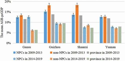
The 592 NPCs are located in 21 provinces (Figure 4). A disproportionally large number of NPCs (at least 50) are located in each of Gansu, Guizhou, Shaanxi and Yunnan provinces in western China. Compared to more affluent regions, these four provinces have relatively inconvenient transportation, weak infrastructure and limited socioeconomic development, and have the lowest industrialization level and the highest poverty rate in China. We thus focus on the NPCs in these four less developed provinces to further assess the economic development of the NPCs.

For each province, we compute the correlations between the predicted provincial average (from all NPCs) annual per capita GDP and the respective survey data. Supplementary Table 4 shows high correlations (R² ≥ 0.96) between the prediction and survey data of the NPCs in the four provinces. For comparison, we also select the non-NPCs in each province from the aforementioned non-NPC list, including 8 in Gansu, 6 in Guizhou, 18 in Shaanxi, and 21 in Yunnan, with a total of 45. Supplementary Table 4 shows high correlations (R² ≥ 0.92) between the prediction and survey data for the 45 non-NPCs.

Figure 5 shows that before the TPA, the average AGR-pcGDP of the non-NPCs in each of the four provinces is higher than that of their NPCs by 0.1%–4.7%. After the TPA, the average AGR-pcGDPs of the NPCs in Gansu, Guizhou and Yunnan provinces are higher than those of the corresponding non-NPCs by 6.4%, 0.4% and 0.6%, respectively. In Shaanxi, the difference in AGR-pcGDPs between the NPCs and non-NPCs is reduced from 4.7% before the TPA to 1.1% after the TPA. The growth rates of the NPCs are much larger than the provincial average obtained from the Statistical Yearbook in Gansu and comparable to the provincial average in Guizhou, Shaanxi and Yunnan. Further targeted support is needed in the latter three provinces to fasten the growth of their NPCs.

Figure 5. Average AGR-pcGDPs for the NPCs and non-NPCs in the four provinces. Error bars indicate 1 standard deviation across the counties. The provincial growth rates data are obtained directly from the China Statistical Yearbook for comparison

We compare the average AGR-pcGDP of the 592 NPCs with that of the 310 respective non-NPCs. We also examine the growth rate of the national average per capita GDP taken from the China Statistical Yearbooks. Our predicted per capita GDP averaged over the 592 NPCs and over the 310 non-NPCs are highly consistent with the respective survey data, with the coefficients of determination exceeding 0.99.

Figure 6 compares the average AGR-pcGDP of the 592 NPCs, of the 310 non-NPCs, and of the whole country. For each case, the AGR-pcGDP exceeds 5.0% in most years from 2009 to 2019. The average AGR-pcGDP of the 592 NPCs fluctuates greatly between 18.4%±2.2% (mean ± standard deviation; in 2010) and 6.1%±0.7% (in 2016). Over 2014–2019 (after the TPA), the average AGR-pcGDPs of NPCs are generally lower than in previous years because of the aforementioned slowdown of Chinese economic growth. Nevertheless, the average AGR-pcGDP of NPCs is higher than the whole country for most years, indicating that China’s poorest counties have grown at faster rates than the national average during the past decade.

Figure 6. AGR-pcGDP of 592 NPCs, 310 adjacent non-NPCs, and the whole country over 2009–2019. Error bars indicate 1 standard deviation across the counties. The national data are taken directly from the Statistical Yearbooks

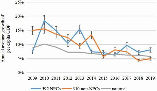
Compared to the 310 non-NPCs, the 592 NPCs as a whole have grown slower in 2014 and 2016 but faster in 2015, 2017, 2018 and 2019. Averaged over 2014–2019, the mean AGR-pcGDP of all NPCs (7.6%±0.4%) is higher than that for the 310 non-NPCs (7.3%±0.4%), and for the whole country (6.3%) (Supplementary Figure 2). These results indicate that the TPA has an overall targeted, positive effect on the growth of NPCs.

3.3. Room for policy improvement

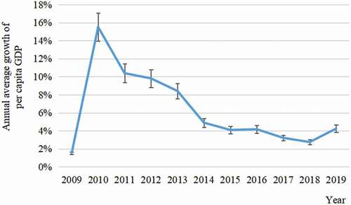
Not all NPCs have experienced sustained high growth rates, based on our estimate. There were 42 NPCs (Figure 1) whose average AGR-pcGDP has declined over the years to values less than 5.0% (Figure 7), much lower than the mean AGR-pcGDP of all NPCs. Most of these NPCs are in areas with inconvenient transportation and poor natural conditions, or rely heavily on resource-consuming enterprises that are affected by continuously strengthened environmental protection policies. More targeted support, financially and/or technologically, should be given to these NPCs.

Figure 7. Variations in the average AGR-pcGDP of the 42 NPCs with weak growth. Error bars indicate 1 standard deviation across the counties

In 2019, the predicted average per capita GDP of 592 NPCs is 23,750 Yuan (3,358.9 US Dollar), which is still much lower than that of the whole country (70,892 Yuan). The difference between predicted per capita GDP of NPCs and the provincial average in 2019 is also large in the four provinces with the largest number of NPCs: 17,039 versus 32,995 Yuan in Gansu, 20,715 versus 46,433 Yuan in Guizhou, 29,837 versus 66,649 Yuan in Shaanxi, and 18,802 versus 47,944 Yuan in Yunnan. These results suggest a long way for the NPCs to go to reach the average affluence level of the nation/province.

4. Discussion

This study can acquire the regression results of NPCs through the combination of deep learning network and remote sensing image only. The high temporal resolution of remote sensing images makes this method can obtain information quickly and timely. Our study has two limitations. Due to a lack of temporal labels for the daytime imagery (i.e. the exact date of each image is unknown), the prediction power of the deep learning model could be decreased. In recent years, more people in poor regions in China moved to the developed regions for work. Our study is difficult to deduce the effect of internal migration on income of the family in the NPCs. Remittance is an important income source for the poor regions, and such quantity is not captured. This is the first study to evaluate the long-term impact of China’s TPA policy on poverty mitigation at the county level. Our results based on national, provincial and county-level analyses suggest that since 2014, the affluence of NPCs measured by per capita GDP has on average grown at a faster rate than those of adjacent non-NPCs. This suggests an overall success of the TPA policy so far, and by 2020, all NPCs were out of poverty. However, the growth rates of many NPCs have decline to values below 5% in recent years, and the predicted average affluence of the NPCs in 2019 is still much lower than the levels of the nation and respective provinces. Continuous, sufficient targeted support to the NPCs is still needed to enhance their economic performance and social welfare.

Note that people in poor regions of China can move to developed regions for work, but our model cannot fully capture the effect of migration on income. Nonetheless, the increased income of migrants is often sent back to their hometowns and spent on housing and other aspects that affect land use, land cover and/or nighttime light. Such an indirect effect is captured by the satellite data and our model framework.

Our results can be affected by the quality of county-level survey data. We investigate this issue based on available information. The local governments in Inner Mongolia have admitted their published survey data in 2014 to be un-authentically high. Through strict supervisions, their survey data quality has been improved since 2017. The correlations between the survey data and our predicted results in 2014, 2017 and 2018 are 0.64, 0.88 and 0.72, respectively. The higher correlations in 2017 and 2018 reflect the surface data improvement. This is consistency with the results of survey data quality assessment based on Benford’s law (Supplementary Table 5).

This study demonstrates the capability of deep learning combined with publically available timely data sources in estimating socioeconomic development. The estimates are close to the official survey data. Our approach is not able to precisely predict GDP and population of each single county. However, combining results from multiple counties greatly reduces the influence of random errors and leads to satisfactory prediction of GDP, population and affluence, at the expense of spatial resolution reduction. Our inexpensive, convenient and reliable model framework for socioeconomic prediction complements the official data obtained through time consuming and resource expensive surveys. In particular, our framework can be applied to areas difficult to reach by census takers and to times with survey data unavailable.

Data availability statement

The Per capita GDP results and growth rates at different levels are available at https: 10.6084/m9.figshare.15052545 and https://www.doi.org/10.11922/sciencedb.j00076.00089.

Disclosure statement

No potential conflict of interest was reported by the author(s).

Supplementary material

Supplemental data for this article can be accessed here.

Additional information

Funding

This work was supported by the National Natural Science Foundation of China under Grant No. 41925006.

Notes on contributors

Yanxiao Jiang

Yanxiao Jiang is currently working toward the master's degree in the Faculty of Geographical Science, Beijing Normal University, China. Her research interests include machine learning, remote sensing imagery processing and application.

Liqiang Zhang

Liqiang Zhang received the Ph.D. degree in geoinformatics in 2004 from the Institute of Remote Sensing Applications, Chinese Academy of Science. He is currently a Professor with the Faculty of Geographical Science, Beijing Normal University, China. His research interests include remote sensing image processing, 3D urban reconstruction, and spatial object recognition.

Yang Li

Yang Li is currently working toward the master’s degree in the Faculty of Geographical Science, Beijing Normal University, China. His research interests include deep learning and remote sensing image processing.

Jintai Lin

Jintai Lin received the Ph.D. degree from the University of Illinois at Urbana Champaign, in 2008. He is currently an associate Professor with the department of atmospheric and Marine Sciences, School of physics, Peking University, China. His research interests include atmospheric chemistry, satellite remote sensing, and global air pollution.

Suhong Liu

Suhong Liu received the B.S. degree in computer science from Southwest Jiaotong University, China, in 1988, the M.S. degree in geophysical well-logging from Jianghan Petroleum University, China, in 1991, and the Ph.D. degree in cartography and remote sensing from the Institute of Remote Sensing Applications, Chinese Academy of Sciences, in 1999. She is currently a Professor with the Faculty of Geographical Science, Beijing Normal University. Her research interests include spatio-temporal analysis of remotely sensed data and retrieval of land biophysical parameters from satellite data.

References

- Bapna, M. (2012). World poverty: Sustainability is key to development goals. Nature, 489(7416), 367.
- Dai, Z., Hu, Y., & Zhao, G. (2017). The suitability of different nighttime light data for GDP estimation at different spatial scales and regional levels. Sustainability, 9(2), 305.
- Ge, Y., Yuan, Y., Hu, S., Ren, Z., & Wu, Y. (2017). Space-time variability analysis of poverty alleviation performance in China’s poverty-stricken areas. Spatial Statistics, 21, 460–474.
- Gou, X., & Yang, J. (2019). Application of Benford’s law in data quality evaluation of department final accounts. Public Finance Research, (2), 26–42.
- He, K., Zhang, X., Ren, S., & Sun, J. (2016). Deep residual learning for image recognition. IEEE Conference on Computer Vision and Pattern Recognition, Las Vegas, NV, USA. doi: https://doi.org/10.1109/CVPR.2016.90
- Hu, J., Shen, L., & Sun, G. (2018). Squeeze-and-Excitation Networks. IEEE Conference on Computer Vision and Pattern Recognition, Salt Lake City, UT, USA, 7132–7141. doi: https://doi.org/10.1109/TPAMI.2019.2913372
- Huang, X., Wang, C., & Lu, J. (2019). Understanding the spatiotemporal development of human settlement in hurricane-prone areas on the US Atlantic and Gulf coasts using nighttime remote sensing. Natural Hazards and Earth System Sciences, 19(10), 2141–2155.
- Jean, N., Burke, M., Xie, M., Davis, W. M., Lobell, D. B., & Ermon, S. (2016). Combining satellite imagery and machine learning to predict poverty. Science, 353(6301), 790–794.
- Judge, G., & Schechter, L. (2009). Detecting problems in survey data using Benford’s Law. Journal of Human Resources, 44(1), 1–24.
- Lin, W. (2018). Discussion on subtle central-local economic relations and their reshaping and adjustment from the phenomenon of data falsification. China Market, 973(18), 28–30.
- Liu, Y., Liu, J., & Zhou, Y. (2017). Spatio-temporal patterns of rural poverty in China and targeted poverty alleviation strategies. Journal of Rural Studies, 52, 66–75.
- Pokhriyal, N., & Jacques, D. C. (2017). Combining disparate data sources for improved poverty prediction and mapping. Proceedings of the National Academy of Sciences, 2017, 114(46): E9783-E9792.
- Sun, J., Di, L., Sun, Z., Wang, J., Wu, Y. (2020). Estimation of GDP using deep learning with NPP-VIIRS imagery and land cover data at the county-level in CONUS. IEEE Journal of Selected Topics in Applied Earth Observations and Remote Sensing, 99, 1–1. doi:https://doi.org/10.1109/JSTARS.2020.2983331
- Tollefson, J. (2015). Can randomized trials eliminate global poverty? Nature, 524(7564), 15–153.
- United Nations. (2015). The Millennium Development Goals Report 2015. New York.
- Wang, H., & Zheng, K. Y. (2018). Analysis for recent adjustment of statistical data in some provinces. China Market, (36), 10–12. doi:https://doi.org/10.1080/10130950.2009.9676265
- Westmore, B. (2018). Do government transfers reduce poverty in China? Micro evidence from five regions. China Economic Review, 51, 59–69.
- Xiao, Z., Liang, S., Wang, J., Xiang, Y., Zhao, X., & Song, J. (2016). Long-time-series global land surface satellite leaf area index product derived from MODIS and AVHRR surface reflectance. IEEE Transactions on Geoscience and Remote Sensing, 54(9), 5301–5318.
- Xu, Z., Chau, S. N., Chen, X., Zhang, J., Li, Y., Dietz, T., … Liu, J. (2020). Assessing progress towards sustainable development over space and time. Nature, 577(7788), 74–78.
- Xue, L., & Weng, L. (2017). The policy opportunities and challenges in China’s implementation of 2030 sustainable development goals. China Soft Science, 1, 1–12.
- Yeh, C., Perez, A., Driscoll, A., Azzari, G., Tang, Z., Lobell, D., … Burke, M. (2020). Using publicly available satellite imagery and deep learning to understand economic well-being in Africa. Nature Communications, 11(1), 2583.
- Zhang, H., Xu, Z., Sun, C., & Elahi, E. (2018). Targeted poverty alleviation using photovoltaic power: Review of Chinese policies. Energy Policy, 120, 550–558.
- Zhou, Y., Guo, Y., Liu, Y., Wu, W., & Li, Y. (2018). Targeted poverty alleviation and land policy innovation: Some practice and policy implications from China. Land Use Policy, 74, 53–65.