A lake ice phenology dataset for the Northern Hemisphere based on passive microwave remote sensing

ABSTRACT

Lake ice phenology (LIP) is an essential indicator of climate change and helps with understanding of the regional characteristics of climate change impacts. Ground observation records and remote sensing retrieval products of lake ice phenology are abundant for Europe, North America, and the Tibetan Plateau, but there is a lack of data for inner Eurasia. In this work, enhanced-resolution passive microwave satellite data (PMW) were used to investigate the Northern Hemisphere Lake Ice Phenology (PMW LIP). The Freeze Onset (FO), Complete Ice Cover (CIC), Melt Onset (MO), and Complete Ice Free (CIF) dates were derived for 753 lakes, including 409 lakes for which ice phenology retrievals were available for the period 1978 to 2020 and 344 lakes for which these were available for 2002 to 2020. Verification of the PMW LIP using ground records gave correlation coefficients of 0.93 and 0.84 for CIC and CIF, respectively, and the corresponding values of the RMSE were 11.84 and 10.07 days. The lake ice phenology in this dataset was significantly correlated (P<0.001) with that obtained from Moderate Resolution Imaging Spectroradiometer (MODIS) data – the average correlation coefficient was 0.90 and the average RMSE was 7.87 days. The minimum RMSE was 4.39 days for CIF. The PMW is not affected by the weather or the amount of sunlight and thus provides more reliable data about the freezing and thawing process information than MODIS observations. The PMW LIP dataset provides the basic freeze–thaw data that is required for research into lake ice and the impact of climate change in the cold regions of the Northern Hemisphere. The dataset is available at http://www.doi.org/10.11922/sciencedb.j00076.00081.

KEYWORDS:

• Lake ice phenology dataset
• Northern Hemisphere
• passive microwave remote sensing

1. Introduction

Lake ice is one of the key Environmental Climate Variables (ECVs) in the Global Climate Observing System (GCOS) (National centers for environmental information [EB/OL], 2017). Lake ice thickness, extent and phenology, and the changes of these parameters are key factors in climate and regional ecological research. Every winter, more than 50 million lakes around the world freeze over (Filazzola, Blagrave, Imrit, & Sharma, 2020).

Lake ice phenology describes the seasonal cycle of lake freezing and thawing. Four main parameters are usually considered: these are the Freeze Onset (FO), Complete Ice Cover (CIC), Melt Onset (MO), and Complete Ice Free (CIF) dates (Duguay et al., 2006; Kang, Duguay, & Howell, 2011). Research on lake ice phenology has shown that there is a widespread trend toward later freezing, earlier break-up, and shorter ice-cover duration on the Tibetan Plateau (Cai et al., 2019; Kropácek, Maussion, Chen, Hoerz, & Hochschild, 2013; Ruan, Zhang, Xin, Qiu, & Sun, 2020), in the Pan-Arctic (Karetnikov, Leppäranta, & Montonen, 2017; Šmejkalová, Edwards, & Dash, 2016) and North America (Latifovic & Pouliot, 2007) and across the world as a whole (Magnuson et al., 2000; Su, Che, & Dai, 2021).These results are obtained both by inverting remote sensing observations (mostly for the period after 2000) and from ground observations (mainly before 2000). It has been demonstrated that lake ice phenology is correlated with the loss or gain of lake water and with lake surface temperature changes (Woolway et al., 2020; Zhang et al., 2020). According to relevant spatiotemporal data series, 14,800 lakes currently have intermittent ice cover in world; this is expected to increase to 35,300 lakes for an increase of 2°C in average global air temperature and to 230,400 for an 8°C increase (Sharma et al., 2019). Lake ice constitutes one of the most important stores of fresh water ice on the Earth’s surface (Lu et al., 2020; Sharma et al., 2020), and changes in lake ice phenology have a notable effect on the climate, environment, and social and economic activity (Leppäranta, 2015; Sharma et al., 2019; Woolway et al., 2020). Earlier melting of lake ice in spring will cause greenhouse gases stored in the lake to be released earlier, seriously affecting the ecological environment (Denfeld, Baulch, Giorgio, Hampton, & Karlsson, 2018).

To understand changes in lake ice phenology, continuous and sustainable observations made at large spatiotemporal scales are needed. Lake ice phenology records are mainly derived from ground observations and remote sensing data. Long term records are available for most ground stations. The Global Lake and River Ice Phenology Database (GLRIPD) released by the National Snow and Ice Data Center (NSIDC) includes the freezing and thawing dates of rivers and lakes in 12 countries: these data include ice-on and ice-off records for 631 lakes, with 249 of these records covering a period of 50 years and 66 covering a period of 100 years (Benson, Magnuson, & Sharma, 2000). The Canadian Lake Ice Database published by the Canadian Cryospheric Information Network (CCIN) contains the freezing and melting dates for 258 lake sites in Canada from 1822 to 1999 (Canadian Cryospheric Information Network, 2017). For some of these sites, records of the ice thickness and snow depth are also included. However, ground observations are limited by observers’ experience and the harsh location of the observation sites, the ground observations records only contain the ice phenology within the visual range of the observer. This is a problem for large lakes in particular. As satellite technology has improved, it has become possible to carry out continuous monitoring of lakes in regions with harsh environments, such as the Tibetan Plateau. About 40 years of satellite observations are now available, these provide long time-series of data that can be used for lake ice monitoring.

Passive microwave (PMW) sensors are well suited to the monitoring of the ice phenology of large lakes. PMW satellite data have a revisit cycle of 1–2 days at middle and low latitudes and of less than once a day in high latitudes (Qiu, Guo, et al., 2017; Wu, Duguay, & Xu, 2020). However, observations are hampered by the poor spatial resolution of the sensors (tens of kilometers). The freezing and thawing processes in small lakes occur quickly and satellite data with high spatial and temporal resolutions would be needed for monitoring them (Zhang & Pavelsky, 2019). The Moderate Resolution Imaging Spectroradiometer (MODIS) carries out daily observations at high spatial resolution. However, the optical remote sensing data acquired by MODIS cannot be used to obtain information about lake ice phenology in poor weather and light conditions. In contrast, PMW sensors are not affected by cloud, rain, or daylight conditions and can therefore provide temporally and spatially continuous information on the freezing and thawing of lakes. Recently, the freezing and thawing of 71 lakes in the Northern Hemisphere was assessed using enhanced-resolution PMW observations (Du, Kimball, Duguay, Kim, & Watts, 2017). In other studies, optical remote sensing data were used to assess the ice coverage of 308 lakes on the Tibetan Plateau (Qiu et al., 2019) and the freezing and thawing of more than 13,300 lakes in the Pan-Arctic region (Šmejkalová et al., 2016). Although many lakes in the Northern Hemisphere have been monitored, the number of lakes monitored in individual studies has been limited, especially in inner Eurasia. Also, the use of different data sources has led to errors in comparative analyses of lake ice phenology between various regions (Qiu, Massimo, et al., 2017; Guo, Li, & Qiu, 2020; Li et al., 2020).

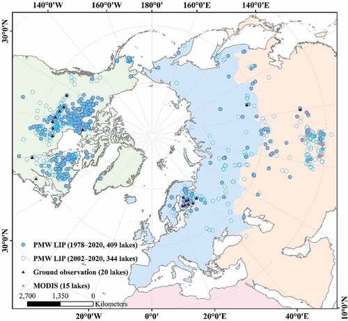
In order to obtain a long-term time-series of lake ice phenology, in this study, Ku-band (~ 19 GHz) horizontally polarized passive microwave data were used as the input, and lake brightness temperatures (Tb) were derived based on a nearest-neighbor algorithm. From the brightness temperatures, the FO, CIC, MO, and CIF dates were then obtained for 753 lakes in the Northern Hemisphere for the period 1978 to 2020 (Figure 1). The Northern Hemisphere Lake Ice Phenology (PMW LIP) dataset based on passive microwave data combined with ground observations (e.g. NSIDC and CCIN) and remote sensing products (e.g. lake ice extent products based on MODIS) provides a freeze–thaw dataset for more than 1,000 lakes in high-altitude and high-latitude regions.

Figure 1. The distribution of the 753 lakes in the Northern Hemisphere that were the subject of this study. The dark/light blue circles represent different types of data coverage and the dark/light red triangles represent the use of different verification data.

2. Data and methods

2.1. Data sources

Horizontally polarized 19-GHz PMW brightness temperature data acquired during descending orbits from 1978 to 2020 were obtained for use as the input to the ice phenology algorithm. The sources of the brightness temperature data consisted of Calibrated Passive Microwave Daily EASE-Grid 2.0 (CETB), Microwave Radiation Imager (MWRI), and Advanced Microwave Scanning Radiometer 2 (AMSR2) data. CETB data have a resolution of 6.25 km×6.25 km and cover the period from October 1978 to December 2019 (Brodzik, Long, Hardman, Paget, & Armstrong, 2016), and the spatial resolution of data was designed to be as good as possible while keeping the amount of noise low (Long, Brodzik, & Hardman, 2019). The dataset consists of data acquired by the Nimbus-7 Scanning Multichannel Microwave Radiometer (SMMR) (Gloersen & Barath, 1977) from October 1978 to August 1987, the Special Sensor Microwave Imager Sounder (SSM/I) (Hollinger, Peirce, & Poe, 1990) from September 1987 to December 2019, the Special Sensor Microwave Imager/Sounder (SSMIS) series of sensors from September 2005 to December 2019, and the Advanced Microwave Scanning Radiometer (AMSR-E) (Kawanishi et al., 2003) from June 2002 to November 2011.

After AMSR-E ceased operations on November 4, 2011, AMSR2 was successfully launched on May 18, 2012 onboard the sun-synchronous JAXA GCOM-W1 satellite. The missing data for the period November 2011 to May 2012 were supplemented by data acquired by the MWRI sensor carried by the Fengyun-3 series satellites (Yang et al., 2009, 2011). These data can be obtained from the Chinese National Satellite Meteorological Center (NSMC). The frequency, incidence angle, and orbital equatorial crossing time of MWRI, AMSR2, and AMSR-E are similar. The spatial resolution of AMSR2 is better than that of AMSR-E, and the AMSR2 L1 R data used in this study have a resolution of 22 km×14 km in the 18.7 GHz channel (Maeda et al., 2011). Table 1 shows the sensors, sources, and characteristics of the data used to generate the ice phenology dataset.

Table 1. Sources and characteristics of PMW data used in this study.

Period of coverage	Sensor	Frequency (GHz)	Spatial Resolution(km×km)	Source
Enhanced data				NSIDC (The Calibrated Passive Microwave Daily EASE-Grid 2.0 data, https://nsidc.org/data/NSIDC-0630/versions/1)
October 1978 to July 1987	SMMR	18.0	6.25 × 6.25 (enhanced resolution)
August 1987 to May 2002	SSM/I	19.35
June 2002 to July 2011	AMSR-E	18.7
L1 data
August 2011 to August 2012	MWRI	18.7	50 × 30	NSMC (http://data.nsmc.org.cn)
September 2012 to September 2020	AMSR2	18.7	22 × 14	JAXA (http://global.jaxa.jp/)

2.2. Processing of brightness temperature data

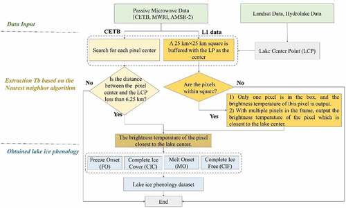
A system was developed to automatically obtain the position of the Lake Center Point (LCP) for each of the target lakes. This also enabled preprocessing of the PMW L1 data into a suitable format for use in the ice phenology algorithm and the data were also georeferenced. Two nearest neighbor algorithms were used to extract the daily brightness temperature from the data satellite data – the algorithm that was used depended on the data source. The extraction of the lake ice phenology was based on the difference between the emissivity of ice and water. For the enhanced PMW data, the pixel closest to the LCP and the brightness temperature of the pixel were directly collected. In the case of the L1 PMW data, a square was formed with the LCP as the center, and the brightness temperature of the pixel closest to the LCP was taken as the brightness temperature of the LCP. Finally, the lake ice phenology was derived from the long time-series of collocated brightness temperatures using a change-detection approach. As a result, the lake Freeze Onset (FO), Complete Ice Cover (CIC), Melt Onset (MO), and Complete Ice Free (CIF) dates were obtained for the 753 target lakes. A flow chart illustrating the ice phenology algorithm is shown in Figure 2, further details are explained in the following subsections.

Figure 2. The different components of the lake ice phenology algorithm that was developed in this study.

2.2.1. Identification of lake positions

Before the low-resolution passive microwave data were processed, a suitable set of lakes was first selected for study. To reduce the effect of mixed land pixels, lakes with areas of more than 40 km² were selected according to the areas given in the HydroLAKES database (Messager et al., 2016); the resolution of the CETB (6.25 km×6.25 km) was also considered when choosing this threshold. Lakes in regions that are tropical or subtropical according to the Köppen climate classification (Beck et al., 2018) and that do not freeze were also excluded. The coordinates of the LCPs were then obtained using HydroLAKES and Google Earth. Many lakes have irregular shapes, and the automatically extracted LCP maybe appear in narrow water, making the brightness temperature data obtained contain more land pixels. Therefore, we selected the central coordinates of the large water areas as the LCP. Finally, 3,237 sets of LCP coordinates were obtained.

2.2.2. Extraction of lake brightness temperature using the nearest neighbor algorithm

1) Brightness temperature extraction from CETB

CETB data obtain by resampling the original brightness temperature data and storing them as a grid. The center point of each grid cell was determined and the cell closest to the lake center was selected. The brightness temperature of this pixel was used as the brightness temperature of the lake. The coordinates of the central point of the lake were denoted as (x, y) and the center of pixel as (x_n, y_n) (n ≥ 1; the number of pixels). For the lake center to lie within pixel, the distance between the center of pixel and the lake center had to be less than 6.25 km for both coordinates:

(1) $\begin{array}{rl}& |x-\left.x_n\right|<6.25km\\ & |y-\left.y_n\right|<6.25km\end{array}$(1)

2) Brightness temperature extraction from L1 data

The MWRI and AMSR2 brightness temperature data were provided as L1 products (enhanced resolution data are currently unavailable). Before extracting the brightness temperatures from the L1 data, for each lake, a 25 km×25 km buffer zone with the LCP at its center was automatically created. To ensure that the center of the lake lay within the pixel nearest to the center of the lake, the size of this buffered square box had to be approximately the same as that of a passive microwave pixel (22 km×14 km in the case of AMSR2), this reduced the influence of the lake shore. The number of brightness temperature pixels that fell within the square box was then considered.

If no pixel lay within the square, the brightness temperature was considered to be missing. If only one pixel fell within the square, the brightness temperature of that pixel was used directly. If there was more than one pixel within the square, the closest pixel (coordinates x_min, y_min) was selected based on the Euclidean distance (equation 2(2) $\sqrt{{\left(x-x_{min}\right)}^2+{\left(y-y_{min}\right)}^2}\le \sqrt{{\left(x-x_i\right)}^2+{\left(y-y_i\right)}^2},1\le i\le N$(2) ) and its brightness temperature used. Using this Nearest Neighbor Pixel Method, brightness temperature series for the pixel nearest to each lake center were obtained.

(2) $\sqrt{{\left(x-x_{min}\right)}^2+{\left(y-y_{min}\right)}^2}\le \sqrt{{\left(x-x_i\right)}^2+{\left(y-y_i\right)}^2},1\le i\le N$(2)

Using the above algorithm, long-term time series of lake brightness temperatures were derived from both the enhanced-resolution and original passive microwave swath data.

2.2.3. Determination of lake ice phenology

The monitoring of lake ice using passive microwave data is based on the difference in emissivity between water and ice. Although Ka-band (37 GHz) data offer a better spatial resolution, the Ku band (~19 GHz) is highly sensitive to lake ice but at the same time exhibits relatively little response to accumulations of dry snow (Kang, Duguay, Lemmetyinen, & Gel, 2014). For 18.7-GHz horizontally polarized radiation, the emissivity of water and ice are 0.2726 and 0.7828, respectively; for 18.7-GHz vertically polarized radiation, the corresponding values are 0.6215 and 0.9953, respectively (Ulaby, Moore, & Fung, 1981; Qiu, Guo, et al., 2017). Horizontally polarized microwaves thus produce a better contrast between frozen and open water, and the 37-GHz channel is more sensitive to snow than to ice (Kang et al., 2014). This means that Ku-band horizontally polarized data are well suited to the monitoring of lake ice phenology.

A freshwater lake will not freeze immediately when the air temperature drops to 0°C: there is a time lag between the lake surface temperature and the air temperature. As long as the lake surface layer temperature is higher than the temperature of the maximum density of the lake water, the water column will be unstable and convective mixing will occur. Eventually, the temperature of surface falls below the temperature of densest part of the lake water, the mixing depth then becomes shallower and an ice cover finally forms (Leppäranta, 2015).

When the average air temperature rises above 0°C in spring, the amount of shortwave radiation absorbed at the ice/snow surface increases due to changes in the surface layer that reduce its reflectance. The snow then begins to melt and the surface becomes wetter, this increases the emissivity of the surface and, consequently, its brightness temperature. At low latitudes, solar radiation is strong and surface melting may begin when the air temperature is still below 0°C. Therefore, for lakes coated with snow (mainly in North America and Northern Europe), the date of snow melting is regarded as the MO date (Kang et al., 2011, 2014).

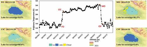
In several earlier studies (Kang et al., 2011, 2014; Wang et al., 2019), the dates of the first freezing and thawing of a lake were denoted as the FO and MO dates, respectively; the dates of the first complete freezing of a lake and the surface being completely ice-free were denoted as the CIC and CIF dates. In this study, we used an empirical change-detection method to track the lake ice phenology. We defined the FO date as the last date before the sudden increase of brightness temperature from the open-water value. The CIC date was determined in the following way. Following the FO date, there is a steady and continuous increase in the brightness temperature. This process generally lasts for several weeks or months depending on the climate zone in which the lake is located. We defined the CIC date as being the first date belonging to this period. The MO date was considered to coincide with the drop in brightness temperature that occurs at the end of the freezing period. The first date of the continuous and monotonous decrease in brightness temperature was taken as the MO date and the last date of this fall as the CIF date. After the CIF date, there is usually an ice-free period that lasts until the next freezing season. Figure 3 illustrates the determination of the FO, CIC, MO and CIF dates using the example of Hala Lake, which is located on the Tibetan Plateau at 97.59 °E, 38.29 °N. MODIS images corresponding to these dates are also shown.

Figure 3. Time-series of brightness temperatures extracted from the PMW data for the period August 2013 to July 2014 at Hala lake. The four MODIS images illustrate the surface ice coverage corresponding to the FO, CIC, MO and CIF dates.

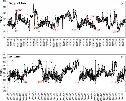
Using the method that has been described, ice phenology parameters for 753 lakes were extracted from PMW data. However, for some lakes, some of the parameters were difficult to extract because of fluctuations in the brightness temperature signals (Figure 4). In such cases, we left the parameters undetermined and denoted them as NaN.

Figure 4. Multi-seasonal brightness temperature time-series for (a) Kayigyalik lake and (b) the lake Hy_ID555, where it proved difficult to identify some of the ice phenology parameters. The surface areas of these lakes are 139.5 km² and 138.5 km², respectively, and the lakes are located at (162.5 °W, 61.1 °N) and (92.6 °W, 54.5 °N).

2.3. Technical validation

The Global Lake and River Ice Phenology Database provided by the NSIDC only records ice-on and ice-off dates (Benson et al., 2000). Ground observation records from 20 lakes were selected (Table S1) and comparisons were made between the ice-on dates and the CIC dates that had been determined and between the ice-off dates and the extracted CIF dates (Figure 5). For the relationship between the CIC and ice-on dates, the correlation coefficient is 0.93 (P < 0.001) with an RMSE of 11.84 days and a bias of 9.34 days; between the CIC and ice-off dates, the correlation coefficient is 0.84 (P < 0.001) with an RMSE of 10.07 days and a bias of 8.03 days.

Figure 5. Comparison between (a) the CIC and (b) CIF dates identified from the PMW data and the corresponding values from the NSIDC’s GLRIPD.

The ice phenology data for fifteen lakes (Table S2) were randomly selected from the 308 sets of lake ice phenology results obtained from the MODIS data (Qiu et al., 2019). The dates when the lake ice area accounted for 10% and 90% of the entire lake were considered as the FO/CIF and CIC/MO dates, respectively (Reed, Budde, Spencer, & Miller, 2009). The verification results show (Figure 6) that the lake ice phenology results obtained from the MODIS and PMW data are highly correlated (P < 0.001). The average RMSE is 7.865 days; the CIF has the smallest RMSE and bias at 4.39 days and 3.86 days, respectively. Although there is significant correlation between the two sets of results, MODIS observations are not perfect. Therefore, third-party databases should be used as much as possible for verification.

Figure 6. Verification of the lake ice phenology results: results extracted from MODIS data plotted (y-axis) against results extracted from PMW (x-axis) data for (a) the FO, (b) the CIC, (c) the MO and (d) the CIF dates, respectively.

3. Data records

The lake ice phenology results derived from the PMW data were stored in Excel format under the name Lake ice phenology dataset for Northern Hemisphere.xls. For this excel file, the Physical character records lake attributes and each numbered table represents a different lake. The format used is showed in Table 2.

Table 2. Dataset attribute descriptions.

Table	Parameter	Description
Physical character	This table details the attributes of lakes with monitoring records.
	ID	Unique dataset identifier
	hy_id	The number of the lake in the HydroLAKES database
	Name*	The name of the lake
	Sample center_lat	Sampling point latitude
	Sample center_long	Sampling point longitude
	Area*	Lake surface area in square kilometers
	Altitude*	The elevation of the lake surface in meters
	Vol_total*	The total volume of the lake in millions of cubic meters
	Depth_avg*	The average depth of the lake in meters
	Country*	The country where the lake is located
	Continent*	The continent where the lake is located
	PMW_year	The start and end years for the PMW monitoring
	Ob_year	The start and end years of the ground observation records
	NSIDC_lake code	Lake observation station (from the NSIDC)
	MODIS_Ob	Whether the lake ice extent was obtained from MODIS data: Y = yes, N = no
xxx Lake	lake ice phenology records can be found for the lake with ID xxx
	Season	The ice season given in the form YYYY, where YYYY is the year
	Freeze Onset	Freeze Onset: the date on which the sampling point first freezes – given in YYYY, M, D format, where YYYY is the year, M (1 or 2 digits) is the month and D is the day (1 or 2 digits)
	Complete Ice Cover	Complete Ice Cover: the date on which the sampling point first appears to be completely frozen – given in YYYY, M, D format
	Melt Onset	Melt Onset: the date on which the snow on the surface of the ice begins to melt – given in YYYY, M, D format
	Complete Ice Free	Complete Ice Free: the date on which the sampling point first appears to be completely free of ice – given in YYYY, M, D format

*Records from the HydroLAKES database.

In the dataset that was produced (Table 3), the lake ice phenology was obtained for 753 Northern Hemisphere lakes distributed across 15 countries on three continents (Asia, Europe, and North America). 485 of the lakes are located in North America, mainly between 50 °N and 65 °N (413 of 485 records). The numbers of lakes located in Europe and Asia are 116 and 152, respectively; the Eurasian lakes are concentrated on the Tibetan Plateau and in the zone 45 °N–65 °N (242 of 268 records). There are 88, 78, 383, 129 and 75 lakes with areas of more than 1000 km², 500–1000 km², 100–500 km², 50–100 km², and less than 50 km², respectively. For the period 2002 to 2020, lakes with an area of 50 between 500 km² were the most numerous, totaling 276 lakes. This is mainly affected by the number of lakes and the resolution of the remote sensing data.

Table 3. Statistics of the lakes in the dataset.

Spatial unit	Number of lakes		Average Area (km^2)	Average depth (m)	Average volume (km^3)	Average elevation (m)	Number of ground stations
	(1978–2020)	(2002–2020)
Size class (km^2)
< 50	38	37	43.93	8.02	0.35	786.68	0
50–100	42	87	68.49	9.57	0.67	1685.55	0
100–500	194	189	250.84	16.36	4.38	870.17	22
500–1000	61	17	715.87	15.97	11.58	547.35	10
> 1000	74	14	4,253.97	31.30	381.70	394.44	22
Continent
Asia	46	106	502.52	14.88	9.91	3,481.35	1
Europe	47	69	1,244.52	20.58	223.45	135.34	21
North America	316	169	654.93	15.37	18.26	293.31	32
Lake data by country
Canada	298	154	619.19	15.72	17.99	296.94	30
China	28	89	272.51	13.49	5.05	4,134.06	1
Russia	34	55	1,420.86	22.14	288.84	143.42	13
United States of America	17	14	1,211.64	8.58	23.04	228.42	2
Finland	10	6	741.16	16.41	8.58	84.38	8
Lake data by latitude range
28.57 °N–35 °N	12	61	223.99	17.07	5.75	4,693.92	0
35 °N–40 °N	10	23	301.08	12.48	5.18	4,421.94	1
40 °N–45 °N	5	9	2,463.17	13.72	41.16	1,262.43	2
45 °N–50 °N	32	34	980.00	12.88	14.55	503.55	2
50 °N–55 °N	74	86	917.41	18.41	161.23	350.74	17
55 °N–60 °N	88	59	558.16	13.87	10.39	261.87	12
60 °N–65 °N	156	52	602.95	16.52	19.84	209.93	14
65 °N–74.5 °N	32	20	1,128.65	18.94	52.01	179.83	6

4. Discussion

4.1. Analysis of changes in lake ice phenology

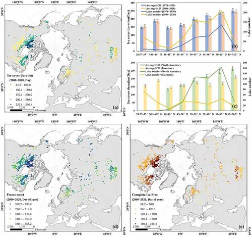
Using the FO and CIF dates, the duration of ice cover for each lake was calculated and the results for two different periods – 1978 to 1999 and 2000 to 2020 – were analyzed. In terms of the spatial variation in the results (Figure 7(a,d,e)), it can be seen that, as the latitude increases, the freezing events occur earlier and the melting events occur later, meaning that the ice-cover duration becomes longer. The most southerly of the lakes in the dataset that was found to freeze was Lake Puma Yumco (90.40 °E, 28.57 °N), which is located on the Tibetan Plateau. Analysis of the average FO and CIF dates for the period after 2000 (parts (d) and (e)), showed that the freezing and thawing dates were consistent with each other – that is, the lakes that freeze early will melt later. The bar graph (Figure 7(b)) shows that the ice-cover duration for lakes with latitudes in the range 28 °N–40 °N is longer than for those in the range 40 °N–45 °N and even longer than for those in the range 45 °N–50 °N. This is because the low-latitude lakes are mostly located on the Tibetan plateau. The ice-cover duration is longer around Hudson Bay and on the northern Tibetan Plateau (about 35 °N–40 °N) than in other regions at the same latitudes. North of 45 °N, the average ice-cover duration is longer for North American lakes than for Eurasian lakes (Figure 7(c)) at the same latitude.

Figure 7. Spatial patterns in the lake ice phenology results: (a), (d), and (e) show the average ice cover duration, the average FO date, and the average CIF date, respectively, during the period 2000 to 2020. (b) and (c) show statistics for the ice-cover duration by region.

4.2. Challenges in monitoring lake ice phenology based on PMW

The use of the nearest neighbor algorithm to obtain lake ice phenology has some limitations. The algorithm considers that the freezing and melting dates of the lake center apply to the whole lake. In general, the freezing and melting of a lake start from the lakeshore, where the water is shallow and cooling is rapid (Leppäranta, 2015). The freezing and thawing are affected not only by the air temperature but also by the amount of solar radiation, the shape of the lake, the basin topography, precipitation, wind, and other factors. Therefore, there can be spatial variations in freeze–thaw processes that will not detected by the proposed method. For example, Nam Co (area 1,982 km²) is the second largest lake on the Tibetan Plateau, and it freezes from east to west in winter (Gou et al., 2017). Ice formation in the Great Slave Lake (area 27,200 km²) is affected by the flow of the Slave River into the southeastern part of the lake, which causes late freezing and early melting in that part (Howell, Brown, Kang, & Duguay, 2009). Therefore, to improve the proposed method, it would be necessary to make observations of the entire lake instead of just the center.

Moreover, the inherent coarse spatial resolution of PMW sensors means that observations of lakes are contaminated by land in many cases. However, we determined that the lake freezing signals were sufficiently strong to overcome the influence of mixed pixels. Scenes that were possibly problematic were identified during the determination of the lake ice phenology (section 2.2.3). The use of different data sources may lead to differences in the interpretation of lake ice phenology. Although the same algorithm for extracting the lake ice phenology can be used with these different sources, it will be necessary to calibrate the brightness temperature data if the extraction algorithm is automated in future.

According to the HydroLAKES database and the location of the 0°C isotherm in January (Brooks, Prowse, & O’Connell, 2013), there are 1,263.4 × 10³ frozen lakes (including Greenland) with areas of less than 50 km² in northern hemisphere (Table 4), these lakes cover a total area of about 876.8 × 10³ km² and account for 32.84% of the total area covered by lakes globally. In future work, we plan to include an analysis of these smaller lakes.

Table 4. Statistics on the number of frozen lakes with areas less than 50 km^2.

Area (km^2)	Asia	Europe	North America	Total number	Total area (km^2)
0.1–1	22.3 × 10^3	225.0 × 10^3	860.9 × 10^3	1,108.2 × 10^3	307.3 × 10^3
1–10	6.7 × 10^3	42.9 × 10^3	95.1 × 10^3	144.7 × 10^3	359.4 × 10^3
10–20	548	1,863	4,433	6,844	94.2 × 10^3
20–30	293	506	1,215	2,014	55.2 × 10^3
30–40	116	250	631	997	34.4 × 10^3
40–50	85	152	357	594	26.5 × 10^3
Total number	30.1 × 10^3	270.7 × 10^3	962.7 × 10^3	1,263.4 × 10^3	NA
Total area (km^2)	50.5 × 10^3	231.4 × 10^3	594.9 × 10^3	NA	876.8 × 10^3

5. Conclusions

The ice phenology of 753 lakes in the Northern Hemisphere was retrieved from the passive microwave remote sensing data. This dataset is composed of two parts: observations of 409 lakes for 1978–2020 and observation of 344 lakes for 2002–2020. Verification of the data against ground observations and optical remote sensing data showed that the PMW LIP dataset has an acceptable accuracy. The PMW LIP data complement the ground observations and lake ice phenology records made in the Northern Hemisphere over the past 40 years. However, lakes with an area of less than 40 km² are not included in the current dataset. These smaller lakes will be the subject of future work, where a model-based approach will be used to reduce the influence of lakeshore pixels.

Our analysis of lake ice phenology showed that the ice cover duration has a latitudinal distribution, that is, the duration becomes longer as the latitude increases. Lakes in the Hudson Bay region and on the northern Tibetan Plateau have longer ice cover than lakes at the same latitude elsewhere. North of 45 °N, North American lakes have longer ice-cover periods than Eurasian lakes at similar latitudes. These phenomena are due to the effects of the regional climate. Analysis of this long time-series of lake ice phenology revealed that, across the Northern Hemisphere, lakes are tending to freeze later and melt earlier, which corroborates the results of earlier studies.

This dataset is publicly available. Users can obtain the ice cover duration for lakes based on the FO and CIF dates, and the complete ice cover duration based on the CIC and MO dates. The dataset will be updated every 1–2 years.

Disclosure statement

No potential conflict of interest was reported by the author(s).

Data availability statement

The dataset is openly available from the repository located at http://www.doi.org/10.11922/sciencedb.j00076.00081.

Supplementary material

Supplemental data for this article can be accessed here.

Additional information

Funding

This study was supported by the the Multi-Parameters Arctic Environmental Observations and Information Services Project (MARIS) funded by Ministry of Science and Technology (MOST) [grant number 2017YFE0111700] and Strategic Priority Research Program of the Chinese Academy of Sciences [grant numbers XDA19070201 and XDA19070102].

Notes on contributors

Xingxing Wang

Xingxing Wang is a Ph.D. candidate in geography at Northwestern University, China. She has focused on the application of remote sensing to the monitoring of lake ice since 2016. She was a visiting young scientist with Aerospace Information Research Institute, Chinese Academy of Science (AIR, CAS) , Beijing, China. Her research topic is in the field of disaster science.

Yubao Qiu

Dr. Yubao Qiu is a full professor at the Aerospace Information Research Institute, Chinese Academy of Sciences (AIR, CAS) and International Research Center of Big Data for Sustainable Development Goals, Beijing, China. His main research interests include microwave remote sensing, remote sensing of snow and ice, and its applications in Arctic and High Mountain Asia (HMA). Dr. Qiu was an expert on the Secretariat to the Group on Earth Observations (GEO), Geneva, Switzerland, from 2012 to 2015. Over the past five years, he has published more than 70 papers.

Yixiao Zhang

Yixiao Zhang is a master’s degree candidate in resources and environment at the Aerospace Information Research Institute, Chinese Academy of Sciences. Her research interests focus on geoscience using remote sensing.

Juha Lemmetyinen

Juha Lemmetyinen has over ten years of experience in the field of Earth observations. His background includes microwave radiometer engineering, radiometer calibration techniques as well as active and passive remote sensing applications. He has been with the Finnish Meteorological Institute (FMI) since 2008, specializing in the modeling of microwave signatures and the development of retrieval algorithms for active and passive microwave remote sensing with a focus on cryosphere applications.

Bin Cheng

Bin Cheng is a Senior scientist at the Finnish Meteorological Institute (FMI). His research interests focus on the thermodynamic modeling of snow and ice, air–ice–sea interactions, operational snow and ice analysis and forecasting, sea-ice dynamics and thermodynamic coupling, and snow and ice modeling in remote sensing applications.

Wenshan Liang

Wenshan Liang is an engineer on GIS and remote sensing, and was with in the Aerospace Information Research Institute, Chinese Academy of Sciences. Her research interests mainly focus on the monitoring of river ice using remote sensing.

Matti Leppäranta

Matti Leppäranta is a full professor at Helsinki University, Finland. His research interests cover the geophysics of sea ice and lake ice – including ice structure and morphology – remote sensing, thermodynamics, dynamics and environmental and climate questions. He retired in 2018 but has continued his research as an emeritus professor at the university.

References

- Beck, H., Zimmermann, N., McVicar, T., Vergopolan, N., Berg, A., & Wood, E. (2018). Present and future Köppen-Geiger climate classification maps at 1-km resolution. Scientific Data, 214(5), 180214.111.
- Benson, B., Magnuson, J., & Sharma, S. (2000). updated 2020. Global lake and river ice phenology database, version 1. [Indicate subset used]. Boulder, Colorado USA. NSIDC: National Snow and Ice Data Center. doi: 10.7265/N5W66HP8.
- Brodzik, M. J., Long, D. G., Hardman, M. A., Paget, A., & Armstrong, R. (2016), Updated 2020. MEaSUREs calibrated enhanced-resolution passive microwave daily EASE-grid 2.0 brightness temperature ESDR, version 1. [Indicate subset used]. boulder, Colorado USA. NASA National Snow and Ice Data Center Distributed Active Archive Center. doi: 10.5067/MEASURES/CRYOSPHERE/NSIDC-0630.001.
- Brooks, R. N., Prowse, T., & O’Connell, I. J. (2013). Quantifying Northern Hemisphere freshwater ice. Geophysical Research Letters, 40(6), 1128–1131.
- Cai, Y., Ke, C., Li, X., Zhang, G., Duan, Z., & Lee, H. (2019). Variations of lake ice phenology on the Tibetan Plateau from 2001 to 2017 based on MODIS data. Journal of Geophysical Research, 124, 825–843.
- Canadian Cryospheric Information Network. Canadian lake ice database [EB/OL]. (November 13, 2017). Accessed 2021 February 26. Retrieved from https://www.polardata.ca/pdcsearch/PDCSearch.jsp?doi_id=1821
- Denfeld, B., Baulch, H., Giorgio, P., Hampton, S., & Karlsson, J. (2018). A synthesis of carbon dioxide and methane dynamics during the ice-covered period of northern lakes. Limnology and Oceanography, 3(3), 117–131.
- Du, J., Kimball, J. S., Duguay, C., Kim, Y., & Watts, J. D. (2017). Satellite microwave assessment of Northern Hemisphere lake ice phenology from 2002 to 2015. The Cryosphere, 11(1), 47–63.
- Duguay, C. R., Prowse, T. D., Bonsal, B., Brown, R., Lacroix, M. P., & Menard, P. (2006). Recent trends in Canadian lake ice cover. Hydrological Processes, 20(4), 781–801.
- Filazzola, A., Blagrave, K., Imrit, M., & Sharma, S. (2020). Climate change drives increases in extreme events for lake ice in the Northern Hemisphere. Geophysical Research Letters, 47(18), e2020GL089608.
- Gloersen, P., & Barath, F. (1977). A scanning multichannel microwave radiometer for Nimbus-G and SeaSat-A. IEEE Journal of Oceanic Engineering, 2(2), 172–178.
- Gou, P., Ye, Q., Che, T., Feng, Q., Ding, B., Lin, C., & Zong, J. (2017). Lake ice phenology of Nam Co, Central Tibetan Plateau, China, derived from multiple MODIS data products. Journal of Great Lakes Research, 43(6), 989–998.
- Guo, H., Li, X., & Qiu, Y. (2020). Comparison of global change at the Earth’s three poles using spaceborne earth observation. Chinese Science Bulletin, 65, 1320–1323.
- Hollinger, J. P., Peirce, J. L., & Poe, G. A. (1990). SSM/I instrument evaluation. IEEE Transactions on Geoscience and Remote Sensing, 28(5), 781–790.
- Howell, S., Brown, L. C., Kang, K., & Duguay, C. (2009). Variability in ice phenology on great bear lake and great slave lake, Northwest Territories, Canada, from SeaWinds/QuikSCAT: 2000-2006. Remote Sensing of Environment, 113(4), 816–834.
- Kang, K., Duguay, C., & Howell, S. (2011). Estimating ice phenology on large northern lakes from AMSR-E: Algorithm development and application to great bear lake and great slave lake, Canada. The Cryosphere, 6(2), 235–254.
- Kang, K., Duguay, C., Lemmetyinen, J., & Gel, Y. (2014). Estimation of ice thickness on large northern lakes from AMSR-E brightness temperature measurements. Remote Sensing of Environment, 150, 1–19.
- Karetnikov, S., Leppäranta, M., & Montonen, A. (2017). A time series of over 100 years of ice seasons on lake Ladoga. Journal of Great Lakes Research, 43(6), 979–988.
- Kawanishi, T., Sezai, T., Ito, Y., Imaoka, K., Takeshima, T., Ishido, Y., … Spencer, R. (2003). The Advanced Microwave Scanning Radiometer for the Earth Observing System (AMSR-E), NASDA’s contribution to the EOS for global energy and water cycle studies. IEEE Trans. Geosci. Remote. Sensing, 41(2), 184–194.
- Kropácek, J., Maussion, F., Chen, F., Hoerz, S., & Hochschild, V. (2013). Analysis of ice phenology of lakes on the Tibetan Plateau from MODIS data. The Cryosphere, 7(1), 287–301.
- Latifovic, R., & Pouliot, D. (2007). Analysis of climate change impacts on lake ice phenology in Canada using the historical satellite data record. Remote Sensing of Environment, 106(4), 492–507.
- Leppäranta, M. (2015). Freezing of lakes and the evolution of their ice cover, (chapter 1, pp.1-10; chapter 2, pp.11-50; chapter 3, 51-90). In Leppäranta M. (Ed.). Springer-Praxis. Germany: Heidelberg.
- Li, X., Che, T., Wang, L., Duan, A., Shangguan, D., Pan, X., Fang, M., & Bao, Q. (2020). CASEarth Poles: Big Data for the Three Poles. Bulletin of the American Meteorological Society, 101, E1475–E1491.
- Long, D., Brodzik, M., & Hardman, M. (2019). Enhanced-resolution SMAP brightness temperature image products. IEEE Transactions on Geoscience and Remote Sensing, 57(7), 4151–4163.
- Lu, J., Qiu, Y., Wang, X., Liang, W., Xie, P., Shi, L., … Zhang, D. (2020). Constructing dataset of classified drainage areas based on surface water-supply patterns in High Mountain Asia. Big Earth Data, 4(3), 225–241.
- Maeda, T., Imaoka, K., Kachi, M., Fujii, H., Shibata, A., Naoki, K., … Oki, T. (2011). Status of GCOM-W1/AMSR2 development, algorithms, and products. SPIE Remote Sensing, 8176, 6012–6015.
- Magnuson, J. J., Robertson, D. M., Benson, B. J., Wynne, R. H., Livingstone, D. M., Arai, T., … Vuglinski, V. S. (2000). Historical trends in lake and river ice cover in the Northern Hemisphere. Science, 289(5485), 1743–1746.
- Messager, M. L., Lehner, B., Grill, G., Nedeva, I., & Schmitt, O. (2016). Estimating the volume and age of water stored in global lakes using a geo-statistical approach. Nature Communications, 7(1), 13603.
- National centers for environmental information [EB/OL]. (2017). Accessed 2021 April 30. https://www.ncdc.noaa.gov/gosic/gcos-essential-climate-variable-ecv-data-access-matrix/gcos-land-ecv-lakes
- Qiu, Y., Guo, H., Ruan, Y., Fu, X., Shi, L., & Tian, B. (2017). A dataset of microwave brightness temperature and freeze-thaw for medium-to-large lakes over the High Asia region 2002–2016. Science Data Bank. doi:10.11922/csdata.170.2017.0117
- Qiu, Y., Massimo, M., Li, X., Birendra, B., Joni, K., Narantuya, D., … Zhao, T. (2017). Observing and understanding High Mountain and cold regions using Big Earth Data. Bulletin of Chinese Academy of Sciences, 32(Z1), 82–94.
- Qiu, Y., Xie, P., Leppäranta, M., Wang, X., Lemmetyinen, J., Lin, H., & Shi, L. (2019). MODIS-based daily lake ice extent and coverage dataset for Tibetan Plateau. Big Earth Data, 3(2), 170–185.
- Reed, B., Budde, M., Spencer, P., & Miller, A. E. (2009). Integration of MODIS-derived metrics to assess interannual variability in snowpack, lake ice, and NDVI in southwest Alaska. Remote Sensing of Environment, 113(7), 1443–1452.
- Ruan, Y., Zhang, X., Xin, Q., Qiu, Y., & Sun, Y. (2020). Prediction and analysis of lake ice phenology dynamics under future climate scenarios across the Inner Tibetan Plateau. Journal of Geophysical Research, 125, e2020JD033082.
- Sharma, S., Blagrave, K., Magnuson, J., O’Reilly, C., Oliver, S., Batt, R., … Woolway, R. (2019). Widespread loss of lake ice around the Northern Hemisphere in a warming world. Nature Climate Change, 9(3), 227–231.
- Sharma, S., Meyer, M., Culpepper, J., Yang, X., Hampton, S., Berger, S. A., … Zhang, S. (2020). Integrating perspectives to understand lake ice dynamics in a changing world. Journal of Geophysical Research, 125, e2020JG005799.
- Šmejkalová, T., Edwards, M. E., & Dash, J. (2016). Arctic lakes show strong decadal trend in earlier spring ice-out. Scientific Reports, 6(1), 38449.
- Su, L., Che, T., & Dai, L. (2021). Variation in ice phenology of large lakes over the Northern Hemisphere based on passive microwave remote sensing data. Remote Sensing, 13(7), 1389.
- Ulaby, F., Moore, R., & Fung, A. (1981). Microwave remote sensing fundamentals and radiometry.
- Wang, X., Qiu, Y., Xie, P., Lemmetyinen, J., Liang, W., & Cheng, B. (2019). Comparative analysis to the lake ice phenology changes of Mongolian Plateau, Tibetan Plateau and Northern Europe through passive microwave. 2019 Photonics & Electromagnetics Research Symposium - Fall (PIERS - Fall, Xia'men, China), 3222–3228.
- Woolway, R., Kraemer, B., Lenters, J., Merchant, C., O’Reilly, C., & Sharma, S. (2020). Global lake responses to climate change. Nature Reviews Earth & Environment, 1(8), 388–403.
- Wu, Y., Duguay, C., & Xu, L. (2020). Assessment of machine learning classifiers for global lake ice cover mapping from MODIS TOA reflectance data. Remote Sensing of Environment, 253(5), 112206.
- Yang, H., Weng, F., Lv, L., Lu, N., Liu, G., Bai, M., … Xu, H. (2011). The FengYun-3 microwave radiation imager on-orbit verification. IEEE Transactions on Geoscience and Remote Sensing, 49(11), 4552–4560.
- Yang, J., Dong, C., Lu, N., Yang, Z., Shi, J., Zhang, P., … Cai, B. (2009). FY-3A: The new generation Polar-Orbiting meteorological satellite of China. Acta Meteorologica Sinica, 67(4), in Chinese, 501–509.
- Zhang, G., Yao, T., Xie, H., Yang, K., Zhu, L., Shum, C., … Ke, C. (2020). Response of Tibetan Plateau lakes to climate change: Trends, patterns, and mechanisms. Earth-Science Reviews, 208, 103269.
- Zhang, S., & Pavelsky, T. (2019). Remote sensing of lake ice phenology across a range of lakes sizes, ME, USA. Remote Sensing, 11(14), 1718.