Generating high-resolution climatological precipitation data using SinGAN

ABSTRACT

High-resolution (HR) climate data are indispensable for studying regional climate trends, disaster prediction, and urban development planning in the face of climate change. However, state-of-the-art long-term global climate simulations do not provide appropriate HR climate data. Deep learning models are often used to obtain high-resolution climate data. However, due to the fact that these models require sufficient low-resolution (LR) and HR data pairs for the training process, they cannot be applied to scenario with inadequate training data. In this paper, we explore the applicability of a single image generative adversarial network (SinGAN) in generating HR climate data. SinGAN relies on single LR input data to obtain the corresponding HR data. To improve the performance for extreme-value regions, we propose a SinGAN combined with the weighted patchGAN discriminator (WSinGAN). The proposed WSinGAN outperforms comparable models in generating HR precipitation data, and its results are close to real HR data with sharp gradients and more refined small-scale features. We also test the scalability of the pre-trained WSinGAN for unseen samples and show that although only a single LR sample is used to train WSinGAN, it can still produce reliable HR data for unseen data.

KEYWORDS:

• Climate downscaling
• SinGAN
• deep learning
• adversarial training

1. Introduction

High-resolution (HR) climate data are of great importance to climate-related research. More specifically, HR climate data help to improve our understanding of the impacts of climate change on a regional scale, as well as provide accurate natural disaster prediction and disaster mitigation planning. One of the most commonly used sources of climate data in current studies is the global climate model (GCM), a physics-based numerical model that simulates dynamic systems that couple atmospheric, terrestrial, and oceanic processes (Bonan & Doney, 2018; Schiermeier, 2010). These models provide climate data on a coarse spatial scale, typically between 1 and 3 degrees, a resolution so coarse that we are unable to investigate related climate change patterns on a small scale for both historical and future climate scenarios. In addition, because the relevant scale-specific physics, computational resources, and time frames associated with each application are customized into numerical models, simulating all relevant scales is generally problematic. Consequently, flexible access to HR climate data on different scales is needed for different scenarios.

Downscaling techniques are used to improve low-spatial resolution through modeling. Dynamical downscaling is a physics-based downscaling method, which drives regional climate models with low-resolution (LR), large-scale climate data to obtain HR, small-scale climate data (Frey-Buness et al., 1995; Rockel et al., 2008). Similar to GCM, dynamic downscaling is computationally demanding and untransferable across regions. Another method is statistical downscaling, a data-driven approach (Wilby et al., 1998) to obtain HR climate data by establishing a statistical relationship between HR and LR pairs, which is not restricted to the human understanding of the problem and does not involve solving complicated systems of equations. In past studies, linear regression models (Huth, 2002), support vector machines (Chen et al., 2010), and random forests (Yang et al., 2017, Hutengs et al., 2016) have been applied to establish statistical relationships between HR and LR data. Generating HR climate data is similar to what is known as single image super-resolution (SISR) in computer vision (Yang et al., 2019). The goal of SISR is to address the problem of resolving an HR image from its LR counterpart, but it remains a classic ill-posed problem and one of the most active research areas since Tsai and Huang’s work in 1984. With the extensive development of deep learning, a growing number of related models have been used to solve the SISR problem. For example, the super-resolution convolutional neural network (SRCNN) was the first super-resolution CNN (Dong et al., 2015), and very deep super-resolution (VDSR) increases the depth of the SRCNN from three to 20 layers (Kim et al., 2016). Further, generative adversarial networks (GANs) are used to solve the SISR problem (Ledig et al., 2017; Wang et al., 2018), and deep learning models have been developed as a promising technique for overcoming SISR. Naturally, this has raised interest in exploring how these approaches may be applied to climate data. Rocha Rodrigues et al. (2018) proposed a deep neural network-based strategy to learn HR representations from LR predictions. Their results show that this strategy can obtain better HR data with a lesser computational cost. Further, Vandal et al. (2017) constructed deep statistical downscaling (DeepSD) based on a stack of two SRCNNs. They used DeepSD to downscale the precipitation data from 1 degree (100 km) to 1/8 degree (12.5 km), and the results show that DeepSD can provide ideal HR precipitation data. Cheng et al., 2020 generated HR climate data using a GAN, which performed better than most super-resolution approaches in climate prediction. Stengel et al. (2020) also used a GAN to obtain HR climatological wind and solar data, where, through experiments, they increased the resolution of the raw data by a factor of 50.

However, we found that all the deep learning models used so far are mainly supervised learning models, which means that sufficient training data, i.e. LR and HR data pairs, are necessary to achieve high-quality results (Chen & Lin, 2014). HR climate data cannot be generated by existing models when training data are insufficient. To overcome this problem, a new single-image GAN (SinGAN) model in computer vision has been proposed. SinGAN can effectively capture and access the internal relationship of an input training image in the absence of a significant number of training samples. First proposed by Shaham et al. (2019) as an unconditional generative model, SinGAN relies only on a single natural image. SinGAN employs a series of GANs to generate real images that progress from coarse to detailed and from LR to HR. Through a pyramidal structure, SinGAN learns the internal distribution within a single natural image; thus, the model can capture the global structure, as well as detailed information of the image, including its texture. SinGAN can be used for different image manipulation tasks, such as super-resolution, paint-to-image, editing, and single image animation, a number of studies on SinGAN have been conducted in the field of computer vision. Sun and Liu (2020) proposed the enhanced single-image GAN (ESinGAN) by combining SinGAN and a pixel attention mechanism. Their results show that ESinGAN can improve the performance of SinGAN on super-resolution images. To solve the problem of insufficient training data for remote sensing images, Gu et al. (2021) combined SinGAN and an attentional mechanism to generate pseudo samples with stronger realism while requiring only minimal training data. Further, Cheng et al. (2020) applied SinGAN to generate HR rock-thin section images, and Xinwei et al. (2021) transformed SinGAN into a conditional GAN to make images more clearer in terms of spatial layout and semantic information.

As SinGAN is increasingly being used to solve the SISR problem, in this paper, we investigate the applicability of SinGAN for generating HR climate data. SinGAN obtains enough information to build a robust model through adversarial learning of the internal statistics of patches within a single sample, meaning that it can obtain corresponding HR data using a single LR input. This feature can help us solve the problem of obtaining HR climate data from insufficient training data. Besides, for climate data, extreme-value regions are of great research importance, as they often face extreme climate events and natural disasters (Tank et al., 2009). Traditional statistical scaling methods tend to smooth the values in these regions. To improve the simulation results of the model for extreme-value regions, we modified the discriminator in the original SinGAN to a weighted patchGAN discriminator. For convenience, we refer to our proposed SinGAN with the weighted patchGAN discriminator simply as WSinGAN in the remainder of this manuscript. We experimentally verify the applicability of WSinGAN to the generation of HR climatological precipitation data, and we verify the temporal and spatial scalability of the pre-trained WSinGAN for unseen samples.

The structure of the paper is as follows: Section 2 introduces the model structure of SinGAN. On this basis, the loss function of the model is discussed, and the proposed weighted patchGAN discriminator is discussed. Section 3 presents the data used in the paper and the evaluation metrics, and Section 4 describes the results. The paper concludes with a discussion in Section 5 and concluding remarks in Section 6.

2. Methodology

2.1. Structure of SinGAN

SinGAN takes advantage of commonly used GAN models, which mainly utilize the adversarial learning approach. Figure 1 shows that GAN models are composed of two parts: a generator $G$ and a discriminator $D$. The role of the generator $G$ is to generate fake samples from random noise, while the discriminator $D$ tries to distinguish between the input coming from real and fake samples. Through this adversarial learning, the distribution of fake samples generated by the generation model $G$ approaches the distribution of real samples more closely.

Figure 1. The framework structure of generative adversarial networks (GANs).

Unlike traditional GANs, which are composed of only one generator and one discriminator, SinGAN is composed of a series of generators and discriminators (Figure 2), where each generator $\left\{G_n,G_{n-1},...,G_1,G_0\right\}$ is trained against its corresponding discriminator $\left\{D_n,D_{n-1},...,D_1,D_0\right\}$. SinGAN has a pyramidal structure with $G_n$ and $D_n\mathrm{a}\mathrm{s}$ the lowest-level generator and discriminator, and $G_0$ and $D_0$ as the highest-level generator and discriminator $G_0$ and $D_0$, respectively. As previously mentioned, SinGAN does not require a training dataset; it is trained based on only a single training sample. For example, if the model needs to increase the resolution of the input by a factor of $r>1$ through $n$ generator and discriminator pairs, during the training process, the single input sample is first downsampled to different scales $\left\{rea{l}_n,rea{l}_{n-1},...,rea{l}_1,rea{l}_0\right\}$ by a factor of $r^n$. In each layer of SinGAN, the discriminator learns to distinguish between $fak{e}_n$ and $rea{l}_n$, while the generator learns how to obtain $fak{e}_n$ from the input, which can confuse the discriminator’s judgment. The lowest-level generator’s input is simply spatial white Gaussian noise, $nois{e}_n$. Except for the lowest-level generator, the generators of the other layers contain two parts: the spatial white Gaussian noise, $nois{e}_n,$ and the upsampled version of $fak{e}_{n+1}$:

Figure 2. The structure of SinGAN. SinGAN model consists of a pyramid of GANs, where $G_n$ and $D_n$ are the lowest-level generator and discriminator $G_n$ and $D_n$, $G_0$ and $D_0$ are the highest-level generator and discriminator $G_0$ and $D_0$, respectively.

$fak{e}_n=\left\{\begin{array}{c}{G}_n\left(nois{e}_n\right),n=N\\ G_n\left(nois{e}_n,upsample{d}_n\right),n<N\end{array}\right..$

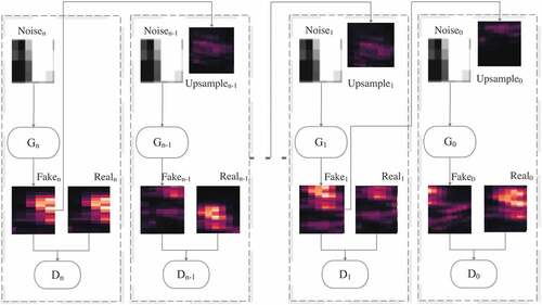
The process of training SinGAN can be viewed as learning the transformation from 1/$r$ of the original resolution to the original resolution. When the training process is completed, the result of increasing the original resolution by a factor of $r$ can be obtained if we input the original resolution data into the model. In the step from a low-level to a high-level GAN, the results gradually move from coarse to fine scales. In coarse scales, SinGAN focuses on the global information of the input, such as shape, while in fine scales, SinGAN pays greater attention to detailed information, such as texture and edge.

All generators have the same structure: a fully convolutional layer with five blocks of Conv(3 × 3)-BatchNorm-leakyReLU (Ioffe & Szegedy, 2015). Because the data we use have only one channel corresponding to precipitation, it is different from the three RGB channels of an image. We adjust the input channel to be one channel, and we use the same kernel size as the original SinGAN. Starting at a coarse scale with a kernel size of 32, the kernel size increases by a factor of two every four scales. The patchGAN discriminator is used in the model, and we discuss its details in the following section. We also use the same patch size as the original SinGAN (11 × 11) in different layers of the GAN, which means on the coarse scale, the patch size covers a large area of the input, while on a finer scale, the patch size covers a smaller area of the input. The former helps the model capture global properties, while the latter aids in the model’s awareness of more detailed information.

2.2. Loss function and the weighted patchGAN discriminator

SinGAN is trained from the lowest $\left(G_n,D_n\right)$ to the highest levels $\left(G_0,D_0\right)$ sequentially. Each level remains fixed upon completion of the training, and each GAN layer has the same loss function, which includes adversarial loss $L_{adv}$ and reconstruction loss $L_{rec}$:

$\underset{G_n}{min}\underset{D_n}{max}{L}_{adv}\left(G_n,D_n\right)+\alpha L_{rec}\left(G_n\right).$

Reconstruction loss, $L_{rec}$, compares the difference between the generated HR $fak{e}_n$ data and the corresponding $rea{l}_n$ data and adjusts the parameters of the generator for the input data at each scale. Its coefficient $\alpha$ is set to 30 in this work, and the reconstruction loss is calculated as follows:

$L_{rec}=\left\{\begin{array}{c}\parallel G_n\left(nois{e}_n\right)-rea{l}_n{\parallel }^2,n=N\\ \parallel G_n\left(nois{e}_n,upsample{d}_n\right)-rea{l}_n{\parallel }^2,n<N\end{array}\right..$

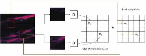
Adversarial loss is computed by the discriminator to improve the similarity between the distribution of $fak{e}_n$ and the distribution of $rea{l}_n$. The discriminator of the original GAN is designed to output only one value, the evaluation of the whole sample produced by the generator or the real input. In SinGAN, the model uses the PatchGAN discriminator, the output of which is no longer a single value, but a matrix. Each value in the matrix represents the evaluation of a small region, called a patch or receptive field, of the input (Knyaz et al., 2018). Compared to the original GAN, which uses one value for the evaluation, the PatchGAN discriminator evaluates the entire input through a matrix, allowing to focus on different regions of the input. By discriminating different patches separately, local features can be extracted, which is conducive to producing more realistic results. The discriminator’s final score is the average of the patch discrimination map, which is the matrix obtained by the PatchGAN discriminator (Jetchev et al., 2016). This type of adversarial loss is the key to achieving good results when SinGAN processes samples. By giving the same attention to different patches, the discriminator tries to distinguish the difference in each patch, while the generator tries to generate the true sample for each patch.

However, regarding climate data, more attention is often paid to extreme-value areas, as these may be associated with extreme events. For example, for precipitation data, extreme-value areas indicate the occurrence of floods. To enhance the simulation performance of the model for extreme-value regions based on SinGAN, we add a patch weight map according to apatch discrimination map. Instead of using the average of the patch discrimination map as the final score, we use the weighted average as the final output of the discriminator. The weight corresponding to each value in the patch discrimination map is determined by the ratio of the average value of the corresponding patch in the original real input to the sum of the averages of all patches. Figure 3 shows the structure of the weighted patchGAN discriminator. We assume there are $k$ patches in the original real input, and the average value of each patch is $\left\{p_1,p_2,...,p_{k-1},p_k\right\}$. Then, the final output of WSinGAN discriminator ($D_{out}$) is calculated as follows:

$W_i=\frac{p_i}{{\sum }_{j=1}^{j=k}{p}_j}$

$D_{out}\hspace{0.17em}={\sum }_{j=1}^{j=k}{D}_j\ast W_j.$

Figure 3. Structure of the weighted patchGAN discriminator.

3. Experimental setup

3.1. Datasets for training and testing

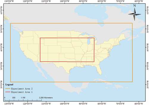
The Global Precipitation Measurement (GPM) is an international network of satellites collaboration with the National Aeronautics and Space Administration (NASA) and the Japan Aerospace Exploration Agency (JAXA) that will provide the next generation of global observations of precipitation and snow (Levizzani et al., 2007; Skofronick-Jackson et al., 2017). GPM can provide precipitation data with a maximum resolution of 0.1 degrees. To verify the performance of the modified SinGAN when generating HR climate data, we used GPM precipitation data from NASA with a raw spatial resolution of 0.1°×0.1° as the experimental subject. GPM precipitation data have different versions, and in this study, we used GPM_3IMERGDF, which is daily precipitation data that combine microwave-IR estimates with gauge calibration. Because a ground truth is required when evaluating different models, we regard the raw resolution of GPM precipitation data as both HR data and ground truth. Meanwhile, we downsampled the raw GPM data by a factor of 4, with an average sample pooling of 4 × 4 raster, and the coarsened 0.4°×0.4° resolution data was used as the LR input for all experiments with the aim of increasing the resolution of the input by a factor of 4. The data from area 1 (longitude: −113.199° to −84.100° and latitude: 32.300° to 46.099°) in Figure 4 were used to compare the results of different models (Section 4.1) and to check the temporal scalability of WSinGAN (Section 4.2.1), and area 2 (longitude: −129.199 to −63.805 degrees and latitude: 21.302° to 56.099°) was used to verify the spatial scalability of WSinGAN (Section 4.2.2). Daily precipitation data for the period 2019 to 2020, with 731 samples in total, were used as test data for the experiments. We compared the results of WSinGAN with four other models, among which WSinGAN, SinGAN, and bilinear and cubic interpolation did not require additional training data. These models were applied to each time step of the data individually to obtain the corresponding HR data. For the SRCNN, we first trained the network with corresponding pairs of LR and HR data. Daily precipitation data from June 1, 2000, to December 31, 2018 were used to train the model, and the SRCNN performance was tested using the same test data. A monthly precipitation dataset provided by the GFDL-ESM4 model from the Coupled Model Intercomparison Project (CMIP6) was collected to verify the results of the proposed model when applied to the GCM data (Dunne et al., 2020). We used monthly precipitation starting from January 2022 to January 2023 with a spatial resolution of 1° latitude × 1.25° longitude under the scenario of SSP1–2.6. To minimize the distortion near the poles, we only used data from latitudes undefined°.

Figure 4. Experimental areas (Experimental area 1 for Section 4.1 and Section 4.2.1; Experimental area 2 for Section 4.2.2).

3.2. Model configuration

All networks were implemented using a GPU (Tesla V100-SXM2-16GB on Google Colab). During the process of training SinGAN/WSinGAN, each layer of the GAN was trained separately and in the order of low to high. Each GAN layer was iterated 2,000 times, with an initial learning rate of 0.0005 and decays at a rate of 1/10 after 1,600 iterations. After each GAN layer was trained, the weights associated with it were fixed. Adaptive Moment Estimation was used to optimize the generator and discriminator, while the learning rate was set to 0.0005, and batch normalization (BN) was used to reduce overfitting during the training process. The negative slope of LeakyReLU was 0.2.

3.3. Evaluation metrics

We used the root mean squared error (RMSE) and Pearson’s correlation to evaluate the applicability of WSinGAN, as well as the overall model performance. The false alarm ratio (FAR; Ahmed et al., 2013) and threat score (TS) are commonly used in climate data evaluations to evaluate the effect of the model on the generation of extreme event regions, and they are calculated as follows:

$FAR=\frac{NB}{NA+NB}$

$TS=\frac{NA}{NA+NB+NC}.$

When calculating FAR, $NA$ is the number of grids when the result of the model has precipitation similar to the target. $NB$ denotes the number of grids when the result of the model has precipitation, though not within the target. When calculating TS, we must set a threshold value and: if the value of the grid is greater than or equal to the threshold, we assume the grid detects the event, and if the value of the grid is less than the threshold, we assume the grid misses the event. $NA$ represents the number of grids where the result of the model is the same as the target. $NB$ denotes the number of grids where the result of the model detects the event but the target misses it. $NC$ denotes the number of grids where the result of the model has no event but the target does. To test the model’s simulation results for extreme-value areas, we set three thresholds: 50th percentile, 75th percentile, and 95th percentile of daily precipitation.

4. Results

4.1. Comparing results of WSinGAN with those of other models

In this section, we compare the performance of WSinGAN with the original SinGAN, SRCNN, and bilinear and cubic interpolation. All results are from the test data in the study area, and our goal is to increase the resolution of LR data by a factor of 4. Table 1 shows a comparison of the different models, and all the results are calculated at each location of one sample and then averaged across the years 2019 to 2020 (test set). It can be seen that WSinGAN significantly outperforms the other four models in terms of all four metrics. For the RMSE, the three deep learning methods are better than bicubic and bilinear interpolation, while SRCNN and SinGAN are remarkably close to them. WSinGAN’s correlation coefficient is the only one that reached 0.90, while the other four models reached around 0.8. The RMSE and correlation can be used to evaluate the overall performance of the results, and we can conclude that adding the weighted patchGAN discriminator improved the overall quality of the generated HR climate data. For FAR, WSinGAN value is 0.09, while the other models’ values exceed 0.10. Its lowest FAR value means that the HR precipitation results generated by WSinGAN rarely show events that did not actually occur. The TS values have a decreasing trend for all five models as the thresholds increase, which demonstrates the challenge of generating these regions with extreme events when generating HR precipitation data. The two interpolation methods are slightly better than the three deep learning models when the threshold of TS is the 50th percentile. However, WSinGAN outperforms the interpolation methods when the threshold of TS is the 75th and 95th percentiles. The trend of TS indicates that WSinGAN has an excellent performance in the area of extreme events.

Table 1. Comparison of ability to generate HR data between five models.

Model	RMSE (mm/day)	Correlation	FAR	TS
				50th	75th	95th
SRCNN	2.28	0.82	0.12	0.76	0.58	0.56
Bilinear interpolation	2.38	0.83	0.11	0.81	0.68	0.52
Cubic interpolation	2.31	0.82	0.10	0.82	0.67	0.52
SinGAN	2.25	0.79	0.12	0.70	0.51	0.43
WSinGAN	1.80	0.90	0.09	0.79	0.71	0.65

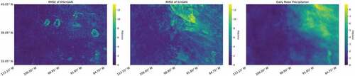
As previously stated, downscaling averages and extreme events in one single approach is challenging. Different quantitative thresholds are used to test the ability of each method to capture extreme events. At each grid in our research area, all precipitation values above the percentile threshold were selected first, and then the RMSE and correlation were calculated based on the selected data. This step was performed in a range of percentages between 75 and 99.9, and the result was averaged over all locations and all samples. As can be seen from Figure 5, for both the RMSE and correlation, although both became worse as the percentile increased, WSinGAN consistently outperformed the other four models, and this advantage is stable. Similar results are shown in Figure 6, where we calculated the distribution of the RMSE for SinGAN and WSinGAN at different locations. The plot on the right shows the average daily rainfall at each location, where we can see that the precipitation in the top right of the study area is greater than that in other areas. When comparing the RMSE distributions of SinGAN and WSinGAN, we find that for WSinGAN, only a minuscule area appears yellow, while a larger yellow area appears in SinGAN results, implying a larger RMSE. The regions with larger RMSEs in SinGAN results mainly appear to have some overlap with the regions with average precipitation. Using SinGAN’s discriminator, HR data are divided into patches, and the discriminator then determines the probability that each patch is true. The final discriminator score is the average over the probabilities of each patch. According to climate data, some areas tend toward extreme climate events, while others tend toward more stable events (in our example, most regions have zero rainfall). The contribution of the errors in these regions that have experienced extreme climatic events to the final loss will be reduced if the probabilities of these patches are averaged. In WSinGAN, rather than averaging the probabilities for these patches, we use a weighted average, where there is a greater contribution to the final loss if the region has a higher average precipitation. Figure 6 illustrates further that by adding the weighted patchGAN discriminator, not only is the overall performance promising when generating HR precipitation data, but a smaller error in extreme-value regions is also obtained.

Figure 5. Comparison of different models for the increasingly extreme precipitation. Left: RMSE; right: Correlation.

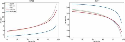
Figure 6. Comparison of the average RMSE computed at each location from WSinGAN and SinGAN across the test data. Left: WSinGAN. Middle: SinGAN. Right: Daily mean precipitation calculated across the test data.

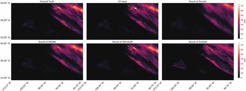
Figure 7 shows the HR results from cubic interpolation, SinGAN, and WSinGAN. Compared with the ground truth, we can see that WSinGAN result is physically more realistic than the results of bicubic interpolation and SinGAN, exhibiting refined small-scale features in areas of extreme event values and sharp gradients. SinGAN is also good at depicting sharp gradients, but it underestimates the extreme-value regions on the top right. Cubic interpolation, while recovering the extreme-value regions in the HR rainfall data, produces a relatively smoother result. Qualitatively, the results of WSinGAN are most comparable with the ground truth.

Figure 7. Comparison of various models on sample with time label: 20191030.

4.2. Analysis of scalability of pre-trained WSinGAN

The advantage of WSinGAN (and SinGAN) is that it does not require extra training data, and the corresponding HR data can be generated by training based on one single sample. When using SinGAN for natural images, each image must be trained separately, as different images have different intrinsic distributions, meaning the relationship between the LR and HR of natural images is not the same for different images. However, the internal distribution of the climatological precipitation data of a specific region may not vary significantly within a certain period. If different samples contain the same internal relationship between LR and HR data, then a pre-trained WSinGAN based on one sample may be applicable to other unseen samples. We discuss the result of testing the scalability of a pre-trained WSinGAN in this section.

4.2.1. Temporal scalability of WSinGAN

Because daily precipitation data are used in this study, temporal scalability is defined here as the applicability of WSinGAN to unseen data when the model is trained using precipitation data from a particular day. In Section 4.1, we obtained 731 pre-trained WSinGANs in total, corresponding to the size of the test data. We randomly selected 100 pre-trained WSinGANs from them, and then applied these 100 pre-trained WSinGANs to the test data separately. For each pre-trained WSinGAN, 731 HR precipitation data points were generated and then compared with the ground truth of the test data. Table 2 shows the metrics for the results of these 100 models. The mean RMSE for the pre-trained model is 2.38, with a standard deviation of 0.77, and despite being worse than the result of WSinGAN in Section 4.1, where each sample in the test set is trained separately, this result is still comparable to the other four models. Concerning FAR and TS, the mean values of the pre-trained models are 0.10 and 0.61, respectively; despite also being worse than the mean values of WSinGAN discussed in Section 4.1, they outperform those of the other four models. These measurements show that although the procedure for training WSinGAN is based on a single sample, it still has good temporal scalability for other data with unseen data

Table 2. Performance using pre-trained model on test data.

Model	RMSE (mm/day)	FAR	TS 95th
Mean value of 100 Pre-trained WSinGANs	2.38$\pm$0.77	0.10$\pm$0.06	0.61$\pm$0.07

To investigate this problem in depth, we counted the RMSE values generated by each pre-trained model applied to each test sample. Figure 8 shows the distribution of RMSE and the maximum values and standard deviations of the samples corresponding to the 100 pre-trained models in the training process. The top panel of Figure 8 shows a similar conclusion to Table 2, which is that the pre-trained model obtains small RMSE values for most of the test samples. However, we can still find some pre-trained models with worse results, such as models 5, 64, and 87. When we explore the relationship between the performance of the pre-trained model and the data used in the model training process, we find that the pre-trained models with larger RMSE values tend to be trained by samples with smaller maximum values and standard deviations, such as models 70, 5, and 90. Considering that much of the daily precipitation data have a minimum value of 0, a larger maximum value implies that the sample contains a wider range of rainfall magnitudes, and a larger standard deviation suggests a more heterogeneous distribution of precipitation in the sample. Such samples can provide richer spatial distribution information in the training process and establish more complete relationships between LR and HR data, supporting the pre-trained model with stronger scalability. We can see similar conclusions in Figure 9, where the worse FAR and TS results are mainly found in the region of smaller maxima and standard deviations. As the maximum and standard deviations gradually increase, most of the pre-trained models maintain a good performance. Figure 10 visualizes the results of one sample, where the bottom panels show the results of two different pre-trained models. Compared to the ground truth, the extreme events region and some details contained in the samples are also captured by the pre-trained models.

Figure 8. RMSE of the simulation of the test set using the pre-trained model, together with the standard deviation and maximum value of the data corresponding to the process of training the pre-trained model (Top: RMSE for each pre-trained model corresponding to the test set; Bottom left: Standard deviation of the sample used in the pre-trained model; Bottom right: Max value of the sample used in the pre-trained model).

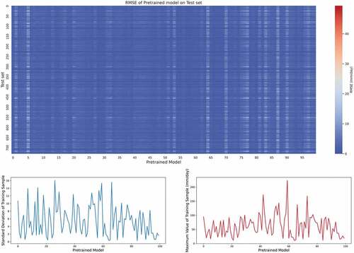
Figure 9. The standard deviation and maximum value of the sample used in the pre-trained model with respect to FAR and TS.

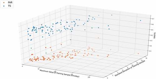
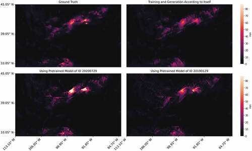
Figure 10. Result of using a pre-trained model for the unseen sample of ID 20,190,809. (Top left: Ground Truth; top right: Training and generation based on itself; bottom: using two pre-trained models).

4.2.2. Spatial scalability of WSinGAN

In this section, we examine the spatial scalability of WSinGAN. Notice that the generator network’s fully convolutional architecture allows it to be trained on relatively large areas, but it may be assessed on data fields of any size. The spatial scalability of the pre-trained model refers to its ability to generate HR precipitation data for smaller spatial scales using a pre-trained model that is trained based on data from a larger spatial scale. We selected 100 time points between 2019 and 2020 and obtained 100 pre-trained models by training WSinGAN using data from region 2, as mentioned in Section 3. For each time point, i.e. each pre-trained model, we randomly generated 10 smaller ranges in region 2 as test samples to generate HR precipitation data. In total, 1,000 results are summarized in Table 3. From the table, we can see that WSinGAN shows promising spatial scalability. Compared with the test result of temporal scalability, it has a smaller standard deviation, which means the spatial scalability of WSinGAN is more stable, predictable conclusion. As mentioned, previously, the process of training WSinGAN aims to learn the intrinsic statistics and distribution patterns within the sample. When training with a larger area of data, the information of small areas contained in it is also learned. From Figure 11, we can see that the results obtained using the pre-trained model are remarkably similar to the ground truth. The results for the extreme events region and the sharp gradient are also similar to those obtained using the corresponding sample for training.

Figure 11. Result of using a pre-trained model for the unseen sample of ID 20,190,809. (Top left: Ground Truth; top right: Training and generation based on itself; bottom: results using two different pre-trained models).

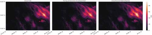
Table 3. Performance of using a pre-trained model with a large area on test data.

Model	RMSE (mm/day)	FAR	TS 95th
100 Pre-trained WSinGAN	2.18$\pm$0.20	0.10$\pm$0.02	0.63$\pm$0.03

4.3. Application to GCM climate data

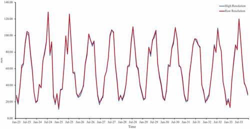
In this section, we discuss how we applied WSinGAN to the CMIP6 data. Because the raw CMIP6 data have a relatively LR, we selected a large range for our testing. The original raster size is 120 × 288 with a resolution of 1° × 1.25°; by increasing the resolution by a factor of four, we increased the size of the raster to 480 × 1152. Figure 12 shows the distribution of precipitation before and after the resolution improvement. As shown, the generated HR precipitation data preserve the original resolution while adding more details. WSinGAN generates the corresponding HR output based on the original CMIP6 data, so no ground truth HR data were available for evaluating our results. To illustrate the results of the model further, we calculated the average precipitation of the raw CMIP6 data and the generated HR data in the range of 25° N to 49° N, 70° W to 130° W, roughly covering the contiguous United States. The obtained time series are presented in Figure 13. Note that we only changed the spatial resolution of the CMIP6 data; its temporal resolution remains the same as the original data (monthly scale). There are 132 time points in the time series from January 2023 to January 2033, and the average RMSE of the generated HR rainfall data is 1.84 mm. As shown, WSinGAN maintains the average precipitation level of the original data while improving the resolution, both during summer months with higher precipitation levels and during winter months with lower precipitation levels.

Figure 12. Generated high-resolution (HR) precipitation data for the GFDL-ESM4 model.

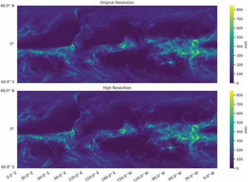
Figure 13. Comparison of average precipitation before and after downscaling in selected region (25° N to 49° N, 70° W to 130° W).

5. Discussion

In summary, these results show that WSinGAN is a powerful scientific tool to generate HR climatological precipitation data with a comparative performance for averages and extreme-value areas simultaneously. From the comparison of result 1, we can observe that WSinGAN outperforms the other four models with respect to all evaluation metrics. Instead of directly using the average of the patchGAN discriminator, we used the average of different patches in the original sample as the weights to calculate the final score. This modification improved WSinGAN results for extreme-value regions, as shown in Figure 6. Although the RMSE and correlation became worse as the percentile became more extreme, WSinGAN consistently outperformed the other four models, and this advantage was stable. Comparing the HR results generated by different models shows that WSinGAN generates more realistic structures with sharper gradients. This advantage is crucial for subsequent climate-related studies using HR precipitation data. One thing to note is that we can improve the SRCNN performance by increasing the size of the training data. CNNs are trained specifically to optimize the RMSE, and they have the potential to reduce the RMSE continuously as more data for training become available. However, considering that the training and generating WSinGAN rely only on a single LR sample and do not require additional LR – HR training pairs, WSinGAN shows a wide range of applications, especially in solving the problem of obtaining HR climate data in the absence of training data.

For natural images, the intrinsic statistical distribution varies greatly from image to image. However, for climate data of a particular region, different samples often have similar distribution characteristics. Because SinGAN can effectively capture and access the internal relationship of the input data, we check the scalability of the pre-trained WSinGAN, which relies on only one sample for training. The temporal and spatial scalability of the pre-trained WSinGAN are examined separately, and the results demonstrate that the pre-trained WSinGAN can generate good HR data for unseen data when WSinGAN is trained on one sample. The performance of the pre-trained WSinGAN is worse than that of training with the sample itself, but it is still comparable to the other four models. We also find that the performance of the pre-trained WSinGAN is related to the features of the sample used in the training process. Further, this pre-trained WSinGAN performs better when the training process uses a sample with a large maximum value and large standard deviation. A larger maximum value always implies that the sample contains a wider range of precipitation magnitudes, while a larger standard deviation suggests a more heterogeneous distribution of precipitation across the sample. Such a sample can provide richer spatial distribution information in the training process and establish more complete relationships from LR to HR data. We also examine the spatial scalability of the pre-trained WSinGAN. When WSinGAN is trained with a larger spatial region of data, the pre-trained WSinGAN is applicable to small areas within that region.

In this paper, we only tested WSinGAN with precipitation data. Much of the following work can be done to explore further the role of WSinGAN in generating HR climate data. Result 2 shows that the pre-trained WSinGAN has good temporal scalability. This offers the possibility that instead of training WSinGAN using one single sample, training with a limited number of representative samples may improve the simulation results of the model for unseen samples without adding extensive training time. Because precipitation in different seasons features different characteristics, we can focus on selecting representative samples to train the model in subsequent studies. In addition, the distribution of climate data is usually related to the topography. Adding the digital elevation model (DEM) to the training process has the potential to improve the performance of WSinGAN. Finally, the process of obtaining HR data from LR data has uncertainty, as the same LR pattern may correspond to multiple HR results. Generating HR data while considering the probability is highly informative for subsequent research, especially for disaster prediction, and additional experiments that examine higher multiplicities will be useful for WSinGAN applications.

6. Conclusion

Considering that the current deep learning models applied to obtain HR climate data are trained using LR and HR pairs, they are not effective when training data are insufficient. In this paper, we adapted SinGAN to generate HR climate data. Because SinGAN can rely on individual LR input data to obtain the corresponding HR result, it does not require large datasets for training. Instead of directly using the average value of the patchGAN discriminator, we used the average of different patches in the original sample as the weights to calculate the final score of the discriminator. The proposed WSinGAN outperforms the other models mentioned in the paper in generating HR precipitation data for both average areas and extreme-value areas. WSinGAN is most comparable to real HR data with sharp gradients and more refined small-scale features. We also tested the scalability of the pre-trained WSinGAN for unseen samples and show that although the training of WSinGAN relies only on a LR sample, it can still produce reliable HR data for unseen data. Thus, WSinGAN is a powerful tool for generating HR climate data when training data are insufficient.

Disclosure statement

No potential conflict of interest was reported by the author(s).

Data availability statement

Original GPM data can be downloaded from NASA at https://www.nasa.gov/mission_pages/GPM/main/index.html. CMIP6 data can be downloaded from https://cds.climate.copernicus.eu/cdsapp#!/home. The codes and datasets that support the findings of this study are available in 10.6084/m9.figshare.17203784.

Additional information

Notes on contributors

Yang Wang

Yang Wang is currently working toward the Ph.D. degree in Information Science in the School of computing and Information at the University of Pittsburgh. His research interests include spatio-temporal data mining, machine learning, climate dynamics, and geoinformatics. He received the M.S. degree in Civil Engineering from Swanson School of Engineering at the University of Pittsburgh. Before coming to the United States, he received the M.S. degree in Hydrology and Water Resources from Hohai University, Nanjing, China.

Hassan A. Karimi

Hassan A. Karimi is a Professor and the Director of the Geoinformatics Laboratory in the School of Computing and Information at the University of Pittsburgh. He obtained a BS in Computer Science from the University of New Brunswick and a MS in Computer Science and a PhD in Geomatics Engineering from the University of Calgary. Karimi’s research interests include computational geometry and topology, machine learning, spatial data analytics, navigation techniques and applications, location-based services, mobile computing, and distributed/parallel computing. His recent book is: Geospatial Data Science Techniques and Applications (lead editor), published by Taylor & Francis (2018).

References

- Ahmed, K. F., Wang, G., Silander, J., Wilson, A. M., Allen, J. M., Horton, R., & Anyah, R. (2013). Statistical downscaling and bias correction of climate model outputs for climate change impact assessment in the U.S. northeast. Global and Planetary Change, 100, 320–332. https://doi.org/10.1016/j.gloplacha.2012.11.003
- Bonan, G. B., & Doney, S. C. (2018). Climate, ecosystems, and planetary futures: The challenge to predict life in Earth system models. Science, 359(6375). https://doi.org/10.1126/science.aam8328
- Cheng, G., Zhang, F., & Qiang, X. (2020). Super-resolution reconstruction of rock thin-section image based on SinGAN. 2020 IEEE 9th Joint International Information Technology and Artificial Intelligence Conference (ITAIC), Chongqing, China (pp. 786–790).
- Chen, X.-W., & Lin, X. (2014). Big data deep learning: Challenges and perspectives. IEEE Access, 2, 514–525. https://doi.org/10.1109/ACCESS.2014.2325029
- Chen, S.-T., Yu, P.-S., & Tang, Y.-H. (2010). Statistical downscaling of daily precipitation using support vector machines and multivariate analysis. Journal of Hydrology, 385(1–4), 13–22. https://doi.org/10.1016/j.jhydrol.2010.01.021
- Dong, C., Loy, C. C., He, K., & Tang, X. (2015). Image super-resolution using deep convolutional networks. IEEE Transactions on Pattern Analysis and Machine Intelligence, 38(2), 295–307. https://doi.org/10.1109/TPAMI.2015.2439281
- Dunne, J. P., Horowitz, L. W., Adcroft, A. J., Ginoux, P., Held, I. M., John, J. G., Krasting, J. P., Malyshev, S., Naik, V., Paulot, F., & Shevliakova, E. (2020). The GFDL Earth System Model version 4.1 (GFDL‐ESM 4.1): Overall coupled model description and simulation characteristics. Journal of Advances in Modeling Earth Systems, 12(11), e2019MS002015. https://doi.org/10.1029/2019MS002015
- Frey-Buness, F., Heimann, D., & Sausen, R. (1995). A statistical-dynamical downscaling procedure for global climate simulations. Theoretical and Applied Climatology, 50(3), 117–131. https://doi.org/10.1007/BF00866111
- Gu, S., Zhang, R., Luo, H., Li, M., Feng, H., & Tang, X. (2021). Improved SinGAN integrated with an attentional mechanism for remote sensing image classification. Remote Sensing, 13(9), 1713. https://doi.org/10.3390/rs13091713
- Hutengs, C., & Vohland, M. (2016). Downscaling land surface temperatures at regional scales with random forest regression. Remote Sensing of Environment, 178, 127–141. https://doi.org/10.1016/j.rse.2016.03.006
- Huth, R. (2002). Statistical downscaling of daily temperature in central Europe. Journal of Climate, 15(13), 1731–1742. doi:10.1175/1520-0442(2002)015<1731:SDODTI>2.0.CO;2
- Ioffe, S., & Szegedy, C. (2015). Batch normalization: Accelerating deep network training by reducing internal covariate shift. International conference on machine learning, Lille, France, (pp. 448–456).
- Jetchev, N., Bergmann, U., & Vollgraf, R. (2016). Texture synthesis with spatial generative adversarial networks. arXiv preprint arXiv:1611.08207.
- Kim, J., Lee, J. K., & Lee, K. M. (2016). Accurate image super-resolution using very deep convolutional networks. Proceedings of the IEEE conference on computer vision and pattern recognition, Las Vegas, Nevada, USA, (pp. 1646–1654).
- Knyaz, V. A., Kniaz, V. V., & Remondino, F. (2018). Image-to-voxel model translation with conditional adversarial networks. Proceedings of the European Conference on Computer Vision (ECCV) Workshops, Munich, Germany.
- Ledig, C., Theis, L., & Husza ́r, F. (2017). Photo-realistic single image super-resolution using a generative adversarial network. Proceedings of the IEEE conference on computer vision and pattern recognition, Honolulu, Hawaii, USA, 4681–4690.
- Levizzani, V., Bauer, P., & Turk, F. J. (2007). Measuring precipitation from space: EURAINSAT and the future. Springer Science & Business Media.
- Rocha Rodrigues, E., Oliveira, Igor, Renato and Netto, Marco. (2018). DeepDownscale: A deep learning strategy for high-resolution weather forecast. 2018 IEEE 14th International Conference on e-Science (e-Science), Amsterdam, Netherlands, 415–422.
- Rockel, B., Castro, C. L., Pielke, R. A., von Storch, H., & Leoncini, G. (2008). Dynamical downscaling: Assessment of model system dependent retained and added variability for two different regional climate models. Journal of Geophysical Research: Atmospheres, 113(D21). https://doi.org/10.1029/2007JD009461
- Schiermeier, Q. (2010). The real holes in climate science. Nature News, 463(7279), 284–287. https://doi.org/10.1038/463284a
- Shaham, T. R., Dekel, T., Michaeli, T. . (2019). Learning a generative model from a single natural image. ed. Proceedings of the IEEE/CVF International Conference on Computer Vision, Seoul, South Korea (pp. 4570–4580).
- Skofronick-Jackson, G., Petersen, W. A., Berg, W., Kidd, C., Stocker, E. F., Kirschbaum, D. B., Kakar, R., Braun, S. A., Huffman, G. J., Iguchi, T., Kirstetter, P. E., Kummerow, C., Meneghini, R., Oki, R., Olson, W. S., Takayabu, Y. N., Furukawa, K., & Wilheit, T. (2017). The Global Precipitation Measurement (GPM) mission for science and society. Bulletin of the American Meteorological Society, 98(8), 1679–1695. https://doi.org/10.1175/BAMS-D-15-00306.1
- Stengel, K., Glaws, A., Hettinger, D., & King, R. N. (2020). Adversarial super-resolution of climatological wind and solar data. Proceedings of the National Academy of Sciences of the United States of America, 117(29), 16805–16815. https://doi.org/10.1073/pnas.1918964117
- Sun, W., & Liu, B.-D. (2020). ESinGAN: Enhanced single-image GAN using pixel attention mechanism for image super-resolution. 2020 15th IEEE International Conference on Signal Processing (ICSP), Beijing, China (pp. 181–186).
- Tank, A., Zwiers, F., & Zhang, Z. (2009). Guidelines on analysis of extremes in a changing climate in support of informed decisions for adaptation. World Meteorological Organization.
- Tian, J., Liu, J., Wang, Y., Wang, W., Li, C., & Hu, C. (2020). A coupled atmospheric–hydrologic modeling system with variable grid sizes for rainfall–runoff simulation in semi-humid and semi-arid watersheds: How does the coupling scale affects the results? Hydrology and Earth System Sciences, 24(8), 3933–3949. https://doi.org/10.5194/hess-24-3933-2020
- Vandal, T., Kodra, Evan, Ganguly, Sangram, Michaelis, Andrew, Nemani, Ramakrishna and Ganguly, Auroop R. (2017). Deepsd: Generating high resolution climate change projections through single image super-resolution. Proceedings of the 23rd acm sigkdd international conference on knowledge discovery and data mining, Halifax, NS, Canada, 1663–1672.
- Wamsler, C., Brink, E., & Rivera, C. (2013). Planning for climate change in urban areas: From theory to practice. Journal of Cleaner Production, 50, 68–81. https://doi.org/10.1016/j.jclepro.2012.12.008
- Wang, X., Yu, Ke. Wu, Shixiang, Gu, Jinjin. Liu, Yihao. Dong, Chao. Qiao, Yu and Change Loy Chen. (2018). Esrgan: Enhanced super-resolution generative adversarial networks. Proceedings of the European conference on computer vision (ECCV) workshops, Munich, Germany.
- Wilby, R. L., Wigley, T. M. L., Conway, D., Jones, P. D., Hewitson, B. C., Main, J., & Wilks, D. S. (1998). Statistical downscaling of general circulation model output: A comparison of methods. Water Resources Research, 34(11), 2995–3008. https://doi.org/10.1029/98WR02577
- Xinwei, L., Jinlin, Guo, Jinshen, Dou and Songyang, Lao (2021). Generating constrained multi-target scene images using conditional SinGAN. 2021 6th International Conference on Intelligent Computing and Signal Processing (ICSP), Xi'an, China, 557–561.
- Yang, Y., Cao, C., Pan, X., Li, X., & Zhu, X. (2017). Downscaling land surface temperature in an arid area by using multiple remote sensing indices with random forest regression. Remote Sensing, 9(8), 789. https://doi.org/10.3390/rs9080789
- Yang, W., Zhang, X., Tian, Y., Wang, W., Xue, J.-H., & Liao, Q. (2019). Deep learning for single image super-resolution: A brief review. IEEE Transactions on Multimedia, 21(12), 3106–3121. https://doi.org/10.1109/TMM.2019.2919431
- Zhang, B., Xu, G., Jiao, L., Liu, J., Dong, T., Li, Z., Liu, X., & Liu, Y. (2019). The scale effects of the spatial autocorrelation measurement: Aggregation level and spatial resolution. International Journal of Geographical Information Science, 33(5), 945–966. https://doi.org/10.1080/13658816.2018.1564316