The synergies of SMAP enhanced and MODIS products in a random forest regression for estimating 1 km soil moisture over Africa using Google Earth Engine

ABSTRACT

Due to the coarse scale of soil moisture products retrieved from passive microwave observations (SM_PMW), several downscaling methods have been developed to enable regional scale applications. However, it can be challenging for users to access final data products and algorithms, as well as managing different data sources and formats, various data processing methods, and the complexity of the workflows from raw data to information products. Here, the Google Earth Engine (GEE), which as of late offers SM_PMW, is used to implement a workflow for retrieving 1 km SM at a depth of 0–5 cm using MODIS optical/thermal measurements, the SM_PMW coarse scale product, and a random forest regression. The proposed method was implemented on the African continent to estimate weekly SM maps. The results of this study were evaluated against in-situ measurements of three validation networks. Overall, in comparison to the original SM_PMW product, which was limited by a spatial resolution of only 9 km, this method is able to estimate SM at 1 km spatial resolution with acceptable accuracy (an average correlation coefficient of 0.64 and a ubRMSD of 0.069 m³/m³). The results show that the proposed method in GEE provides a precise estimation of SM with a higher spatial resolution across the entire continent.

KEYWORDS:

• Soil moisture
• SMAP
• Google Earth Engine
• random forest regression
• MODIS

1. Introduction

Soil moisture (SM) plays a crucial role in hydrological, biological, and biogeochemical processes (Khazaei et al., 2023; Piou et al., 2019). It influences the water and energy cycle, affecting evaporation and transpiration (Adab et al., 2020; Vereecken et al., 2014). SM also impacts the response of the water cycle to changes and drainage into streams and rivers (Mohseni et al., 2021; Montzka et al., 2021; Seneviratne et al., 2006). Understanding SM improves weather prediction models and supports various studies such as floods, droughts, and climate events. Continuous SM datasets are essential for meteorology, energy cycles, and engineering (Babaeian et al., 2019; Mohseni & Mokhtarzade, 2021; Peng et al., 2021).

Remote Sensing (RS) techniques make it possible to observe SM at a global scale with sufficient time continuity, even in difficult and inaccessible locations (Brocca et al., 2023; Mohanty et al., 2017; Mohseni & Mokhtarzade, 2020). Various studies have demonstrated that passive microwave radiometers are one of the most efficient RS technologies for SM estimation, due to their high sensitivity to the soil dielectric constant, which has a direct relationship with SM (Xu et al., 2022). Since late 1970s, data from various RS microwave radiometers have been utilized to retrieve SM. Soil Moisture and Ocean Salinity (SMOS), in orbit since November 2, 2009 (Mecklenburg et al., 2012), and Soil Moisture Active Passive (SMAP), in orbit since January 31, 2015 (Montzka et al., 2016; Reichle et al., 2022), are the first two satellites dedicated to directly estimate near-real-time global SM. Both SMAP and SMOS suffer from the same shortcoming as the previous RS radiometers regarding their coarse-scale spatial resolution (approximately 9 km to 40 km), which is inadequate for studies at the regional or local level (Mohseni & Mokhtarzade, 2021; Mohseni et al., 2022).

Several efficient methods for retrieving SM with moderate and high spatial resolution have been developed to combine SM obtained from passive microwave observations (SM_PMW) with observations from other RS domains (such as optical, thermal, and active microwave) with higher spatial resolution (Peng et al., 2017). The underlying concept of these downscaling methods is that as SM influences emissivity, temperature dynamics, soil color, albedo, light absorption bands, and dielectric constant, a variety of SM-related indices can be calculated using different band ratios and band combinations of optical and thermal RS domains (Khellouk et al., 2020; Mohseni et al., 2021; Sahaar et al., 2022). Furthermore, active microwave backscattering signals of the land surface are also sensitive to SM (Mirmazloumi et al., 2021; Zribi et al., 2020). Both mentioned electromagnetic spectrum domains enable sensors to operate at higher spatial resolution than passive microwave, but SM retrieval is challenging without auxiliary data and more complex mathematical algorithms, considering, e.g., the complex spatio-temporal dynamics of vegetation cover (Pradhan et al., 2018). The use of these intermediate and high-resolution observations in combination with SM_PMW allows estimation of SM with higher spatial resolution (Petropoulos et al., 2015). The scaling methods can be categorized into various groups based on the features used to disaggregate the SM_PMW products: radar-based (Jagdhuber et al., 2019; Narayan & Lakshmi, 2008), radiometer based (de Jeu et al., 2014; Gevaert et al., 2016), optical/thermal-based (Chul Jung et al., 2019; Peng et al., 2017; Zheng et al., 2021a), data assimilation based (Fang et al., 2018; Lievens et al., 2015; Xu et al., 2020), and soil surface attributes-based methods (Montzka et al., 2018; Shin & Mohanty, 2013). Optical and thermal methods are widely used due to the extremely strong theoretical relationship between SM, surface temperature, and vegetation condition and easy access to data obtained from different optical/thermal satellites (Mohseni & Mokhtarzade, 2021).

So far, a vast number of empirical (Piles et al., 2016), physical-based (Merlin et al., 2005), data assimilation (Naz et al., 2020; Pellenq et al., 2003), and spatial interpolation methods (Kim & Barros, 2002) have been developed and applied to downscale SM_PMW using optical/thermal indices (Merlin et al., 2010; Sabaghy et al., 2018). Piles et al. (2011), applied a Linear Regression (LR) model to downscale SMOS data using Land Surface Temperature (LST), and Normalized Difference Vegetation Index (NDVI) of MODIS. Song et al. (2013) used a single-channel technique to downscale the BT observed by AMSR-E using an LR between Microwave Polarization Difference Index (MPDI) and NDVI. They retrieved SM from downscaled BT using a Single-Channel Algorithm (SCA). Similarity, Sánchez-Ruiz et al. (2014) used Normalized Difference Water Index (NDWI) calculated with three various MODIS Short Wave Infrared (SWIR) bands along with NDVI and LST to downscale SMOS data over the REMEDHUS network in Spain. Fang et al. (2022) and Hu et al. (2020) applied the Geographically Weighted Regression (GWR) method to obtain an optimal local regression for downscaling SMAP data using 8-day LST, and 16-day NDVI. Merlin et al. (2008) introduced a novel downscaling approach called Disaggregation based on Physical And Theoretical scale Change (DisPATCh) to disaggregate coarse-scale SM data based on a semi-empirical Soil Evaporative Efficiency (SEE) model and a first-order Taylor series expansion. A vast number of researches investigated the performance of DisPATCh over different study areas (Djamai et al., 2016; Fontanet et al., 2018; Malbéteau et al., 2016; Merlin et al., 2008; Montzka et al., 2018; Neuhauser et al., 2019; Qu et al., 2021; Zheng et al., 2021b).

Aside from the aforementioned empirical and semi-empirical methods, a number of studies have demonstrated the ability of Machine Learning (ML) models in downscaling SM_PMW (Zhao et al., 2021). Srivastava et al. (2013) compared the performance of the Generalized Linear Model (GLM) and three ML techniques including Artificial Neural Network (ANN), Support Vector Machine (SVM), and Relevance Vector Machine (RVM) to downscale SMOS products using MODLS LST. Abbaszadeh et al. (2019) presented 12 distinct Random Forest (RF) models to downscale the daily composite version of SMAP data using LST and NDVI data of MODIS along with soil texture and topography information of the study area. In this way, Hu et al. (2020) used LST, NDVI, horizontally and vertically polarized BT, and SWIR reflectance as the input data of the RF method to downscale SMAP products over Inner Mongolia. Bai et al. (2019) also applied RF to downscale SMAP product using the LST, NDVI, Enhanced Vegetation Index (EVI), NDWI, Leaf Area Index (LAI) derived from MODIS, backscattering coefficients of Sentinel-1, and surface elevation and slope as auxiliary data. Because downscaling methods are usually pixel-based and ignore the information among the neighbors of the pixels, Xu et al. (2021) proposed a new downscaling method based on a Convolutional Neural Network (CNN) and map-to-pixel approach during the network construction. In a study conducted by Ghafari et al. (2020), SMAP radiometer BT was downscaled to 3 km using airborne SAR backscatter observations collected during the fifth SMAP Experiment (SMAPEx-5) conducted in southeastern Australia. The study compared the results of these downscaled data with SMAP/Sentinel-1 SM data, which also had a spatial resolution of 3 km. Xu et al. (2022) proposed an SM downscaling framework based on the Wide & Deep Learning (WDL) method to improve the spatial resolution of SMAP product, using the horizontally and vertically polarized BT, LST, and surface reflectance. They also used topographic attributes, soil properties, climate types, and land cover types as auxiliary datasets to improve the accuracy of the WDL method.

Downscaling methods, whether using classical regression methods or machine learning, rely on the relationship between vegetation conditions, surface temperature, and SM. However, these methods present challenges. Firstly, they require multiple data sources with different formats and software for processing. Secondly, filling missing values, especially for cloudy conditions, is necessary. Thirdly, adjusting temporal resolutions and overpass times of the data sets is crucial. Lastly, limited accessibility and modification options for algorithms pose difficulties for non-experts seeking local-scale SM information (Khazaei et al., 2023).

The use of cloud computing platforms like Google Earth Engine (GEE) overcomes these challenges by providing access to extensive datasets from satellites, RS products, and model-based measurements (Mutanga & Kumar, 2019). GEE offers accessibility to diverse datasets, ready-to-use image-driven products, easy data upload, a wide range of image processing algorithms, and various computing techniques (Amani et al., 2020; Ghorbanian et al., 2020; Tamiminia et al., 2020). Multiple SMAP products, including SMAP L3 Radiometer Global Daily 9 km Soil Moisture and SMAP L4 Global 3-hourly 9-km Surface and Root Zone Soil Moisture, are available through GEE. These products provide global land surface conditions, SM measurements, meteorological variables, and other relevant data (Chan et al., 2016; Chen et al., 2018; Colliander et al., 2017; Kim et al., 2018; Ma et al., 2019). The SMAP mission outperforms earlier satellites in terms of resolution and accuracy. By leveraging GEE and statistical methods, merging coarse-scale SM_PMW data with other RS observations enables accurate high-resolution SM estimation.

The purpose of this study is to implement an optical/thermal-based downscaling procedure for estimating SM at 1 km spatial resolution at a depth of 0–5 cm using GEE for the African continent. The estimation of SM in Africa holds immense importance due to the consistent predictions of climate change models, indicating an increased occurrence of droughts and floods in various regions (Myeni et al., 2019). These climate change consequences pose a significant threat to the food security and livelihoods of smallholder farmers across the continent. SM plays a crucial role as a water source for plant growth between rainfall events, directly impacting crop yields and agricultural drought (Anderson et al., 2012). Therefore, accurate quantification of SM becomes a vital parameter in assessing weather-induced risks associated with climate change in Africa. Efforts have been made in recent years to establish in-situ SM monitoring networks, supporting satellite-based SM retrievals (McNally et al., 2016). Despite these advancements, there remains a persistent lack of comprehensive SM information in Africa, characterized by insufficient spatial resolution and acceptable accuracy. Consequently, further research and improvements are necessary to obtain SM data that adequately addresses the unique requirements and challenges faced in Africa.

By delving into the details, the novelty of this study can be analyzed from two distinct perspectives: Firstly, the study introduces a pioneering application of GEE for implementing a downscaling method, thereby surmounting the challenges associated with traditional downscaling approaches. Secondly, this study endeavors to estimate soil moisture SM at moderate resolutions for the entire continent of Africa, a task that has not been previously undertaken. Through the proposed methodology, it becomes feasible to consistently apply this approach across the entire continent, resulting in the generation of SM maps at a remarkable 1-km resolution, obviating the need for auxiliary data.

The proposed method in this study leverages the power of the GEE computing platform and generates a weekly SM in Africa. Similar to other downscaling methods, the proposed method has three main steps: (1) estimating SM-related features at moderate spatial resolution, (2) establishing a linking model between measured features and SM_PMW, and (3) estimating the SM at the spatial resolution of SM-related features. The proposed method employs RF Regression (RFR), known as one of the most effective ML techniques for establishing regression models between non-relative values (Mirmazloumi et al., 2022). The trained RFR model is subsequently applied to optical and thermal data to estimate SM at higher spatial resolutions. The strength of this methodology lies in its accessibility and user-friendliness, enabling researchers and scientists to work with the data and derive meaningful insights without requiring specialized software or technical expertise. Additionally, this approach offers the advantage of generating up-to-date data on demand.

The study area and satellite data used in this study are detailed in the next section. In Section 3, the proposed method, the RFR, and the SM indices are described. Results and discussion are presented in Section 4 and Section 5, respectively. In Section 6, the conclusion is presented.

2. Study area and data

In order to evaluate the effectiveness of the GEE to apply the SM_PMW downscaling algorithm, Africa (between 18°W and 25°E and 4°N and 18°N) is considered as the core study area. Given the variety of climatological, biogeographical, pedological, and lithological properties over the African continent (Zribi et al., 2008), different facets of the performance of the downscaling approach in GEE can be assessed in this area.

Over the last few years, several temporary or permanent SM validation networks with in-situ stations have been installed in Africa to support satellite retrievals, satellite product improvements, and assessments (Myeni et al., 2019). Some of these validation sites are listed in the International Soil Moisture Network (ISMN) to support the further validation of RS products at the global scale (Dorigo et al., 2021). AMMA-CATCH, DAHRA, SD_DEM, TAHMO, are four important SM measuring networks located in different parts of Africa. In addition, the Cosmic-ray Soil Moisture Observing System (COSMOS) has launched 14 validation stations in Africa. The networks measure the SM at various soil depths, ranging from 0–5 cm to 2 m depths every hour. Cosmic-ray Neutron Probes, TERSOS, and HYDRA are some of the detectors utilized at different stations to measure SM in Africa. These stations are found in different types of landscape, including wetlands, watersheds, urban areas, and croplands. Since TAHMO has the greatest number of stations (70 stations), it is important to consider the time period availability of this network. Given this prerequisite and the availability of other sites’ data, the largest time frame for which the maximum number of in-situ measurements is accessible and can be used for the validation process is the year 2020. For this time period, data from stations that measure SM up to 10 cm depth of the soil are gathered for the validation procedure. To ensure the reliability of our validation process, we have excluded in-situ data near water bodies and urban areas. This decision was made due to potential uncertainties introduced by the presence of these features, such as water bodies in wetlands, rivers, lakes, and the urban environment. By excluding such data points, we aim to minimize the impact of these sources on the accuracy of our SM measurements derived from passive microwave observations. Thirty-five stations from three different networks are remaining after the reference data analysis; their main characteristics are listed in Table 1, and their locations are displayed in Figure 1.

Figure 1. MODIS land cover map over the study area. In total, the 0–10 cm depth SM observations of 31 TAHMO stations, 1 COSMOS station, and 1 SD_DEM station are used in this study to validate the proposed method.

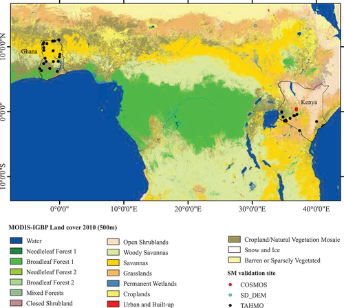
Table 1. The primary attributes of the SM sites which were used in the validation process.

Site	Number of stations	Land cover	Climate regime	Depth (m)	Detector	Reference
SD_DEM^1	1	Cropland	Dry\Desert	0.05, 0.10	CS615, HYDRA, CS616	(Ardö, 2013)
COSMOS^2	2	Cropland	Temperate	0.00–0.10	Cosmic-ray Probe	(Zreda et al., 2012)
TAHMO^3	32	Cropland, Grassland, Sparse vegetation, Bare area	Tropical, Temperate	0.10	TEROS12, GS1 TEROS10	(van de Giesen et al., 2014)

¹Soil Data_DEMokeya.

²Cosmic-ray Soil Moisture Observing System.

³Trans-African Hydro-Meteorological Observatory (name of in situ network in Sahel Zone in Africa).

Based on Table 1, most of the stations are located in croplands and have tropical and temperate regimes. For each station, the SM measurements at the depth of 0–10 cm between 6 am and 6 pm are averaged for each week and applied as ground reference data in the validation process.

2.1. Satellite data

Table 2 summarizes all satellite-based data applied in this study to estimate SM values at moderate spatial resolution. All of the data in Table 2 are available for download, processing, and use in GEE cloud computing platform (https://developers.google.com/earth-engine/datasets). A brief description of the main data pre-processing in this study is provided in Section 3.

Table 2. Main characteristics of the RS observations and products used in the downscaling methods.

Dataset	Data Type and Description	Spatial Resolution	Units	Revisit Time	Temporal Coverage
SPL4SMGP.007	SMAP L4 Global Surface and Root Zone Soil Moisture	9 km × 9 km	Volume fraction	3-hourly	2015-04-02 to present
MODIS/V006/MOD11A2	Daytime and nighttime land surface temperature (LST)	1 km × 1 km	Kelvin	8-day	2000-02-18 to present
MODIS/006/MOD09A1 Surface spectral reflectance	Band 05: Shortwave/NIR, 1230–1250 nm	500 m × 500 m	Unitless		2000-02-18 to present
	Band 06: Shortwave Infrared/SWIR, 1628–1652 nm
	Band 07: Shortwave Infrared/SWIR, 2105–2155 nm
MODIS/061/MOD13A1	Vegetation Index (NDVI)			16-day
MODIS/061/MCD12Q1	Land Cover Type	500 m × 500 m		Yearly	2001-01-01 to present

Based on the information provided in Table 2, this method utilizes various MODIS and SMAP data with different spatial and temporal characteristics. For land surface temperature (LST) observations, version 6 of the 8-day Terra LST and Emissivity product with a 1 km spatial resolution (MODIS/V006/MOD11A2) was used. Regarding reflectance in various NIR and SWIR bands and a vegetation index, this study employed the Terra surface spectral reflectance product (MODIS/006/MOD09A1) and vegetation fraction product (MODIS/061/MOD13A1), both at 500 m spatial resolution. Moreover, the global and yearly land cover type map of MODIS (MODIS/061/MCD12Q1) was also used.

The proposed method is implemented using SPL4SMGP.007 SM product available in GEE. SPL4SMGP.007 represents the level 4 of the SMAP product. This product merges SMAP observations into a physically based numerical land surface model simulating the water, energy, and carbon cycles. As a result, the level-4 data provides a global estimate of surface and root zone SM, surface and soil temperature, and land surface fluxes. Additionally, the product includes algorithm diagnostics derived from the ensemble-based data assimilation system (Entekhabi et al., 2014). SPL4SMGP.007 utilizes the SMAP radiometer data spatially enhanced to 9 km, based on the Backus–Gilbert optimal interpolation technique. This product is provided on the global cylindrical EASE-Grid 2.0 (Mohseni et al., 2022). For this study, data from January to December 2020 were averaged for each week before being used for downscaling SM.

3. Methodology

Figure 2 shows the proposed process of estimating SM at the local spatial resolution using GEE.

Figure 2. The workflow of the proposed method for estimating SM using GEE.

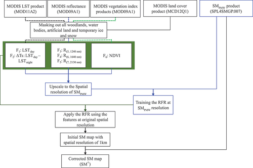
The underlying concept behind the proposed method is the relationship between SM, atmospheric condition, surface temperature, and vegetation. This approach is also known as the Universal Triangle Technique (UTT) or the Temperature-Vegetation (T-V) method (Carlson & Petropoulos, 2019). The theory states that for a given region, under particular climatic conditions, there is a unique relationship between SM, vegetation fraction (Fv), and surface temperature (Ts) (Carlson, 2007; Nichols, 2011). In general, SM is directly influenced by soil evaporation and vegetation transpiration, both of which influence the Ts observed by RS. It means that due to the cooling of the plant canopy by vegetation transpiration, the observed Ts decreases. Without water available to transpire, the canopy heats up. Denser vegetation is better able to cool its canopy than sparse vegetation. It can be said that there is a negative relationship between the observed Ts and Fv. However, the rate of the mentioned relationship between Ts and Fv is not equal in different SM and increases in the dry soil conditions (Mohseni & Mokhtarzade, 2020). Through the corresponding relationship, SM values can be estimated from Ts and Fv, both of which are measurable using RS observations. So far, a wide range of SM-related indices have been developed and calculated using optical/thermal RS products. As part of the application of the UTT, SM_PMW products and optical/thermal data have also been merged under the disaggregation method (Carlson & Petropoulos, 2019; Piles et al., 2010, 2011; Xu et al., 2018). There are three main steps in the downscaling method using optical/thermal observations: (1) estimating optical/thermal SM-related features at moderate spatial resolution, (2) establishing a linking model between optical/thermal features and SM_PMW, and (3) estimating the SM at the spatial resolution of MODIS product.

3.1. The estimation of optical/thermal SM-related features at moderate spatial resolution

In order to extract SM-related features from optical/thermal data, it is necessary to exclude all products and pixels that contain incorrect or inaccurate data from the input provided to the algorithm. For this purpose, any MODIS products with more than 20% of cloudy pixels were removed. Thermal features derived from MODIS observations may have some untraceable errors in estimation LST in woodlands and forests due to the limited penetration depth of optical and thermal bands within canopied areas. The accuracy of these features is a crucial factor that can impact the precision of the RFR model. The potential impact of woodland area on estimating SM-related features and then the performance of the RFR necessitates their exclusion from our proposed method. Subsequently, the flag data were processed by utilizing the MODIS LULC product to eliminate pixels corresponding to water bodies, artificial land, and temporary snow and ice. This step was also performed for the coarse-scale SM_PMW. Consequently, any pixels that consisted of more than 20% of water bodies, artificial land, temporary snow, or ice were excluded from the further processing. Additionally, all MODIS products were rescaled to a resolution of 1 km before being integrated into the downscaling workflow. This rescaling process was conducted in GEE by calculating the average values within 500 m and generating pixels with a spatial resolution of 1 km.

After removing pixels with weak data, SM-related features were extracted for the remaining pixels. In this study, and given the UTT method, NDVI product is used as the vegetation index. Moreover, the MODIS LST at the daytime (LST_day) and LST difference between daytime and nighttime ($\mathrm{\Delta }{\mathrm{T}}_s$, Eq. (1)) are applied as the temperature features. The $\mathrm{\Delta }{\mathrm{T}}_s$ is estimated using the observations of ascending and descending overpass time of MODIS.

(1) $\mathrm{\Delta }{\mathrm{T}}_s=\mathrm{LS}{\mathrm{T}}_{\mathit{day}}-\mathrm{LS}{\mathrm{T}}_{\mathit{night}}$(1)

Applying $\mathrm{\Delta }{\mathrm{T}}_s$ is based on Thermal Inertia Theory (TIT), which states that in the same environmental temperature variation, materials with low water content and, thereby, low heat capacity and thermal inertia, have a greater surface temperature difference (Fang et al., 2013). Moreover, the reflectance at three different NIR/SWIR bands, as the water absorption bands, including bands 5–7 of MODIS are also used in this study. The consideration of these three water absorption bands is grounded in previous studies that utilized NDWI or other indices derived from these specific bands to downscale SM_PMW data (Abbaszadeh et al., 2019; Sánchez-Ruiz et al., 2014). As the reflectance of the water absorption bands is influenced by SM, they hold significant potential as robust features for estimating SM in relation to soil characteristics.

All daily features and RS-products at both 9 km and 1 km spatial resolutions are then aggregated to produce weekly maps. It should be noted that several studies have attempted to predict shorter-term SM-related features, such as daily LST, daily evapotranspiration, etc., by employing different interpolation methods to estimate SM values at higher temporal resolutions (Han et al., 2010; Jung et al., 2017; Wang et al., 2011). However, the objective of using weekly inputs is to mitigate the impact of the accuracy of interpolation techniques in GEE performance and the outputs of downscaling workflow.

3.2. The establishment of a linking model between optical/thermal features and SM_PMW

In the second step of the proposed method, the relationship between SM and SM-related features extracted from RS data must be established (Eq. (2)) (Peng et al., 2017). This relationship can range from linear regression to various ML regression models (Sabaghy et al., 2018). Based on the UTT and TIT theory explained above, the following relationship can be established at the spatial resolution of SMAP:

(2) $\mathit{S}{M}_{\mathit{PMW}}=\mathit{f}\left(\mathrm{LS}{\mathrm{T}}_{\mathit{day}},\mathrm{\Delta }{\mathrm{T}}_s,\mathit{\hspace{0.17em}}{R}_{5\left(1240\mathit{nm}\right)},\mathit{\hspace{0.17em}}{R}_{6\left(1640\mathit{nm}\right)},\mathit{\hspace{0.17em}}{R}_{7\left(2130\mathit{nm}\right)},\mathrm{NDVI}\right)$(2)

The spatial resolution of SM_PMW in GEE is 9 km, which allows the estimation of the linking function (f, Eq. (2)(2) $\mathit{S}{M}_{\mathit{PMW}}=\mathit{f}\left(\mathrm{LS}{\mathrm{T}}_{\mathit{day}},\mathrm{\Delta }{\mathrm{T}}_s,\mathit{\hspace{0.17em}}{R}_{5\left(1240\mathit{nm}\right)},\mathit{\hspace{0.17em}}{R}_{6\left(1640\mathit{nm}\right)},\mathit{\hspace{0.17em}}{R}_{7\left(2130\mathit{nm}\right)},\mathrm{NDVI}\right)$(2) ) at this resolution. GEE has a number of built-in ML tools that are designed to work with multi-band raster data. In this study, we employed RFR designed in GEE as the linking function between optical/thermal features and SM_PMW observations. RFR is an ML algorithm specifically designed for regression problems. It utilizes an ensemble of decision trees to make predictions. In the RFR algorithm, numerous decision trees are created, each making predictions based on a subset of the data features. These individual predictions are then combined to generate a final prediction. This approach helps mitigate the risk of overfitting and enhances the accuracy of the predictions. RFR is commonly utilized in scenarios involving multiple predictors or features that may contribute to the outcome. Its ability to handle non-linear relationships and overfitting, achieved through the averaging of multiple decision trees, makes it valuable for establishing the relationship between different remote sensing-based observations (Zhao et al., 2018). Additionally, RFR has demonstrated good performance, especially when compared to traditional statistical models. It can also handle large datasets and high-dimensional feature spaces, which makes it well suited for big data applications and computing platforms such as GEE (Borah et al., n.d.). In this study, RFR implemented in GEE was trained using 80% of the 9 km coarse-scale pixels within the study area, while the remaining 20% pixels were used for testing. To achieve this, the optical/thermal features were upscaled to match the SM_PMW resolution. It should be noted that RFR was executed separately for each week using only the data from that specific week. That would enable also the extension to special circumstances and extreme events such as floods and droughts.

3.3. Estimating the SM at the spatial resolution of MODIS product

In this step, the observed relationships between optical/thermal features and SM_PMW at a spatial resolution of 9 km are utilized to convert the original features extracted from MODIS, which are at a 1 km spatial resolution, into weekly SM values.

In addition to the SM maps generated as output, we also applied a correction equation (Eq. (3)(3) $\mathit{S}{M}^c\left(\mathrm{i},\mathrm{j}\right)=\mathrm{SM}\left(\mathrm{i},\mathrm{j}\right)+\left[\frac{S{M}_{PMW}^a+\mathit{S}{M}_{PMW}^d}{2}\right]-\frac{1}{N}\sum _{\mathit{i},\mathit{j}}^N\mathrm{SM}\left(\mathrm{i},\mathrm{j}\right)$(3) ) developed and used by (Fang et al., 2013) to the resulting SM values. The purpose of the correction equation is to minimize the discrepancy between the SMAP values and the average of the disaggregated SM values over the SMAP pixel (Fang et al., 2013).

(3) $\mathit{S}{M}^c\left(\mathrm{i},\mathrm{j}\right)=\mathrm{SM}\left(\mathrm{i},\mathrm{j}\right)+\left[\frac{S{M}_{PMW}^a+\mathit{S}{M}_{PMW}^d}{2}\right]-\frac{1}{N}\sum _{\mathit{i},\mathit{j}}^N\mathrm{SM}\left(\mathrm{i},\mathrm{j}\right)$(3)

where SM(i,j), SM^c(i,j) are the estimated weekly SM and the corrected SM of pixel of (i,j) at the spatial resolution of 1 km, respectively. N is the number of SM(i, j) within the SMAP pixel. SM_PMW^a and SM_PMW^d are the SM values observed using passive microwave satellite at the ascending and descending overpass, respectively. Since in this research, model outputs of SM are used, (SM_PMW^a + SM_PMW^d)/2 can change to the weekly SM_PMW.

The output of this study will undergo validation using in-situ measurements of 0–5 cm SM collected at 35 stations, which are listed in Table 1. Similar to other RS studies, there are uncertainties associated with validating the outputs due to the significant spatial difference between the point-based reference measurements and the output map (Montzka et al., 2021). To address this issue, we mitigate the uncertainty by implementing a dense validation site, considering various validation protocols to select appropriate sites, study duration, and in-situ stations (Colliander et al., 2017, 2021; Gruber et al., 2020). Furthermore, the measurements from all stations within an SMAP pixel are averaged for the validation process, even for coarse-scale outputs such as 9 km or 1 km soil moisture.

In this study, bias (Bias, Eq. (4)(4) $\mathrm{Bias}=\frac{1}{N}\mathit{\hspace{0.17em}}\sum _{\mathit{i}=1}^N\left(y_i-x_i\right)\mathit{\hspace{0.17em}}$(4) ), Root Mean Squared Deviation (RMSD, Eq. (5)(5) $\mathit{RMSD}=\sqrt{\frac{{\sum }_{i=1}^N{\left(y_i-x_i\right)}^2}{\mathit{N}}}$(5) ), unbiased Root Mean Squared Deviation (ubRMSD, Eq. (6)(6) $\mathit{ubRMSD}=\sqrt{\mathit{RMS}{E}^2-\mathit{M}{D}^2}\mathit{\hspace{0.17em}}$(6) ), and Correction Coefficient (R, Eq. (7)(7) $\mathit{R}=\frac{\left({\sum }_{i=1}^N\left(y_i-\bar{y}\right)\right)\left({\sum }_{i=1}^N(x_i-\bar{x})\right)}{\sqrt{{\sum }_{i=1}^N{\left(y_i-\bar{y}\right)}^2{\sum }_{i=1}^N{\left(x_i-\bar{x}\right)}^2}}$(7) ) are utilized as statistical metrics to validate the results (Gruber et al., 2020; Montzka et al., 2021).

(4) $\mathrm{Bias}=\frac{1}{N}\mathit{\hspace{0.17em}}\sum _{\mathit{i}=1}^N\left(y_i-x_i\right)\mathit{\hspace{0.17em}}$(4)

(5) $\mathit{RMSD}=\sqrt{\frac{{\sum }_{i=1}^N{\left(y_i-x_i\right)}^2}{\mathit{N}}}$(5)

(6) $\mathit{ubRMSD}=\sqrt{\mathit{RMS}{E}^2-\mathit{M}{D}^2}\mathit{\hspace{0.17em}}$(6)

(7) $\mathit{R}=\frac{\left({\sum }_{i=1}^N\left(y_i-\bar{y}\right)\right)\left({\sum }_{i=1}^N(x_i-\bar{x})\right)}{\sqrt{{\sum }_{i=1}^N{\left(y_i-\bar{y}\right)}^2{\sum }_{i=1}^N{\left(x_i-\bar{x}\right)}^2}}$(7)

where N is the number of samples applied to calculate the statistics, y(i) is the i^th measurement, and x(i) is its corresponding reference value.

4. Results and discussion

4.1. Estimating SM at 1 km using RFR in GEE

The proposed method was applied to GEE to obtain a 1 km spatial resolution map of SM for the entire African continent (see supplementary material). However, for the purpose of visualizing the results, we present those parts of the output map of African countries where the in-situ stations are located (see Figure 1). Therefore, the domain of the result map for Kenya, which has 11 stations of TAHMO validation site and 2 stations of COSMOS validation site, is shown in Figure 3. Similarly, the results for Ghana, the other African country with 21 TAHMO in-situ stations, are also illustrated in Figure 4. Both Figures 3(a) and 4(a) show the SMAP SM products at the spatial resolution of 9 km (SPL4SMGP.007), while Figures 3(b) and 4(b) represent $\mathrm{\Delta }{\mathrm{T}}_s$ (LST_dayLST_night), which is one of the SM-related features, retrieved from LST products of MODIS at the spatial resolution of 1 km.

Figure 3. (a) SMAP SM product (SPL4SMGP.007) at 9 km resolution, (b) $\mathrm{\Delta }{\mathrm{T}}_s$ (LST_dayLST_night) calculated using MODIS LST products with 1 km spatial resolution, (c) estimated SM map at 1 km spatial resolution using the proposed RFR method, optical/thermal features, and SM values of SMAP, and (d) 1-km SM^C map after applying the pixel correction equation on the estimated SM for Kenya, Africa.

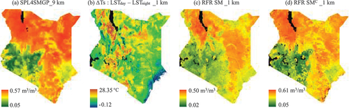
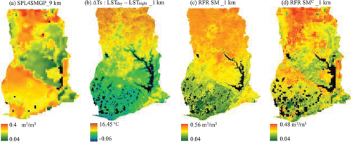
Figure 4. (a) SMAP SM product (SPL4SMGP.007) at 9 km resolution, (b) $\mathrm{\Delta }{\mathrm{T}}_s$ (LST_day-LST_night) calculated using MODIS LST products with 1 km spatial resolution, (c) estimated SM map at 1 km spatial resolution using the proposed RFR method, optical/thermal features, and SM values of SMAP, and (d) 1-km SM^C map after applying the pixel correction equation on the estimated SM for Ghana, Africa.

The outputs of the proposed method for both countries are presented in Figures 3(c) and 4(c). These outputs were calculated using the RFR (which was trained at 9 km spatial resolution) and original RS-related features with the spatial resolution of 1 km in GEE. Based on Figures 3(c) and 4(c), it can be observed that the estimated SM in the two regions of interest exhibits a spatial pattern that lies between the spatial pattern of the SMAP products and other optical/thermal features used to estimate high-resolution SM values in GEE. Overall, the quality and accuracy of the SM estimation process are highly dependent on the availability and quality of the input data, as well as the selection of appropriate land cover types for the estimation process. Given Figures 3(c) and 4(c), the outputs generated from the SM estimation process typically consist of pixels that do not have any estimated values. These pixels are usually limited to those that do not have any data from the optical/thermal and passive microwave observations. Based on the characteristics of passive microwave RS, this limitation of the downscaling method is predominantly related to the lack of data in optical or thermal measurements caused by adverse atmospheric conditions. However, in our study, we utilized the average weekly MODIS data, which contains thermal and vegetation information for most of the pixels. Despite this, there are still some pixels that do not have any estimated SM values. These pixels have been excluded from the estimation process based on the land cover not suited for soil moisture estimation. Additionally, Figures 3(d) and 4(d) show the output of the proposed method after applying correction formula (Eq (3)(3) $\mathit{S}{M}^c\left(\mathrm{i},\mathrm{j}\right)=\mathrm{SM}\left(\mathrm{i},\mathrm{j}\right)+\left[\frac{S{M}_{PMW}^a+\mathit{S}{M}_{PMW}^d}{2}\right]-\frac{1}{N}\sum _{\mathit{i},\mathit{j}}^N\mathrm{SM}\left(\mathrm{i},\mathrm{j}\right)$(3) ) to ensure homogeneity between the results of the RFR and the SMAP product for Kenya and Ghana, respectively.

The proposed method focuses on estimating 1-km SM by considering three crucial factors: 1) main original coarse-scale SM product, which is the 9-km SMAP product, 2) SM-related features with higher spatial resolution, which are derived from MODIS observations, and 3) downscaling method, which is RFR. By leveraging these three factors, the estimation of SM at a resolution of 1 km becomes feasible. It can be said that the observed SM reflects the variations present in all the data used for estimation, including LST, NDVI, LULC, three-band’s reflectance, and the original coarse-scale SM product. However, it is expected that after pixel-mean correction, the spatial pattern and the range of output SM map (Figures 3(d) and 4(d)) are closer to the SMAP product comparing to the initial RFR result (Figures 3(c) and 4(c)). Since SMAP product has been thoroughly examined in a number of research locations (Mohseni et al., 2022), the agreement between the pattern and range of calculated SM and the SMAP observations can be attributable to a major improvement and the success of the downscaling procedure.

However, as can be seen in Figures 3(d) and 4(d), there are two main impacts of this correction visible in the outputs, which may make it less effective compared to the initial RFR retrieved SM. First, as shown in these sub-figures, the SMAP pixel watermark can be observed in the results, which is a fundamental challenge of all SM_PMW downscaling methods. Most of the coarse-scale SMAP pixels can be identified in the results, but this problem does not exist in the estimated SM using the trained RFR. Secondly, there are also more pixels with non-value SM after implementing the correction, due to the non-value pixels in SPL4SMGP.007, as shown by the black areas in Figures 3(d) and 4(d). This issue can pose a challenge in estimating SM values near water bodies, urban areas, and forests, where different landscapes have varying SM values that their spatial and temporal SM information are required for different studies. In conclusion, the correction coefficient can improve the estimated SM values, bringing them closer to the SMAP product. However, the presence of the SM_PMW pixel watermark and the increased number of flags and no data pixels in the results have an inevitable and somewhat destructive effect.

4.2. Statistical evaluation of the proposed method

To statistically evaluate the performance of the proposed method, we compared SM maps generated using the proposed method with in-situ measurements taken over a 1-year period. Figure 5 represents the results of spatial correlation analyses conducted separately for Ghana and Kenya, comparing the outputs of the proposed method with in-situ SM measurements. It should be noted that since SMAP SM values were used to train the RFR, this figure also presents the statistical evaluation of the SM_PMW observation with 9 km resolution. The data used to generate the results in Figure 5 were limited to the weeks and stations where both the RS products/outputs and in-situ measurements were available.

Figure 5. Spatial correlation analyses conducted between the RS-derived SM and in-situ SM measurements, separately for Kenya and Ghana. (a) and (d): SPL4SMGP.007at 9 km spatial resolution, (b) and (e): estimated SM at 1 km before applying pixel-mean correction (Eq (3(3) $\mathit{S}{M}^c\left(\mathrm{i},\mathrm{j}\right)=\mathrm{SM}\left(\mathrm{i},\mathrm{j}\right)+\left[\frac{S{M}_{PMW}^a+\mathit{S}{M}_{PMW}^d}{2}\right]-\frac{1}{N}\sum _{\mathit{i},\mathit{j}}^N\mathrm{SM}\left(\mathrm{i},\mathrm{j}\right)$(3) )), and (c) and (f): SMC at 1 km after applying pixel-mean correction (Eq (3(3) $\mathit{S}{M}^c\left(\mathrm{i},\mathrm{j}\right)=\mathrm{SM}\left(\mathrm{i},\mathrm{j}\right)+\left[\frac{S{M}_{PMW}^a+\mathit{S}{M}_{PMW}^d}{2}\right]-\frac{1}{N}\sum _{\mathit{i},\mathit{j}}^N\mathrm{SM}\left(\mathrm{i},\mathrm{j}\right)$(3) )).

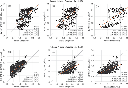
Figure 5 displays the R values, along with the average SM, Bias, RMSD, and ubRMSD measured in m³/m³ units, for each area of interest. In this figure, panels (a) and (d) present the spatial correlation analysis results for the initial SMAP product (SPL4SMGP.007) at a 9 km spatial resolution, which were used for training the RFR in GEE. As can be seen in these sub-figures, the R values between the SMAP products and the measured SM values in Kenya and Ghana are 0.63 and 0.71, respectively, indicating a moderate-to-strong correlation and accuracy for SMAP product. The weekly SMAP observations have an average SM value of 0.32 m³/m³ with a RMSD of 0.089 m³/m³ and ubRMSD of 0.087 m³/m³ in Kenya, while in Ghana, the average SM value is 0.20 m³/m³ with an RMSD of 0.077 m³/m³ and ubRMSD of 0.056 m³/m³.

The results of comparing the RFR outputs with the in-situ measurements at a 1 km spatial resolution are shown in Figures 5(b,e). Based on these figures, the proposed method can estimate weekly SM with correlation coefficient of 0.65 and 0.64 in Kenya and Ghana, respectively. As can be seen, the RMSD values for the proposed method in Kenya and Ghana are 0.082 m³/m³ and 0.095 m³/m³, respectively. Moreover, considering the bias, 0.077 m³/m³ and 0.061 m³/m³ are achieved as ubRMSD for the proposed method in Kenya and Ghana, respectively. The spatial correlation analysis results for the downscaled SM map for Kenya and Ghana after applying the mean-pixel correction are also represented in Figures 5(c,f), respectively. The results indicate that the correlation coefficients do not change in both study areas after applying the correction. Additionally, the RMSD and ubRMSD values of the SM maps after this equation are 0.11 m³/m³ in Kenya and 0.095 m³/m³ and 0.058 m³/m³ in Ghana, respectively.

As discussed in the preceding sections, our downscaling approach utilizes SMAP observations as a reference to train the RFR model at 9 km resolution, enabling the estimation of 1 km SM using GEE. Consequently, the precision of SMAP’s measurements assumes a pivotal role in shaping the accuracy of our method’s outcomes. In Figure 5, we depict the accuracy of 9 km SMAP in both validation sites, highlighting that our method’s capacity to replicate SMAP measurements inherently cannot surpass the precision of the original RS observations. This is due to the absence of in-situ measurements for calibrating input values. Our primary objective centers on augmenting spatial resolution across expansive geographical extents while upholding the accuracy of input data. Hence, the efficacy of the proposed method resides in its capability to extend high-resolution SM estimation to substantial regions, even without in-situ SM data, while preserving the accuracy embedded within the input RS observations. Acknowledging the pursuit of exceptionally high levels of accuracy in SM estimation through RS observation represents a formidable challenge. The nominal accuracy of SMAP’s SM_PMW stands at 0.04 m³/m³ (Entekhabi et al., 2014); however, actual accuracy exhibits variability from 0.04 to 0.13 across diverse global regions (Colliander et al., 2017, 2021; Das et al., 2016; Mohseni et al., 2022). Furthermore, a wealth of research substantiates that various downscaling methods yield Root Mean Square Error (RMSE) values ranging from 0.04 to 0.12 across heterogeneous study areas and temporal frames (Abbaszadeh et al., 2019; Bai et al., 2019; Das et al., 2011; Fang et al., 2022; Hu et al., 2020; Kim et al., 2018; Xu et al., 2022; Zhao et al., 2018). This collective body of work establishes a consistent performance benchmark for downscaling methodologies.

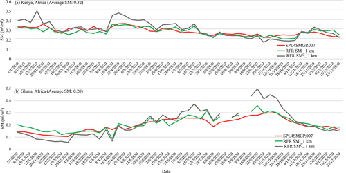
The study examined the temporal patterns of the original SMAP product, as well as the initial output of RFR and the outputs after correction equation (Eq (3)(3) $\mathit{S}{M}^c\left(\mathrm{i},\mathrm{j}\right)=\mathrm{SM}\left(\mathrm{i},\mathrm{j}\right)+\left[\frac{S{M}_{PMW}^a+\mathit{S}{M}_{PMW}^d}{2}\right]-\frac{1}{N}\sum _{\mathit{i},\mathit{j}}^N\mathrm{SM}\left(\mathrm{i},\mathrm{j}\right)$(3) ). The SM trends of these observations were plotted and compared, as shown in Figure 6. Overall, the three maps showed similar trends. For most weeks in Ghana, it was observed that the average SM values of the initial output of RFR were closer to the SMAP data as compared to the outputs after the Eq (3(3) $\mathit{S}{M}^c\left(\mathrm{i},\mathrm{j}\right)=\mathrm{SM}\left(\mathrm{i},\mathrm{j}\right)+\left[\frac{S{M}_{PMW}^a+\mathit{S}{M}_{PMW}^d}{2}\right]-\frac{1}{N}\sum _{\mathit{i},\mathit{j}}^N\mathrm{SM}\left(\mathrm{i},\mathrm{j}\right)$(3) ). Similarly, in Kenya, the initial output of RFR showed closer proximity to the SMAP data than the outputs after Eq (3(3) $\mathit{S}{M}^c\left(\mathrm{i},\mathrm{j}\right)=\mathrm{SM}\left(\mathrm{i},\mathrm{j}\right)+\left[\frac{S{M}_{PMW}^a+\mathit{S}{M}_{PMW}^d}{2}\right]-\frac{1}{N}\sum _{\mathit{i},\mathit{j}}^N\mathrm{SM}\left(\mathrm{i},\mathrm{j}\right)$(3) ), albeit in a lower number of weeks.

Figure 6. Temporal patterns of the original SMAP product with 9 km resolution, the 1 km SM map retrieved from RFR, and the SM map after applying the correction coefficient Eq (3(3) $\mathit{S}{M}^c\left(\mathrm{i},\mathrm{j}\right)=\mathrm{SM}\left(\mathrm{i},\mathrm{j}\right)+\left[\frac{S{M}_{PMW}^a+\mathit{S}{M}_{PMW}^d}{2}\right]-\frac{1}{N}\sum _{\mathit{i},\mathit{j}}^N\mathrm{SM}\left(\mathrm{i},\mathrm{j}\right)$(3) ) for 2020 with in-situ measurements of the Kenya (a) and Ghana (b) validation sites.

The results of our study indicate that the proposed method is highly effective in estimating SM with significantly better spatial resolution compared to the SMAP products with 9 km spatial resolution. Furthermore, the proposed method achieves this improvement almost without sacrificing accuracy. This is a significant development, as it can facilitate the estimation of SM at a continental or global scale, which is typically challenging, time-consuming, and expensive when processing RS data. Despite the promising results of the proposed method, applying the correction equation and using SMAP measurements to correct the estimated values did not lead to any significant improvements in the R, RMSD, and ubRMSD of the estimated SM. These findings indicate that while the correction method may improve the accuracy of the RFR model in some study area and under specific land cover and atmospheric condition, it may not always be necessary or effective in certain regions and time periods.

4.3. The uncertainty of the outputs

In previous studies, the distribution of stations in validation sites has been identified as a crucial factor in validating SM products retrieved from SM_PMW (Beck et al., 2021; Colliander et al., 2017; Mohseni et al., 2022). A similar issue arises when estimating higher spatial resolution SM from these data. In this study, measurements from multiple stations within a coarse scale pixel are averaged and then compared with the coarse-scale values. Similarly, when evaluating SM outputs with higher spatial resolution, the values of each station are compared with the values of pixels on which they are located. In line with this issue, Core Validation Sites (CVSs) have been established to investigate the SMAP and SMOS product performances (Colliander et al., 2017, 2021). However, within Africa, there are no CVSs and the available networks are very sparse, which can introduce limited informative value, particularly when validating the original SM map and the performance of the downscaling procedure.

Different remote sensing satellites are designed with specific spatial and temporal resolutions in accordance with their mission objectives and resource constraints. The MODIS sensor, which we utilized in our study, presents a high temporal resolution of 1 day, enabling daily LST retrievals. Variations in atmospheric conditions may, however, result in observations of LST every 3 days or even longer. Various temporal resolutions as a result of atmospheric conditions can cause uncertainty. Interpolation methods can be employed to estimate LST values on days when direct measurements are unavailable due to atmospheric conditions (Zhao & Duan, 2020; Zhu et al., 2022). However, these interpolation techniques introduce significant uncertainties that can impact the accuracy of downscaling methods. Consequently, this uncertainty could propagate discussions regarding the performance and outcomes of the downscaling method. It should be kept in mind that top layer SM (0–5 cm) values of SPL4SMGP.007 product is used in this study (Chan et al., 2016; Escorihuela et al., 2010; Mohanty et al., 2017). However, the study investigates the results using in-situ SM reference data obtained at 10 cm depth, which may introduce additional uncertainties. At weekly time steps as analyzed in this study, this effect can be regarded as negligible.

5. Conclusion and outlook

This study proposes a workflow using the Google Earth Engine (GEE) to estimate SM at the spatial resolution of 1 km, overcoming the limitation of the tens of kilometers resolution obtained from passive microwave RS observations. The method involves MODIS optical/thermal measurements, SMAP coarse scale SM products, and a Random Forest Regression (RFR) to estimate SM at a higher spatial resolution. The method was applied to the continent of Africa for the year 2020, producing 52 weekly SM maps that were evaluated using in-situ SM measurements from 35 stations across three validation networks. The results indicate that the proposed method can estimate SM at 1 km spatial resolution with acceptable accuracy, with an average correlation coefficient of 0.64 and a ubRMSD of 0.069. The proposed method in GEE can estimate SM at a very good spatial resolution in a nearly expanded area compared to the original SMAP measurement, which had a spatial resolution of 9 km and similar correlation coefficient and RMSD values.

The current study used an averaging method to estimate weekly optical/thermal features, and thereby, weekly SM at a 1 km spatial resolution. However, the temporal heterogeneity of SM especially in croplands is very high, making weekly estimation inadequate for some applications. Therefore, future studies may focus on using interpolation methods to retrieve optical/thermal features at shorter time intervals, such as 2–3 days (the temporal resolution of SMAP) for further implementation in the proposed method to obtain higher temporal resolution SM data for agricultural applications. This can support the improvement of agricultural practices, water resource management, and climate modeling, among other applications.

Disclosure statement

No potential conflict of interest was reported by the author(s).

Data availability statement

All satellite data and products supporting the methodology and findings of this paper (including MODIS and SM Products) have been archived in GEE and are openly available at https://developers.google.com/earth437engine/datasets/catalog/. The field samples of SM over three validation sites, which were used in this study to validate the proposed method, were collected using the ISMN and are available at https://ismn.earth/.

Supplemental data

Supplemental data for this article can be accessed online at https://doi.org/10.1080/20964471.2023.2257905.

Additional information

Funding

The authors were funded by the Deutsche Forschungsgemeinschaft (DFG, German Research Foundation) – SFB 1502/1-2022 – project number: 450058266.

Notes on contributors

Farzane Mohseni

Dr. Ing. Farzane Mohseni is a scientific researcher at the Institute of Geodesy and Geoinformation (Working group Geoinformation) at the University of Bonn since December 2022. Her research interests include soil hydrology, groundwater estimation, water resource management, disaggregation of coarse-scale radiometric soil moisture products, and land cover mapping. She received the B.Sc. degrees in geodesy and geomatics in 2015, the M.Sc. degree in remote sensing in 2017, and a doctoral degree in remote sensing in 2022 from the K. N. Toosi University of Technology, Iran. Prior to assuming her current position, she had been a visiting researcher at the University of Lund, Sweden.

Amirhossein Ahrari

M.Sc. Amirhossein Ahrari holds a position as a PhD researcher in Environmental Engineering, at the University of Oulu, Finland. His primary research focused on hydrological data mining utilizing data from earth observation satellites. With a strong emphasis on enhancing accuracy of hydrological applications, he employs advanced machine learning algorithms to extract valuable insights from satellite data. Prior to his current role, he achieved his Bachelor’s (2015) and Master’s (2018) degrees in Remote Sensing & GIS with specialization in soil and water studies from the University of Tehran, Iran.

Jan-Henrik Haunert

Prof. Dr. Ing. Jan-Henrik Haunert is a full professor of geoinformation at the University of Bonn, Germany. His research is concerned with the development of efficient algorithms for geovisualization and spatial data analytics. In particular, he applies methods from combinatorial optimization and computational geometry to tasks of automated cartography, such as the aggregation and selection of objects in multi-scale digital landscape models. Before he took up his current position, he had acquired a diploma and doctoral degree in geodesy and geoinformatics from the University of Hannover, Germany, had been a postdoctoral researcher at the institute of computer science at the University of Würzburg, Germany, and a professor of geoinformatics at the University of Osnabrück, Germany.

Carsten Montzka

Dr. Carsten Montzka received the Ph.D. degree in geography from the University of Bonn, Germany, in 2007, for the integration of multispectral remote sensing data into nitrogen cycle simulations. In 2004, he joined the Institute of Bio- and Geosciences: Agrosphere (IBG-3) of the Forschungszentrum Jülich, Jülich, Germany. Since 2007, he has been working on passive microwave retrieval for soil moisture and related validation activities. His current work has mainly been focused on the development of multiscale soil moisture data assimilation techniques, airborne active/passive microwave campaigns to support new microwave-based soil moisture missions, and multi-sensor combination on Unmanned Aerial Vehicles (thermal, multispectral, LiDAR). He is alumnus of the Arab-German Young Academy for Sciences and Humanities (AGYA), Berlin, Germany, and is soil moisture focus area co-lead of the Committee on Earth Observation Satellites (CEOS) Land Parameter Validation subgroup.

References

- Abbaszadeh, P., Moradkhani, H., & Zhan, X. (2019). Downscaling SMAP radiometer soil moisture over the CONUS using an ensemble learning method. Water Resources Research, 55(1), 324–344. https://doi.org/10.1029/2018WR023354
- Adab, H., Morbidelli, R., Saltalippi, C., Moradian, M., & Ghalhari, G. A. F. (2020). Machine learning to estimate surface soil moisture from remote sensing data. Water, 12(11), 1–28. https://doi.org/10.3390/w12113223
- Amani, M., Ghorbanian, A., Ahmadi, S. A., Kakooei, M., Moghimi, A., Mirmazloumi, S. M., Moghaddam, S. H. A., Mahdavi, S., Ghahremanloo, M., Parsian, S., Wu, Q., & Brisco, B. (2020). Google Earth Engine cloud computing platform for remote sensing big data applications: A comprehensive review. IEEE Journal of Selected Topics in Applied Earth Observations & Remote Sensing, 13, 5326–5350. https://doi.org/10.1109/JSTARS.2020.3021052
- Anderson, W. B., Zaitchik, B. F., Hain, C. R., Anderson, M. C., Yilmaz, M. T., Mecikalski, J., & Schultz, L. (2012). Towards an integrated soil moisture drought monitor for East Africa. Hydrology and Earth System Sciences, 16(8), 2893–2913. https://doi.org/10.5194/hess-16-2893-2012
- Ardö, J. (2013). A 10-year dataset of basic meteorology and soil properties in central Sudan. Dataset Papers in Geosciences, 2013, 1–6. https://doi.org/10.7167/2013/297973
- Babaeian, E., Sadeghi, M., Jones, S. B., Montzka, C., Vereecken, H., & Tuller, M. (2019). Ground, proximal, and satellite remote sensing of soil moisture. In Reviews of geophysics (Vol. 57, Issue 2, pp. 530–616). Blackwell Publishing Ltd. https://doi.org/10.1029/2018RG000618
- Bai, J., Cui, Q., Zhang, W., & Meng, L. (2019). An approach for downscaling SMAP soil moisture by combining Sentinel-1 SAR and MODIS data. Remote Sensing, 11(23), 2736. https://doi.org/10.3390/rs11232736
- Beck, H. E., Pan, M., Miralles, D. G., Reichle, R. H., Dorigo, W. A., Hahn, S., Sheffield, J., Karthikeyan, L., Balsamo, G., Parinussa, R. M., van Dijk, A. I. J. M., Du, J., Kimball, J. S., Vergopolan, N., & Wood, E. F. (2021). Evaluation of 18 satellite- and model-based soil moisture products using in situ measurements from 826 sensors. Hydrology and Earth System Sciences, 25(1), 17–40. https://doi.org/10.5194/hess-25-17-2021
- Borah, S., Balas, V. E., & Polkowski, Z. (n.d.). Advances in Data Science and Management Lecture Notes on Data Engineering and Communications Technologies 37. http://www.springer.com/series/15362
- Brocca, L., Zhao, W., & Lu, H. (2023). High-resolution observations from space to address new applications in hydrology. The Innovation, 4(3), 100437. https://doi.org/10.1016/j.xinn.2023.100437
- Carlson, T. (2007). An overview of the ‘triangle method’ for estimating surface evapotranspiration and soil moisture from satellite imagery. Sensors, 7(8), 1612–1629. https://doi.org/10.3390/s7081612
- Carlson, T. N., & Petropoulos, G. P. (2019). A new method for estimating of evapotranspiration and surface soil moisture from optical and thermal infrared measurements: The simplified triangle. International Journal of Remote Sensing, 40(20), 7716–7729. https://doi.org/10.1080/01431161.2019.1601288
- Chan, S. K., Bindlish, R., O’Neill, P. E., Njoku, E., Jackson, T., Colliander, A., Chen, F., Burgin, M., Dunbar, S., Piepmeier, J., Yueh, S., Entekhabi, D., Cosh, M. H., Caldwell, T., Walker, J., Wu, X., Berg, A., Rowlandson, T. … Crow, W. T. (2016). Assessment of the SMAP passive soil moisture product. IEEE Transactions on Geoscience and Remote Sensing, 54(8), 4994–5007. https://doi.org/10.1109/TGRS.2016.2561938
- Chen, F., Crow, W. T., Bindlish, R., Colliander, A., Burgin, M. S., Asanuma, J., & Aida, K. (2018). Global-scale evaluation of SMAP, SMOS and ASCAT soil moisture products using triple collocation. Remote Sensing of Environment, 214, 1–13. https://doi.org/10.1016/J.RSE.2018.05.008
- Chul Jung, H., Getirana, A., Arsenault, K. R., Kumar, S., & Maigary, I. (2019). Improving surface soil moisture estimates in West Africa through GRACE data assimilation 2 3. Journal of Hydrology, 575, 192–201. https://doi.org/10.1016/j.jhydrol.2019.05.042
- Colliander, A., Cosh, M. H., Misra, S., Jackson, T. J., Crow, W. T., Chan, S., Bindlish, R., Chae, C., Holifield Collins, C., & Yueh, S. H. (2017). Validation and scaling of soil moisture in a semi-arid environment: SMAP validation experiment 2015 (SMAPVEX15). Remote Sensing of Environment, 196, 101–112. https://doi.org/10.1016/j.rse.2017.04.022
- Colliander, A., Jackson, T. J., Bindlish, R., Chan, S., Das, N., Kim, S. B., Cosh, M. H., Dunbar, R. S., Dang, L., Pashaian, L., Asanuma, J., Aida, K., Berg, A., Rowlandson, T., Bosch, D., Caldwell, T., Caylor, K., Goodrich, D. … Njoku, E. G. (2017). Validation of SMAP surface soil moisture products with core validation sites. Remote Sensing of Environment, 191, 215–231. https://doi.org/10.1016/j.rse.2017.01.021
- Colliander, A., Reichle, R. H., Crow, W. T., Cosh, M. H., Chen, F., Chan, S., Das, N. N., Bindlish, R., Chaubell, J., Kim, S., Liu, Q., O’Neill, P. E., Dunbar, R. S., Dang, L. B., Kimball, J. S., Jackson, T. J., Al-Jassar, H. K., Asanuma, J. … Entekhabi, D. (2021). Validation of soil moisture data products from the NASA SMAP mission. IEEE Journal of Selected Topics in Applied Earth Observations and Remote Sensing, 15, 364–392. https://doi.org/10.1109/JSTARS.2021.3124743
- Das, N. N., Entekhabi, D., Dunbar, R. S., Njoku, E. G., & Yueh, S. H. (2016). Uncertainty estimates in the SMAP combined active-passive downscaled brightness temperature. IEEE Transactions on Geoscience and Remote Sensing, 54(2), 640–650. https://doi.org/10.1109/TGRS.2015.2450694
- Das, N. N., Entekhabi, D., & Njoku, E. G. (2011). An algorithm for merging SMAP radiometer and radar data for high-resolution soil-moisture retrieval. IEEE Transactions on Geoscience and Remote Sensing, 49(5), 1504–1512. https://doi.org/10.1109/TGRS.2010.2089526
- de Jeu, R. A. M., Holmes, T. R. H., Parinussa, R. M., & Owe, M. (2014). A spatially coherent global soil moisture product with improved temporal resolution. Journal of Hydrology, 516, 284–296. https://doi.org/10.1016/j.jhydrol.2014.02.015
- Djamai, N., Magagi, R., Goïta, K., Merlin, O., Kerr, Y., & Roy, A. (2016). A combination of DISPATCH downscaling algorithm with CLASS land surface scheme for soil moisture estimation at fine scale during cloudy days. Remote Sensing of Environment, 184, 1–14. https://doi.org/10.1016/j.rse.2016.06.010
- Dorigo, W., Himmelbauer, I., Aberer, D., Schremmer, L., Petrakovic, I., Zappa, L., Preimesberger, W., Xaver, A., Annor, F., Ardö, J., Baldocchi, D., Bitelli, M., Blöschl, G., Bogena, H., Brocca, L., Calvet, J. C., Camarero, J. J., Capello, G., Choi, M., Sabia, R. (2021). The international soil moisture network: Serving earth system science for over a decade. Hydrology and Earth System Sciences, 25(11), 5749–5804. https://doi.org/10.5194/hess-25-5749-2021
- Entekhabi, D., Yueh, S., O’Neill, P. E., Kellogg, K. H., Allen, A., Bindlish, R., & West, R. (2014). SMAP handbook–soil moisture active passive: Mapping soil moisture and freeze/thaw from space. Jet Propulsion Laboratory, California Institute of Technology. https://smap.jpl.nasa.gov/
- Escorihuela, M. J., Chanzy, A., Wigneron, J. P., & Kerr, Y. H. (2010). Effective soil moisture sampling depth of L-band radiometry: A case study. Remote Sensing of Environment, 114(5), 995–1001. https://doi.org/10.1016/j.rse.2009.12.011
- Fang, B., Lakshmi, V., Bindlish, R., & Jackson, T. J. (2018). Downscaling of SMAP soil moisture using land surface temperature and vegetation data. Vadose Zone Journal, 17(1), 1–15. https://doi.org/10.2136/vzj2017.11.0198
- Fang, B., Lakshmi, V., Bindlish, R., Jackson, T. J., Cosh, M., & Basara, J. (2013). Passive microwave soil moisture downscaling using vegetation Index and skin surface temperature. Vadose Zone Journal, 12(3), vzj2013.05.0089. https://doi.org/10.2136/vzj2013.05.0089er
- Fang, B., Lakshmi, V., Cosh, M., Liu, P., Bindlish, R., & Jackson, T. J. (2022). A global 1‐km downscaled SMAP soil moisture product based on thermal inertia theory. Vadose Zone Journal, 21(2), e20182. https://doi.org/10.1002/vzj2.20182
- Fontanet, M., Fernàndez-Garcia, D., & Ferrer, F. (2018). The value of satellite remote sensing soil moisture data and the DISPATCH algorithm in irrigation fields. Hydrology and Earth System Sciences, 22(11), 5889–5900. https://doi.org/10.5194/hess-22-5889-2018
- Gevaert, A. I., Parinussa, R. M., Renzullo, L. J., van Dijk, A. I. J. M., & de Jeu, R. A. M. (2016). Spatio-temporal evaluation of resolution enhancement for passive microwave soil moisture and vegetation optical depth. International Journal of Applied Earth Observation and Geoinformation, 45, 235–244. https://doi.org/10.1016/j.jag.2015.08.006
- Ghafari, E., Walker, J. P., Das, N. N., Davary, K., Faridhosseini, A., Wu, X., & Zhu, L. (2020). On the impact of C-band in place of L-band radar for SMAP downscaling. Remote Sensing of Environment, 251, 112111. https://doi.org/10.1016/J.RSE.2020.112111
- Ghorbanian, A., Kakooei, M., Amani, M., Mahdavi, S., Mohammadzadeh, A., & Hasanlou, M. (2020). Improved land cover map of Iran using sentinel imagery within Google Earth Engine and a novel automatic workflow for land cover classification using migrated training samples. Isprs Journal of Photogrammetry & Remote Sensing, 167, 276–288. https://doi.org/10.1016/J.ISPRSJPRS.2020.07.013
- Gruber, A., De Lannoy, G., Albergel, C., Al-Yaari, A., Brocca, L., Calvet, J. C., Colliander, A., Cosh, M., Crow, W., Dorigo, W., Draper, C., Hirschi, M., Kerr, Y., Konings, A., Lahoz, W., McColl, K., Montzka, C., Muñoz-Sabater, J., Wigneron, J. P. (2020). Validation practices for satellite soil moisture retrievals: What are (the) errors? Remote Sensing of Environment, 244, 111806. https://doi.org/10.1016/j.rse.2020.111806
- Han, Y., Wang, Y., & Zhao, Y. (2010). Estimating soil moisture conditions of the greater changbai mountains by land surface temperature and NDVI. IEEE Transactions on Geoscience and Remote Sensing, 48(6), 2509–2515. https://doi.org/10.1109/TGRS.2010.2040830
- Hu, F., Wei, Z., Zhang, W., Dorjee, D., & Meng, L. (2020). A spatial downscaling method for SMAP soil moisture through visible and shortwave-infrared remote sensing data. Journal of Hydrology, 590, 125360. https://doi.org/10.1016/j.jhydrol.2020.125360
- Jagdhuber, T., Baur, M., Akbar, R., Das, N. N., Link, M., He, L., & Entekhabi, D. (2019). Estimation of active-passive microwave covariation using SMAP and Sentinel-1 data. Remote Sensing of Environment, 225, 458–468. https://doi.org/10.1016/J.RSE.2019.03.021
- Jung, C., Lee, Y., Cho, Y., & Kim, S. (2017). A study of spatial soil moisture estimation using a multiple linear regression model and MODIS land surface temperature data corrected by conditional merging. Remote Sensing, 9(8), 870. https://doi.org/10.3390/rs9080870
- Khazaei, M., Hamzeh, S., Samani, N. N., Muhuri, A., Goïta, K., & Weng, Q. (2023). A web-based system for satellite-based high-resolution global soil moisture maps. Computers and Geosciences, 170, 170. https://doi.org/10.1016/j.cageo.2022.105250
- Khellouk, R., Barakat, A., Boudhar, A., Hadria, R., Lionboui, H., el Jazouli, A., Rais, J., el Baghdadi, M., & Benabdelouahab, T. (2020). Spatiotemporal monitoring of surface soil moisture using optical remote sensing data: A case study in a semi-arid area. Journal of Spatial Science, 65(3), 481–499. https://doi.org/10.1080/14498596.2018.1499559
- Kim, G., & Barros, A. P. (2002). Downscaling of remotely sensed soil moisture with a modified fractal interpolation method using contraction mapping and ancillary data. Remote Sensing of Environment, 83(3), 400–413. https://doi.org/10.1016/S0034-4257(02)00044-5
- Kim, H., Parinussa, R., Konings, A. G., Wagner, W., Cosh, M. H., Lakshmi, V., Zohaib, M., & Choi, M. (2018). Global-scale assessment and combination of SMAP with ASCAT (active) and AMSR2 (passive) soil moisture products. Remote Sensing of Environment, 204, 260–275. https://doi.org/10.1016/j.rse.2017.10.026
- Lievens, H., Tomer, S. K., Al Bitar, A., De Lannoy, G. J. M., Drusch, M., Dumedah, G., Franssen, H.-J. H., Kerr, Y. H., Martens, B., Pan, M., Roundy, J. K., Vereecken, H., Walker, J. P., Wood, E. F., Verhoest, N. E. C., & Pauwels, V. R. N. (2015). SMOS soil moisture assimilation for improved hydrologic simulation in the Murray Darling Basin, Australia. Remote Sensing of Environment, 168, 146–162. https://doi.org/10.1016/j.rse.2015.06.025
- Malbéteau, Y., Merlin, O., Molero, B., Rüdiger, C., & Bacon, S. (2016). DisPATCh as a tool to evaluate coarse-scale remotely sensed soil moisture using localized in situ measurements: Application to SMOS and AMSR-E data in Southeastern Australia. International Journal of Applied Earth Observation and Geoinformation, 45, 221–234. https://doi.org/10.1016/j.jag.2015.10.002
- Ma, H., Zeng, J., Chen, N., Zhang, X., Cosh, M. H., & Wang, W. (2019). Satellite surface soil moisture from SMAP, SMOS, AMSR2 and ESA CCI: A comprehensive assessment using global ground-based observations. Remote Sensing of Environment, 231, 111215. https://doi.org/10.1016/J.RSE.2019.111215
- McNally, A., Shukla, S., Arsenault, K. R., Wang, S., Peters-Lidard, C. D., & Verdin, J. P. (2016). Evaluating ESA CCI soil moisture in East Africa. International Journal of Applied Earth Observation and Geoinformation, 48, 96–109. https://doi.org/10.1016/j.jag.2016.01.001
- Mecklenburg, S., Drusch, M., Kerr, Y. H., Font, J., Martin-Neira, M., Delwart, S., Buenadicha, G., Reul, N., Daganzo-Eusebio, E., Oliva, R., & Crapolicchio, R. (2012). ESA’s soil moisture and ocean salinity mission: Mission performance and operations. IEEE Transactions on Geoscience and Remote Sensing, 50(5), 1354–1366. https://doi.org/10.1109/TGRS.2012.2187666
- Merlin, O., Al Bitar, A., Walker, J. P., & Kerr, Y. (2010). An improved algorithm for disaggregating microwave-derived soil moisture based on red, near-infrared and thermal-infrared data. Remote Sensing of Environment, 114(10), 2305–2316. https://doi.org/10.1016/j.rse.2010.05.007
- Merlin, O., Chehbouni, A. G., Kerr, Y. H., Njoku, E. G., & Entekhabi, D. (2005). A combined modeling and multispectral/multiresolution remote sensing approach for disaggregation of surface soil moisture: Application to SMOS configuration. IEEE Transactions on Geoscience and Remote Sensing, 43(9), 2036–2050. https://doi.org/10.1109/TGRS.2005.853192
- Merlin, O., Walker, J. P., Chehbouni, A., & Kerr, Y. (2008). Towards deterministic downscaling of SMOS soil moisture using MODIS derived soil evaporative efficiency. Remote Sensing of Environment, 112(10), 3935–3946. https://doi.org/10.1016/j.rse.2008.06.012
- Mirmazloumi, S. M., Kakooei, M., Mohseni, F., Ghorbanian, A., Amani, M., Crosetto, M., & Monserrat, O. (2022). ELULC‐10, a 10 m European land use and land cover map using Sentinel and Landsat data in Google Earth Engine. Remote Sensing, 14(13). https://doi.org/10.3390/rs14133041
- Mirmazloumi, S. M., Sahebi, M. R., & Amani, M. (2021). New empirical backscattering models for estimating bare soil surface parameters. International Journal of Remote Sensing, 42(5), 1928–1947. https://doi.org/10.1080/01431161.2020.1847353
- Mohanty, B. P., Cosh, M. H., Lakshmi, V., & Montzka, C. (2017). Soil moisture remote sensing: State-of-the-science. Vadose Zone Journal, 16(1), 1–9. https://doi.org/10.2136/vzj2016.10.0105
- Mohseni, F., Kiani Sadr, M., Eslamian, S., Areffian, A., & Khoshfetrat, A. (2021). Spatial and temporal monitoring of drought conditions using the satellite rainfall estimates and remote sensing optical and thermal measurements. Advances in Space Research, 67(12), 3942–3959. https://doi.org/10.1016/J.ASR.2021.02.017
- Mohseni, F., Mirmazloumi, S. M., Mokhtarzade, M., Jamali, S., & Homayouni, S. (2022). Global evaluation of SMAP/Sentinel-1 soil moisture products. Remote Sensing, 14(18), 4624. https://doi.org/10.3390/rs14184624
- Mohseni, F., & Mokhtarzade, M. (2020). A new soil moisture index driven from an adapted long-term temperature-vegetation scatter plot using MODIS data. Journal of Hydrology, 581, 124420. https://doi.org/10.1016/j.jhydrol.2019.124420
- Mohseni, F., & Mokhtarzade, M. (2021). The synergistic use of microwave coarse-scale measurements and two adopted high-resolution indices driven from long-term T-V scatter plot for fine-scale soil moisture estimation. GIScience and Remote Sensing, 58(3), 455–482. https://doi.org/10.1080/15481603.2021.1906056
- Montzka, C., Cosh, M., Nickeson, J., Camacho, F., Bayat, B., Al Bitar, A., Berg, A., Bindlish, R., Bogena, H. R., & Bolten, J. D. (2021). Soil Moisture Product Validation Good Practices Protocol, Committee on Earth Observation Satellites Working Group on Calibration and Validation Land Product Validation Subgroup, Version 1.0. https://ntrs.nasa.gov.
- Montzka, C., Jagdhuber, T., Horn, R., Bogena, H. R., Hajnsek, I., Reigber, A., & Vereecken, H. (2016). Investigation of SMAP fusion algorithms with airborne active and passive L-band microwave remote sensing. IEEE Transactions on Geoscience and Remote Sensing, 54(7), 3878–3889. https://doi.org/10.1109/TGRS.2016.2529659
- Montzka, C., Rötzer, K., Bogena, H. R., Sanchez, N., & Vereecken, H. (2018). A new soil moisture downscaling approach for SMAP, SMOS, and ASCAT by predicting sub-grid variability. Remote Sensing, 10(3), 427. https://doi.org/10.3390/rs10030427
- Montzka, C., Rötzer, K., Bogena, H. R., Sanchez, N., & Vereecken, H. (2021). A New soil moisture downscaling approach for SMAP, SMOS, and ASCAT by predicting sub-grid variability. https://doi.org/10.1594/PANGAEA.878889
- Mutanga, O., & Kumar, L. (2019). Google Earth Engine applications. Remote Sensing, 11(5), 591. https://doi.org/10.3390/rs11050591
- Myeni, L., Moeletsi, M. E., & Clulow, A. D. (2019). Present status of soil moisture estimation over the African continent. Journal of Hydrology: Regional Studies, 21, 14–24. https://doi.org/10.1016/J.EJRH.2018.11.004
- Narayan, U., & Lakshmi, V. (2008). Characterizing subpixel variability of low resolution radiometer derived soil moisture using high resolution radar data. Water Resources Research, 44(6). https://doi.org/10.1029/2006WR005817
- Naz, B. S., Kollet, S., Franssen, H. J. H., Montzka, C., & Kurtz, W. (2020). A 3 km spatially and temporally consistent European daily soil moisture reanalysis from 2000 to 2015. Scientific Data, 7(1). https://doi.org/10.1038/s41597-020-0450-6
- Neuhauser, M., Verrier, S., Merlin, O., Molero, B., Suere, C., & Mangiarotti, S. (2019). Multi-scale statistical properties of disaggregated SMOS soil moisture products in Australia. Advances in Water Resources, 134, 134. https://doi.org/10.1016/j.advwatres.2019.103426
- Nichols, S. (2011). Review and evaluation of remote sensing methods for soil-moisture estimation. Journal of Photonics for Energy, 028001. https://doi.org/10.1117/1.3534910
- Pellenq, J., Kalma, J., Boulet, G., Saulnier, G. M., Wooldridge, S., Kerr, Y., & Chehbouni, A. (2003). A disaggregation scheme for soil moisture based on topography and soil depth. Journal of Hydrology, 276(1–4), 112–127. https://doi.org/10.1016/S0022-1694(03)00066-0
- Peng, J., Albergel, C., Balenzano, A., Brocca, L., Cartus, O., Cosh, M. H., Crow, W. T., Dabrowska-Zielinska, K., Dadson, S., Davidson, M. W. J., de Rosnay, P., Dorigo, W., Gruber, A., Hagemann, S., Hirschi, M., Kerr, Y. H., Lovergine, F., Mahecha, M. D., Marzahn, P., Loew, A. (2021). A roadmap for high-resolution satellite soil moisture applications – confronting product characteristics with user requirements. Remote Sensing of Environment, 252, 112162. https://doi.org/10.1016/j.rse.2020.112162
- Peng, J., Loew, A., Merlin, O., & Verhoest, N. E. C. (2017). A review of spatial downscaling of satellite remotely sensed soil moisture. Reviews of Geophysics, 55(2), 341–366. https://doi.org/10.1002/2016RG000543
- Petropoulos, G. P., Ireland, G., & Barrett, B. (2015). Surface soil moisture retrievals from remote sensing: Current status, products & future trends. Physics and Chemistry of the Earth, Parts A/B/C, 83, 36–56. https://doi.org/10.1016/j.pce.2015.02.009
- Piles, M., Camps, A., Vall-Llossera, M., Corbella, I., Panciera, R., Rudiger, C., Kerr, Y. H., & Walker, J. (2011). Downscaling SMOS-derived soil moisture using MODIS visible/infrared data. IEEE Transactions on Geoscience and Remote Sensing, 49(9), 3156–3166. https://doi.org/10.1109/TGRS.2011.2120615
- Piles, M., Camps, A., Vall-Llossera, M., Sánchez, N., Martínez-Fernández, J., Monerris, A., Baroncini-Turricchia, G., Pérez-Gutiérrez, C., Aguasca, A., Acevo, R., & Bosch-Lluís, X. (2010). Soil moisture downscaling activities at the REMEDHUS Cal/Val site and its application to SMOS. 2010 11th Specialist Meeting on Microwave Radiometry and Remote Sensing of the Environment, 17–21. https://doi.org/10.1109/MICRORAD.2010.5559599
- Piles, M., Petropoulos, G. P., Sánchez, N., González-Zamora, Á., & Ireland, G. (2016). Towards improved spatio-temporal resolution soil moisture retrievals from the synergy of SMOS and MSG SEVIRI spaceborne observations. Remote Sensing of Environment, 180, 403–417. https://doi.org/10.1016/j.rse.2016.02.048
- Piou, C., Gay, P. E., Benahi, A. S., Babah Ebbe, M. A. O., Chihrane, J., Ghaout, S., Cisse, S., Diakite, F., Lazar, M., Cressman, K., Merlin, O., Escorihuela, M. J., & Mcinnis‐Ng, C. (2019). Soil moisture from remote sensing to forecast desert locust presence. Journal of Applied Ecology, 56(4), 966–975. https://doi.org/10.1111/1365-2664.13323
- Pradhan, S. N., Anjum, M., & Jena, P. (2018). Estimation of soil moisture content by remote sensing methods: A review. Journal of Pharmacognosy & Phytochemistry, 7(1S), 1786–1792.
- Qu, Y., Zhu, Z., Montzka, C., Chai, L., Liu, S., Ge, Y., Liu, J., Lu, Z., He, X., Zheng, J., & Han, T. (2021). Inter-comparison of several soil moisture downscaling methods over the Qinghai-Tibet Plateau, China. Journal of Hydrology, 592, 125616. https://doi.org/10.1016/j.jhydrol.2020.125616
- Reichle, R. H., Liu, Q., Koster, R. D., Ardizzone, J. V., Colliander, A., Crow, W. T., De Lannoy, G. J. M., & Kimball, J. S. (2022). Soil moisture active passive (SMAP) project assessment report for version 6 of the L4_SM data product. Technical Report Series on Global Modeling and Data Assimilation, 60.
- Sabaghy, S., Walker, J. P., Renzullo, L. J., & Jackson, T. J. (2018). Spatially enhanced passive microwave derived soil moisture: Capabilities and opportunities. Remote Sensing of Environment, 209, 551–580. https://doi.org/10.1016/j.rse.2018.02.065
- Sahaar, S. A., Niemann, J. D., & Elhaddad, A. (2022). Using regional characteristics to improve uncalibrated estimation of rootzone soil moisture from optical/thermal remote-sensing. Remote Sensing of Environment, 273, 112982. https://doi.org/10.1016/j.rse.2022.112982
- Sánchez-Ruiz, S., Piles, M., Sánchez, N., Martínez-Fernández, J., Vall-Llossera, M., & Camps, A. (2014). Combining SMOS with visible and near/shortwave/thermal infrared satellite data for high resolution soil moisture estimates. Journal of Hydrology, 516, 273–283. https://doi.org/10.1016/j.jhydrol.2013.12.047
- Seneviratne, S. I., Lüthi, D., Litschi, M., & Schär, C. (2006). Land-atmosphere coupling and climate change in Europe. Nature, 443(7108), 205–209. https://doi.org/10.1038/nature05095
- Shin, Y., & Mohanty, B. P. (2013). Development of a deterministic downscaling algorithm for remote sensing soil moisture footprint using soil and vegetation classifications. Water Resources Research, 49(10), 6208–6228. https://doi.org/10.1002/wrcr.20495
- Song, C., Jia, L., & Menenti, M. (2013). Retrieving high-resolution surface soil moisture by downscaling AMSR-E brightness temperature using MODIS LST and NDVI data. IEEE Journal of Selected Topics in Applied Earth Observations and Remote Sensing, 7(3), 935–942. https://doi.org/10.1109/JSTARS.2013.2272053
- Srivastava, P. K., Han, D., Ramirez, M. R., & Islam, T. (2013). Machine learning techniques for downscaling SMOS satellite soil moisture using MODIS land surface temperature for hydrological application. Water Resources Management, 27(8), 3127–3144. https://doi.org/10.1007/s11269-013-0337-9
- Tamiminia, H., Salehi, B., Mahdianpari, M., Quackenbush, L., Adeli, S., & Brisco, B. (2020). Google Earth Engine for geo-big data applications: A meta-analysis and systematic review. ISPRS Journal of Photogrammetry & Remote Sensing, 164, 152–170. https://doi.org/10.1016/J.ISPRSJPRS.2020.04.001
- van de Giesen, N., Hut, R., & Selker, J. (2014). The Trans‐African hydro‐meteorological observatory (TAHMO). WIREs Water, 1(4), 341–348. https://doi.org/10.1002/wat2.1034
- Vereecken, H., Huisman, J. A., Pachepsky, Y., Montzka, C., van der Kruk, J., Bogena, H., Weihermüller, L., Herbst, M., Martinez, G., & Vanderborght, J. (2014). On the spatio-temporal dynamics of soil moisture at the field scale. Journal of Hydrology, 516, 76–96. https://doi.org/10.1016/J.JHYDROL.2013.11.061
- Wang, W., Huang, D., Wang, X. G., Liu, Y. R., & Zhou, F. (2011). Estimation of soil moisture using trapezoidal relationship between remotely sensed land surface temperature and vegetation index. Hydrology and Earth System Sciences, 15(5), 1699–1712. https://doi.org/10.5194/hess-15-1699-2011
- Xu, C., Qu, J. J., Hao, X., Cosh, M. H., Prueger, J. H., Zhu, Z., & Gutenberg, L. (2018). Downscaling of surface soil moisture retrieval by combining MODIS/Landsat and in situ measurements. Remote Sensing, 10(2), 210. https://doi.org/10.3390/rs10020210
- Xu, Y., Wang, L., Ma, Z., Li, B., Bartels, R., Liu, C., Zhang, X., & Dong, J. (2020). Spatially explicit model for statistical downscaling of satellite passive microwave soil moisture. IEEE Transactions on Geoscience and Remote Sensing, 58(2), 1182–1191. https://doi.org/10.1109/TGRS.2019.2944421
- Xu, M., Yao, N., Yang, H., Xu, J., Hu, A., de Goncalves, L. G. G., & Liu, G. (2022). Downscaling SMAP soil moisture using a wide & deep learning method over the continental United States. Journal of Hydrology, 609, 127784. https://doi.org/10.1016/j.jhydrol.2022.127784
- Xu, W., Zhang, Z., Long, Z., & Qin, Q. (2021). Downscaling SMAP soil moisture products with convolutional neural network. IEEE Journal of Selected Topics in Applied Earth Observations and Remote Sensing, 14, 4051–4062. https://doi.org/10.1109/JSTARS.2021.3069774
- Zhao, W., & Duan, S. B. (2020). Reconstruction of daytime land surface temperatures under cloud-covered conditions using integrated MODIS/Terra land products and MSG geostationary satellite data. Remote Sensing of Environment, 247, 111931. https://doi.org/10.1016/j.rse.2020.111931
- Zhao, W., Sánchez, N., Lu, H., & Li, A. (2018). A spatial downscaling approach for the SMAP passive surface soil moisture product using random forest regression. Journal of Hydrology, 563, 1009–1024. https://doi.org/10.1016/j.jhydrol.2018.06.081
- Zhao, W., Wen, F., Wang, Q., Sanchez, N., & Piles, M. (2021). Seamless downscaling of the ESA CCI soil moisture data at the daily scale with MODIS land products. Journal of Hydrology, 603, 126930. https://doi.org/10.1016/J.JHYDROL.2021.126930
- Zheng, J., Lü, H., Crow, W. T., Zhao, T., Merlin, O., Rodriguez-Fernandez, N., Shi, J., Zhu, Y., Su, J., Kang, C. S., Wang, X., & Gou, Q. (2021a). Soil moisture downscaling using multiple modes of the DISPATCH algorithm in a semi-humid/humid region. International Journal of Applied Earth Observation and Geoinformation, 104, 102530. https://doi.org/10.1016/j.jag.2021.102530
- Zheng, J., Lü, H., Crow, W. T., Zhao, T., Merlin, O., Rodriguez-Fernandez, N., Shi, J., Zhu, Y., Su, J., Kang, C. S., Wang, X., & Gou, Q. (2021b). Soil moisture downscaling using multiple modes of the DISPATCH algorithm in a semi-humid/humid region. International Journal of Applied Earth Observation and Geoinformation, 104, 102530. https://doi.org/10.1016/j.jag.2021.102530
- Zhu, X., Duan, S. B., Li, Z. L., Wu, P., Wu, H., Zhao, W., & Qian, Y. (2022). Reconstruction of land surface temperature under cloudy conditions from Landsat 8 data using annual temperature cycle model. Remote Sensing of Environment, 281, 113261. https://doi.org/10.1016/j.rse.2022.113261
- Zreda, M., Shuttleworth, W. J., Zeng, X., Zweck, C., Desilets, D., Franz, T., & Rosolem, R. (2012). COSMOS: The cosmic-ray soil moisture observing system. Hydrology and Earth System Sciences, 16(11), 4079–4099. https://doi.org/10.5194/hess-16-4079-2012
- Zribi, M., Andre, C., & Decharme, B. (2008). A method for soil moisture estimation in Western Africa based on the ERS scatterometer. IEEE Transactions on Geoscience and Remote Sensing, 46(2), 438–448. https://doi.org/10.1109/TGRS.2007.904582
- Zribi, M., Foucras, M., Baghdadi, N., Demarty, J., & Muddu, S. (2020). A new reflectivity index for the retrieval of surface soil moisture from radar data. IEEE Journal of Selected Topics in Applied Earth Observations and Remote Sensing, 14, 818–826. https://doi.org/10.1109/JSTARS.2020.3033132