Predicting Larch Casebearer damage with confidence using Yolo network models and conformal prediction

ABSTRACT

This investigation shows that successful forecasting models for monitoring forest health status with respect to Larch Casebearer damages can be derived using a combination of a confidence predictor framework (Conformal Prediction) in combination with a deep learning architecture (Yolo v5). A confidence predictor framework can predict the current types of diseases used to develop the model and also provide indication of new, unseen, types or degrees of disease. The user of the models is also, at the same time, provided with reliable predictions and a well-established applicability domain for the model where such reliable predictions can and cannot be expected. Furthermore, the framework gracefully handles class imbalances without explicit over- or under-sampling or category weighting which may be of crucial importance in cases of highly imbalanced datasets. The present approach also provides indication of when insufficient information has been provided as input to the model at the level of accuracy (reliability) need by the user to make subsequent decisions based on the model predictions.

KEYWORDS:

• Yolo network
• Larch Casebearer moth
• conformal prediction
• forest health
• tree damage

1. Introduction

The acquisition and analysis of visual imagery using remote-sensing data from satellites, aircraft, and Unmanned Aerial Vehicles (UAVs) is common for many applications in forestry (Diez et al. 2021; Hoeser and Kuenzer 2020; Hoeser, Bachofer, and Kuenzer 2020). It can be used to classify forest species (Zhang et al. 2020), for change detection (Shi et al. 2020), forest fire detection (Hossain, Zhang, and Akter Tonima 2020; Zhao et al. 2018) and tree health classification due to insect infestations (Barmpoutis, Kamperidou, and Stathaki 2020; Deng et al. 2020; Minařík, Langhammer, and Lendzioch 2021; Nguyen et al. 2021).

Current state-of-the-art image classification and detection techniques use machine learning to build models that relate the incoming image data to the set of class labels (Szeliski 2011). Due to the typical complexity of image data – images may have many millions of pixels – the most successful image classification and detection systems are based on upon Deep Learning (DL) systems that use neural network architectures with many layers (Russakovsky et al. 2015) Deep learning networks contain millions of parameters that are tuned via a training phase and learn very complex representations of visual images (LeCun, Bengio, and Hinton 2015; Schmidhuber 2015).

Deep learning is frequently used for automated classification and detection tasks in remote sensing (Diez et al. 2021; Hamedianfar et al. 2022; Reichstein et al. 2019; Zhu et al. 2017).

However, there are issues with using automated classification and detection systems. Much of the available research only presents results on small test sets, which means that it is not clear how well the prediction models can generalize to previously unseen data; that is, data outside the training set (Diez et al. 2021; Hamedianfar et al. 2022). In other words, the model may be overfitted to the training set (Hamedianfar et al. 2022). Furthermore, the test sets need to be completely isolated from the training sets and this is not always the case (Diez et al. 2021) Another issue with using deep learning models for remote sensing is that these models are sensitive to class imbalance (Kattenborn et al. 2021). Class imbalance occurs when different classes do not have the same size (Johnson and Khoshgoftaar 2019). If standard measures of overall accuracy are used in an imbalanced dataset, then the results can be biased (Kattenborn et al. 2021).

This article demonstrates how the problems of generalization and class imbalance can be addressed using a classification framework known as Conformal Prediction. Conformal prediction provides a statistically guaranteed measure of confidence for each prediction from a classification system (Vovk, Gammerman, and Shafer 2005). As a result, it can provide unbiased predictions for imbalanced datasets, even if the imbalance is as severe as 1:1000 (Norinder and Boyer 2017) and will automatically identify if the prediction system cannot successfully generalize to the examples, e.g., images, it needs to classify (Fisch et al. 2022)

Conformal prediction makes no assumptions about the underlying model it is evaluating, and thus can be used with virtually any machine learning or deep learning classification or detection algorithm. In this article, it is integrated with the Yolo v5 detection network (Jocher et al. 2022), but it has also been demonstrated with a wide range of other image classification systems (Angelopoulos et al. 2021).

Conformal prediction has been used in a wide range of applications such as cancer diagnosis (Olsson et al. 2022), drug design (Norinder et al. 2014), anomaly detection in ship traffic (Laxhammar and Falkman 2010), clinical medicine (Vazquez and Facelli 2022), and to predict drug resistance (Hernández-Hernández, Vishwakarma, and Ballester 2022). However, conformal prediction is rarely used in remote sensing applications.

This article presents a method of predicting damages caused by the Larch Casebearer moth using a deep learning model within a conformal prediction framework, from colour images collected using an Unmanned Aerial Vehicle (UAV). It demonstrates that using a conformal prediction framework allows reliable predictions of Larch Casebearer damages and predict the appearance of new and previously unseen degrees of disease. The framework gracefully handles a dataset that contains considerable class imbalance (in this dataset, more than 70% of the training data comes from just one of the three classification classes). Furthermore, the conformal prediction framework provides an indication of when insufficient information has been provided to the model to reliably base decisions on the model predictions.

2. Materials and methods

2.1. Dataset

The dataset was obtained from the Swedish Forest Agency (https://skogsdatalabbet.se/delning_av_ai_larksackmal/, accessed 25 November 2022) and LILA BC (https://lila.science/datasets/forest-damages-larch-casebearer/, accessed 25 November 2022). The dataset contains 1543 images obtained from drones flying over five affected areas in Västergötland, Sweden, by the larch casebearer, a moth that damages larch trees, and consists of 10 batches. The bounding box annotations around trees in the batches are categorized as Larch and Other. Only batches 1–5, containing bounding box annotations categorized as Larch, were used for this investigation. These batches contain three categories of tree annotations: Healthy (H), Light Damage (LD) and High Damage (HD). The bounding boxes identified by the Swedish Forest Agency project (Radogoshi 2021) were used in this analysis. Some very small bounding boxes, also identified by the project, were removed. In this study, boxes with <10 pixels in either dimension were removed.

The final dataset used for analysis contained 44,980 bounding boxes (HD: 9066, LD: 33276, H: 2638). The dataset was first randomly split into training and test set (70/30) for each category and each training set was subsequently randomly split into a final training and validation set (90/10) for each category (see Table 1).

Table 1. Number of bounding boxes used in the original three category datasets. The dataset is heavily imbalanced towards the Light Damage (LD) class.

	Class
Set	H	LD	HD	Total
Training	1661	20956	5704	28321
Validation	185	2331	636	3152
Test	792	9989	2726	13507

The original three category dataset was also divided into several binary classification datasets (see Table 2). It can be useful to simplify multi-class models into binary class models as the latter can be more predictive than the former. The selection of how to divide the classes into a binary setting depends on which class decision is more relevant or significant, and how much error can be tolerated. This is illustrated in Table 2 where for the ‘H_vs_LHD’ model it is more important to identify the ‘H’ class while for the ‘HLD_vs_HD’ model the ‘HD’ category is the class of importance.

Table 2. Binary data sets from the original three category dataset.

Model	Category 1	Category 2	Comments
H_vs_LHD	H	LD+HD
HLD_vs_HD	H+LD	HD
H_vs_HD	H	HD	No LD bounding boxes^a

^aThe test set with LD bounding boxes was used as additional external test sets of the model.

2.2. Deep learning method

The classification models were developed using the Yolo v5 network model and code obtained from Ultralytics GitHub repository yolov5 (https://github.com/ultralytics/yolov5, accessed 27 October 2022). YOLO v5 architecture consists of four parts: input, backbone, neck, and output. The input part performs preprocessing of the images as well as image augmentation. The backbone is a cross-stage partial network (CSP) architecture for extracting image features. The neck uses a feature pyramid network (FPN) and a path aggregation network (PAN) for improving the extracted features while the output part is a convolution layer for presenting output results, e.g., classes or scores. The pretrained Yolo yolov5s-cls network and default settings were used for the fine tuning (training) of the models in this study.

2.3. Conformal prediction

Image classification produces a classifier that, for an image , output scores for a set of possible classes . Such classifiers do not provide a measure of confidence or uncertainty in their predictions. However, conformal prediction (CP) will provide a guaranteed measure of confidence: specifically, given a user-defined confidence level , the conformal prediction can generate a prediction set that contains, at most, errors Vovk, Gammerman, and Shafer (2005). Conformal prediction uses a set of calibration data (which is not used either for training or for testing the classifier) to derive a conformal -value that will ensure this error level is not exceeded.

The conformal prediction framework achieves this guaranteed error rate by providing a set of predictions from the classifier, not necessarily a single prediction value. In the case of Larch Casebearer damages there are three possible damage categories (Healthy, Light Damage, and High Damage). The three category CP classification problem in this investigation can have eight possible prediction outcomes: {H}, {LD}, {HD}, {H,LD}, {H,HD}, {LD,HD}, {H,LD,HD} and {empty}. The three first predictions are single label outcomes, the following three predictions are dual-label outcomes while the remaining two predictions are ‘all’ (all categories) and ‘empty’ (no category assigned), respectively. The corresponding binary (category 1 and 2, respectively) CP classification problem can have four possible outcomes: {cat1}, {cat2}, {cat1 and 2} = {both} and {empty}.

Validity and efficiency are two key measures in conformal prediction. Validity is the percentage of correct predictions in conformal prediction at a given significance level where the prediction contains the correct category. The ‘all’ classification prediction is always correct, as it contains all possible available categories. However, it provides very little useful information to the user. Therefore, efficiency is also an important measure for the system.

Efficiency, for each category, is defined as the percentage of single category predictions (only one category), regardless of whether the prediction is correct or not, at a given significance level. High efficiency is therefore desirable since a larger number of predictions are single category predictions and more informative as they contain only one category.

It is also possible for the CP framework to return an ‘empty’ classification. This classification is always erroneous, as it contains no categories, and therefore cannot contain the correct prediction. However, it provides more useful information than a system that predicts a classification with a very low confidence level. This article demonstrates the potential for using the ‘empty’ class as an indicator that a new type of data has been introduced to the classifier.

3. Results

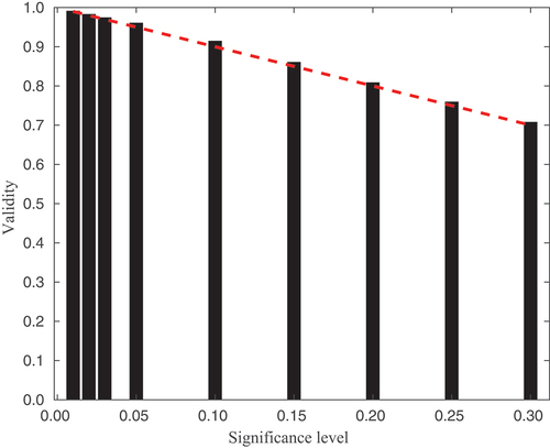
Figure 1 presents the validity of the 3-category Larch Casebearer model, for a range of significance levels, on the test data set. The theoretical relationship between validity and significance level is shown as the red dashed line. The empirical results closely match the theoretical level, thus showing that the CP framework is providing the guaranteed error rate according to the user-defined significance level.

Figure 1. The validity of the 3-category Larch Casebearer model on the test data compared to the selected significance level (black bars). The theoretical relationship between validity and significance level is shown as the red dashed line.

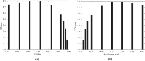
Figure 2(a) shows the trade-off between validity and efficiency for the 3-category Larch Casebearer model. It can be seen that when the validity is very high (close to 1.0), the efficiency decreases to a very low level of 0.15 – only 15% of the predictions. This demonstrates that the CP framework can achieve the high validity required, but due to the limitations of the underlying classifier, it can only do so by predicting many classes for each data sample. To maximize the efficiency of the classifier, the user must accept a validity of around 0.80–0.85 – that is, an error level of 0.15–0.20 (as can be seen in Figure 2(b)).

Figure 2. (a) Validity versus efficiency for the 3-category Larch Casebearer model. (b) Significance level versus efficiency for the 3-category Larch Casebearer model.

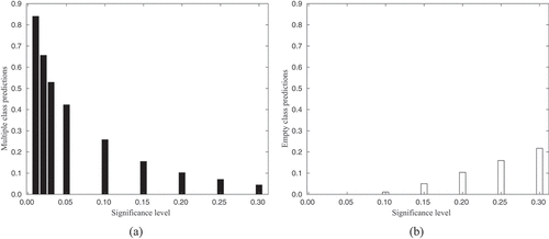
While the efficiency measures the number of prediction sets that contain only a single class, the CP framework can also return prediction sets that contain multiple classes, or no classes at all (the ‘empty’ prediction). Figure 3(a) presents the proportion of predictions that contain multiple classes, for different significance levels. As the significance level (the number of allowed errors) decreases to 0, the number of multiple class predictions rises steeply to more than 0.8. However, if we pick a significance level of 0.2 (which as seen in Figure 2(b) would provide the optimal efficiency level) the number of multiple class predictions is 0.10. At a significance level of 0.2, the number of empty class predictions is also 0.10.

Figure 3. (a) Proportion of multiple class predictions versus significance level for the 3-category Larch Casebearer model. (b) Proportion of empty classes versus significance level for the 3-category Larch Casebearer model.

Table 3 presents the number of multiple class predictions for the different class combinations for a significance level of 0.2. There are no multiple classes containing both Healthy and High Damage classes. Only the ‘neighbouring’ classes {Healthy, Low Damage} and {Low Damage, High Damage} have multiple-class predictions. Thus, the multiple-class predictions can be seen as identifying the ‘borderline’ cases between the two classes.

Table 3. Number of multiple class predictions for the 3-category Larch Casebearer model for a significance level of 0.2.

Predicted Classes	Proportion of predictions
{Healthy, Low Damage}	.0995
{Healthy, High Damage}	0
{Low Damage, High Damage}	.0029
{Healthy, Low Damage, High Damage}	0
All multiple class predictions	.1024

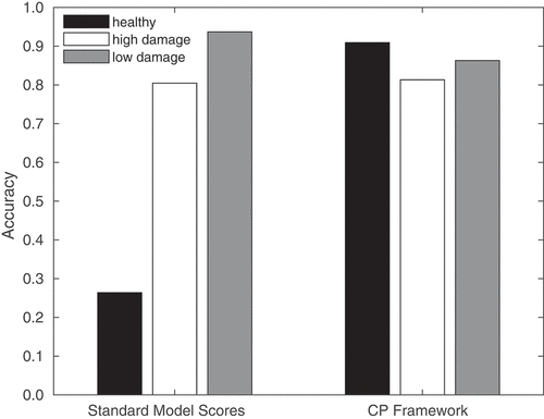
Finally, Figure 4 compares the per-class accuracy for the 3-category Larch Casebearer classifier using both the standard scoring approach and the CP framework. For this figure, the significance level of the CP framework was set to 0.15. It can be seen that the standard model has low accuracy on the small Healthy class, while the CP framework maintains high accuracy across all the classes. This demonstrates how the CP framework inherently handles class imbalance, without any oversampling or undersampling of the dataset required.

Figure 4. Per-class accuracy for the 3-category classifier using (left) standard scoring and (right) the CP framework (with a significance level of 0.15).

3.1. Two-class classifiers

Table 4 demonstrates the performance of the CP framework for the various 2-category Larch Casebearer models. For each, the significance level has been selected to optimize the efficiency of the model. The 3-category model has also been included for comparison. The results show that the 2-category models have a much higher validity and efficiency than the 3-category models achieves.

Table 4. Performance of the conformal predictors using the 2-category Larch Casebearer models. The 3-category model is also included for comparison.

Model	Validity	Efficiency	Empty	Multiple categories	Significance level
H_vs_LD_vs_HD (3 categories)	0.8081	0.7938	.1038	.1024	0.20
HLD_vs_HD	0.9038	0.9890	.0023	.0087	0.10
H_vs_LHD	0.8515	0.9913	.0073	.0013	0.15
H_vs_HD	0.9864	0.9901	.0099	0	0.01

3.2. Recognizing previously unseen classes

Table 5 demonstrates how the conformal predictor works when it is tested on a class of data that it has not been trained on. In this case, the LD class has been omitted from the training and the classifier only learns to differentiate between H and HD data. However, when the new LD category, as part of a test set containing all three classes, is introduced during testing into (H_vs_HD_with_LD) or as a single new category (H_vs_HD_withonly_LD, test set contains only the LD class) the model recognizes this and places or , respectively, of the LD category predictions in the ‘empty’ prediction category (bold numbers in Table 5) indicating that these examples are too different from the examples that the model has been trained and calibrated on. This is a large increase in the percentage of empty category labels compared to when the model only predicted categories for which the model was trained on, when only of classifications were placed in the empty category. This increase in empty category classifications indicates that some sort of domain shift or concept drift has taken place.

Table 5. Performance of the conformal predictor on a class of data that was previously unseen.

Model	Validity	Efficiency	Empty	Multiple categories	Significance level
H_vs_HD	0.9864	0.9901	.0099	0	0.01
H_vs_HD_with_LD^a	0.5089	0.9242	.0758	0	0.01
H_vs_HD_withonly_LD^b	-	0.9009	.0991	0	0.01

^aTest set contains classes: H, HD and LD.

^bTest set contains only class LD.

3.3. Comparison against traditional test set results

Table 6 compares the CP framework results with traditional test set results based only on the score-values of the deep learning model. In Table 6, since the efficiency is very high and few empty and multi-category predictions occur for these models, the difference in traditional performance statistics between the CP results and the corresponding results where the few empty and multi-category predictions were removed is negligible. However, it should also be noted that disregarding the CP significance level and make a single category prediction based on the CP -values, where the category with the largest -value determines to outcome, also works very well. However, the results of making predictions from the original Yolo model output (score) values without CP calibration are less satisfactory. This is shown with bold numbers in Table 6 where the SE for model HLD_vs_HD as well as SP for model H_vs_LHD are low as a result from significant over-training on the majority class in both cases (HLD and LHD, respectively) as can be expected. Mondrian CP, on the other hand, gracefully handles category imbalances without explicit over- or under-sampling or category weighting as a result of the recalibration procedure employed to calculate the CP -values that forms the basis for CP category prediction (Alvarsson et al. 2021; Vovk, Gammerman, and Shafer 2005).

Table 6. Traditional test set results from binary conformal prediction models^a.

Modelb	Significance level	Sensitivity	Specificity	BA	F1-score	MCC	Kappa	Precision	ROC curve	Commentc
HLD_vs_HD	0.10	0.9198	.8966	0.9082	0.7907	0.7402	.7278	.6934	0.9082
HLD_vs_HD	0.10	0.9263	.8997	0.913	0.7978	0.7496	.7373	.7006	0.9130	no_mlt_cat
HLD_vs_HD		0.7660	.9613	0.8637	0.7989	0.7514	.7503	.8347	0.8637	score-values
HLD_vs_HD		0.9165	.8959	0.9062	0.7885	0.7370	.7247	.6918	0.9062	max_-value
H_vs_LHD	0.15	0.8565	.8731	0.8648	0.9188	0.4406	.3616	.9908	0.8648
H_vs_LHD	0.15	0.8566	.8742	0.8654	0.9189	0.4415	.3623	.9909	0.8654	no_mlt_cat
H_vs_LHD		0.9773	.5171	0.7472	0.9737	0.5243	.5232	.9702	0.7472	score-values
H_vs_LHD		0.8542	.8711	0.8627	0.9174	0.4357	.3559	.9907	0.8627	max_-value
H_vs_HD	0.01	0.9963	.9961	0.9962	0.9976	0.9893	.9893	.9989	0.9962
H_vs_HD	0.01	0.9963	.9961	0.9962	0.9976	0.9893	.9893	.9989	0.9962	no_mlt_cat
H_vs_HD		0.9942	.9848	0.9895	0.9949	0.9772	.9772	.9956	0.9895	score-values
H_vs_HD		0.9927	.9937	0.9932	0.9954	0.9799	.9798	.9982	0.9932	max_-value

^aAbbreviations: Significance level = CP significance level, BA = Balanced accuracy, MCC = Matthews correlation coefficient, Kappa coefficient = Cohen’s kappa coefficient, ROC = Receiver operating characteristic curve.

^bModel nomenclature catA_vs_catB: catA and catB associated with (TN,FP,SP) and (FN,TP,SE), respectively.

^cno_mlt_cat = no multi or empty predictions included in the results, score-values = original score values from the Yolo model were used for assigning the class, max_-value = maximum CP -value was used for assigning the class.

4. Discussion

Our investigation related to damages caused by the Larch Casebearer indicates advantages of using a combination of a confidence predictor framework, in this case conformal prediction, in combination with a deep learning architecture. Compared with the traditional approach using only the corresponding deep learning architecture, the advantages include the mathematically proven error rate levels from the model for each class where the user may decide at which level, i.e., error rate percentage, the model should operate in order to deliver useful predictions to the user for the decision to be taken on the basis of these predictions.

The conformal prediction framework also determines the applicability domain of the model, i.e., where the model can provide reliable predictions, as an intrinisic property and part of the model development. Thus, predictions containing more than one label, e.g., {H,LD}, {H,HD}, {LD,HD}, {H,LD,HD} for the 3-class investigation and both for the 2-class investigation, indicate that the input image features provided to the model do not contain sufficient information to allow for a single-label outcome at the error level set by the user and that more information needs to be provided in order to resolve this. Alternatively, the uses may decide to increase the error rate and possibly resolve some of the multi-label predictions.

The occurrence of many {empty} predictions, i.e., where no label can be assigned to an example at the error level set by the user, indicate that these examples are different from the examples on which the model has been trained and out-of-applicability-domain so that the model cannot provide reliable predictions. Furthermore, as shown in Table 6, the framework gracefully handles class imbalances without explicit over- or under-sampling or category weighting which may be of crucial importance in cases of highly imbalanced datasets particularly when the minority class(es) are the one(s) of importance.

The framework is also capable of identifying domain shifts or concept drift exemplified in Table 5 for the ‘H_vs_HD’ model when the introduction of the new LD category caused an increase the {empty} predictions indicating that something new and different has been predicted or that the relationship between input and output, on which the model was built, has changed. In either case, this observation would trigger a closer investigation of these different/new examples and the new LD class would then be identified.

5. Conclusion

It is of considerable importance to monitor forests health and to identify biodiversity hazards to maintain environmental balance as well as sustainable forests. Forests cover large areas of land, sometimes very inaccessible for closer investigations, and images captured from the air, e.g., by drones, may provide essential information for the determination of the health of forests. By using the combination of a confidence predictor framework in combination with a deep learning architecture successful forecasting models can be derived that are able not only to predict the current types of diseases used to develop the model but also provide indication of new, unseen, types or degrees of disease. The user of the models is also, at the same time, provided with reliable predictions and a well-established applicability domain for the model where such reliable predictions can and cannot be expected. The framework also gives indication of when insufficient information has been provided at the level of accuracy (reliability) need by the user to make subsequent decisions based on the model predictions.

Disclosure statement

No potential conflict of interest was reported by the author(s).

Data availability statement

The data used in this study are publicly available at these locations: https://skogsdatalabbet.se/delning_av_ai_larksackmal/and https://lila.science/datasets/forest-damages-larch-casebearer/

Additional information

Funding

This work was supported by the Swedish Research Council [grant number 2018-03807].

References

- Alvarsson, J., S. Arvidsson McShane, U. Norinder, and O. Spjuth. 2021. “Predicting with Confidence: Using Conformal Prediction in Drug Discovery.” Journal of Pharmaceutical Sciences 110 (1): 42–49. https://doi.org/10.1016/j.xphs.2020.09.055.
- Angelopoulos, A. N., S. Bates, M. I. Jordan, and J. Malik. 2021. “Uncertainty Sets for Image Classifiers Using Conformal Prediction.” OpenReview.net. https://openreview.net/forum?id=eNdiU_DbM9.
- Barmpoutis, P., V. Kamperidou, and T. Stathaki. 2020. “Estimation of Extent of Trees and Biomass Infestation of the Suburban Forest of Thessaloniki (Seich Sou) Using UAV Imagery and Combining R-CNNs and Multichannel Texture Analysis.” 11433:1. https://doi.org/10.1117/12.2556378.
- Deng, X., Z. Tong, Y. Lan, and Z. Huang. 2020. “Detection and Location of Dead Trees with Pine Wilt Disease Based on Deep Learning and UAV Remote Sensing.” AgriEngineering 2 (2): 294–307. https://doi.org/10.3390/agriengineering2020019.
- Diez, Y., S. Kentsch, M. Fukuda, M. Larry Lopez Caceres, K. Moritake, and M. Cabezas. 2021. “Deep Learning in Forestry Using UAV-Acquired RGB Data: A Practical Review.” Remote Sensing 13 (14): 2837. https://doi.org/10.3390/rs13142837.
- Fisch, A., T. Schuster, T. Jaakkola, and R. Barzilay. 2022. “Conformal Prediction Sets with Limited False Positive.” 162 (3): 6514–6532 PMLR. https://proceedings.mlr.press/v162/fisch22a.html.
- Hamedianfar, A., C. Mohamedou, A. Kangas, and J. Vauhkonen. 2022. “Deep Learning for Forest Inventory and Planning: A Critical Review on the Remote Sensing Approaches so Far and Prospects for Further Applications.” Forestry: An International Journal of Forest Research 95 (4): 451–465. https://doi.org/10.1093/forestry/cpac002.
- Hernández-Hernández, S., S. Vishwakarma, and P. Ballester. 2022. “Conformal Prediction of Small-Molecule Drug Resistance in Cancer Cell Lines.” 179 (3): 92–108 PMLR. https://proceedings.mlr.press/v179/hernandez-hernandez22a.html.
- Hoeser, T., F. Bachofer, and C. Kuenzer. 2020. “Object Detection and Image Segmentation with Deep Learning on Earth Observation Data: A Review—Part II: Applications.” Remote Sensing 12 (18): 12. https://doi.org/10.3390/rs12183053.
- Hoeser, T., and C. Kuenzer. 2020. “Object Detection and Image Segmentation with Deep Learning on Earth Observation Data: A Review-Part I: Evolution and Recent Trends.” Remote Sensing 12 (10): 12. https://doi.org/10.3390/rs12101667.
- Hossain, F. M. A., Y. M. Zhang, and M. Akter Tonima. 2020. “Forest Fire Flame and Smoke Detection from UAV-Captured Images Using Fire-Specific Color Features and Multi-Color Space Local Binary Pattern.” Journal of Unmanned Vehicle Systems 8 (4): 285–309. https://doi.org/10.1139/juvs-2020-0009.
- Jocher, G., A. Chaurasia, A. Stoken, J. Borovec, Y. K. NanoCode012, K. Michael. 2022. “Ultralytics/Yolov5: V7.0 - YOLOv5 SOTA Realtime Instance Segmentation.” 11. https://doi.org/10.5281/zenodo.7347926.
- Johnson, J. M., and T. M. Khoshgoftaar. 2019. “Survey on Deep Learning with Class Imbalance.” Journal of Big Data 6 (1): 27. https://doi.org/10.1186/s40537-019-0192-5.
- Kattenborn, T., J. Leitloff, F. Schiefer, and S. Hinz. 2021. “Review on Convolutional Neural Networks (CNN) in Vegetation Remote Sensing.” ISPRS Journal of Photogrammetry and Remote Sensing 173:24–49. https://doi.org/10.1016/j.isprsjprs.2020.12.010.
- Laxhammar, R., and G. Falkman. 2010. Conformal Prediction for Distribution-Independent Anomaly Detection in Streaming Vessel Data. Association for Computing Machinery 47–55. https://doi.org/10.1145/1833280.1833287.
- LeCun, Y., Y. Bengio, and G. Hinton. 2015. “Deep Learning.” Nature 521 (7553): 436–444. https://doi.org/10.1038/nature14539.
- Minařík, R., J. Langhammer, and T. Lendzioch. 2021. “Detection of Bark Beetle Disturbance at Tree Level Using UAS Multispectral Imagery and Deep Learning.” Remote Sensing 13 (23): 4768. https://doi.org/10.3390/rs13234768.
- Nguyen, H. T., M. Larry Lopez Caceres, K. Moritake, S. Kentsch, H. Shu, and Y. Diez. 2021. “Individual Sick Fir Tree (Abies Mariesii) Identification in Insect Infested Forests by Means of UAV Images and Deep Learning.” Remote Sensing 13 (2): 260. https://doi.org/10.3390/rs13020260.
- Norinder, U., and S. Boyer. 2017. “Binary Classification of Imbalanced Datasets Using Conformal Prediction.” Journal of Molecular Graphics and Modelling 72:256–265. https://doi.org/10.1016/j.jmgm.2017.01.008.
- Norinder, U., L. Carlsson, S. Boyer, and M. Eklund. 2014. “Introducing Conformal Prediction in Predictive Modeling. A Transparent and Flexible Alternative to Applicability Domain Determination.” Journal of Chemical Information and Modeling 54 (6): 1596–1603. https://doi.org/10.1021/ci5001168.
- Olsson, H., K. Kartasalo, N. Mulliqi, M. Capuccini, P. Ruusuvuori, H. Samaratunga, B. Delahunt, et al. 2022. “Estimating Diagnostic Uncertainty in Artificial Intelligence Assisted Pathology Using Conformal Prediction.” Nature Communications 13 (1): 7761. https://doi.org/10.1038/s41467-022-34945-8.
- Radogoshi, H. 2021. “Using Artificial Intelligence to Map and Follow Up Damage Caused by the Larch Casebearer.” https://skogsdatalabbet.se/delning_av_ai_larksackmal/.
- Reichstein, M., G. Camps-Valls, B. Stevens, M. Jung, J. Denzler, N. Carvalhais, and Prabhat, P. 2019. “Deep Learning and Process Understanding for Data-Driven Earth System Science.” Nature 566 (7743): 195–204. https://doi.org/10.1038/s41586-019-0912-1.
- Russakovsky, O., J. Deng, S. Hao, J. Krause, S. Satheesh, M. Sean, Z. Huang, et al. 2015. “ImageNet Large Scale Visual Recognition Challenge.” International Journal of Computer Vision 115 (3): 211–252. https://doi.org/10.1007/s11263-015-0816-y.
- Schmidhuber, J. 2015. “Deep Learning in Neural Networks: An Overview.” Neural Networks 61:85–117. https://doi.org/10.1016/j.neunet.2014.09.003.
- Shi, W., M. Zhang, R. Zhang, S. Chen, and Z. Zhan. 2020. “Change Detection Based on Artificial Intelligence: State-Of-The-Art and Challenges.” Remote Sensing 12 (10): 12. https://doi.org/10.3390/rs12101688.
- Szeliski, R. 2011. Computer Vision Algorithms and Applications. Springer London. https://doi.org/10.1007/978-1-84882-935-0.
- Vazquez, J., and J. C. Facelli. 2022. “Conformal Prediction in Clinical Medical Sciences.” Journal of Healthcare Informatics Research 6 (3): 241–252. https://doi.org/10.1007/s41666-021-00113-8.
- Vovk, V., A. Gammerman, and G. Shafer. 2005. Algorithmic Learning in a Random World. 1st ed. New York, NY: Springer.
- Zhang, R., L. Qing, K. Duan, S. You, T. Zhang, K. Liu, and Y. Gan. 2020. “Precise Classification of Forest Species Based on Multi-Source Remote-Sensing Images.” Applied Ecology and Environmental Research 18 (2): 3659–3681. https://doi.org/10.15666/aeer/1802_36593681.
- Zhao, Y., M. Jiale, L. Xiaohui, and J. Zhang. 2018. “Saliency Detection and Deep Learning-Based Wildfire Identification in UAV Imagery.” Sensors 18 (3): 18. https://doi.org/10.3390/s18030712.
- Zhu, X. X., D. Tuia, L. Mou, G.-S. Xia, L. Zhang, X. Feng, and F. Fraundorfer. 2017. “Deep Learning in Remote Sensing: A Comprehensive Review and List of Resources.” IEEE Geoscience and Remote Sensing Magazine 5 (4): 8–36. https://doi.org/10.1109/MGRS.2017.2762307.