Ecological data prediction and visualization system

Abstract

Temporal patterns in ecological data can be visualized and communicated effectively through graphical means. The aim of this study was to develop a data prediction and visualization system based on historical data and thematic map technology to visualize forecast temporal ecological changes. The visualization system consists of prediction and data visualization modules. The prediction module is developed using a hybrid evolutionary algorithm (HEA) to classify and predict noisy ecological data. The visualization module is developed using Dotnet Framework 2.0 to implement thematic cartography for volume visualization. The visualization system is evaluated by its capability in representing the output data on a map, and by predicting the abundance of Chlorophyta based on other water quality parameters. Rules for predicting Chlorophyta abundance had a success rate of almost 90%. The integration of computational data mining using HEA and visualization using thematic maps promises practical solutions and better techniques for forecasting temporal ecological changes, especially when data sets have complex relationships without clear distinction between various variables.

Keywords:

• data visualization
• ecological system
• prediction
• water quality
• HEA

Introduction

Data visualization is important as it enables the communication of information clearly and effectively through graphical means. It is useful for analysing and exploring the huge amounts of ecological data that are an immense source of important information for research and decision making (MacEachren & Kraak 2001). Ecological data contain an array of distinctive features making them valuable, yet challenging to visualize (Helly et al. 1999). The goal of ecological visualization is to combine the strengths of human vision, creativity and general knowledge with the storage capacity and the computational power of modern computers in order to explore large geospatial data sets. One way of undertaking this task is by presenting a multitude of graphic representations of the data to the user, which allows him or her to interact with the data and change the views in order to gain insight and to draw conclusions quickly (Keim et al. 2005). It is also important to be able to visualize the relationships and patterns discovered from complex ecological data.

Effective visual data-mining tools are required to display multivariate and spatiotemporal ecological data to easily perceive patterns and relationships. Common visualization techniques for multivariate data are geometric, glyph or icon-based pixel-oriented and hierarchical methods (Keim & Kriegel 1996; Schroeder 2005). Spatiotemporal data require a map display to visualize the spatial attributes of the data in order to reveal, analyse and understand patterns (Andrienko et al. 2003, 2005). Thematic maps are an effective method of data visualization and are widely used for the representation of ecological data (Few 2014). A thematic map is designed with a specific theme and topic. It does not contain any physical features such as rivers, roads or subdivisions; it usually uses city locations, country maps, rivers and other geographical locations as its base maps.

Several computational methods such as the hybrid evolutionary algorithm (HEA) and artificial neural network (ANN) have been developed in different areas including machine learning and data mining, which can analyse large data volumes and automatically extract knowledge. HEAs and ANNs have been successfully applied to unravel and predict complex and non-linear ecological data, e.g. algal population dynamics for eutrophication modelling and lake management (Melesse et al. 2008; Welk et al. 2008). Algae respond to a wide range of pollutants and are thus a good indicator of eutrophication. The temporal dynamics of algal communities are influenced by a complex array of biotic and abiotic factors operating through both direct and indirect pathways (Carrillo et al. 1995). ANN models are highly flexible functions that can be used to model non-linear relationships. HEAs can also be used to model non-linear relationships. However, the HEA has the advantage over ANN that it uses genetic programming (GP) to generate the structure of the rule set, and a genetic algorithm (GA) for parameter optimization.

Data-mining methods have limited pattern-interpretation abilities. This limitation can be overcome using exploratory data analysis (also known as visual data mining), which aims at visually analysing data and gaining new insights (Tukey 1977). This is the opposite of computational data-mining techniques which use algorithms to detect patterns in the data. Computational methods can be complemented by visual approaches, however. The integration of both approaches to combine their advantages promises further advances in the exploration of data for knowledge discovery (MacEachren & Kraak 2001). This has been demonstrated using Kohonen's self-organizing maps (SOMs), a form of supervised ANN for detecting clusters in a data set (Koussoulakou & Kraak 1992; Andrienko & Andrienko 2004; Guo et al. 2005). A detailed explanation of SOMs can be found in Guo et al. (2005). Here, an SOM is linked with a map, which illustrates the integration of a computational data-mining technique into a visualization system. This allows the exploration of large geospatial data sets. The visual information load is reduced by automatically clustering the data and displaying summary information while details are still available on demand. SOMs have been successfully applied to unravelling algal population dynamics (Sorayya et al. 2011).

Even though ANN models are able to make perfect predictions and are recognized as a powerful technique, they are considered to be ‘black box’ in nature. The HEA approach can overcome the current limitations of the ANN approach. The HEA allows discovery of predictive rule sets in complex ecological data. The HEA as used by Cao et al. (2006) is adopted in this study to discover predictive rules over the black-box approach of ANNs. The HEA evolved from the evolutionary algorithm, with additional features of parameter optimization. The HEA model optimizes variable selection using a general GA approach. Its crossover operator is based on the non-convex linear combination of multiple parents during the recombination of the population for parameter optimization (Cao et al. 2006). The main characteristic of the HEA is its ability to solve problems of complex and noisy environments, under imprecision, uncertainty and vagueness.

The thematic map method is adopted in this study to visualize the predictive rules from HEA. Thematic maps have been used successfully in many areas of ecological informatics research, such as coastal management, detection of toxic dinoflagellates and marine eutrophication (Macleod & Congalton 1998; Klemas 2009). Thematic maps have been generated by integrating satellite data with in situ water quality measurements such as suspended matter concentration, chlorophyll concentration, turbidity, algal bloom indicators and sea surface temperature for European users to monitor the marine environment (Marine and Coastal Environment Information Services n.d.).

A choropleth map represents quantitative data such as percentage, density and average values of an event in a geographical area using colour representation. Different colours represent a certain range of data (Briney n.d.). In the present study, a choropleth map is linked to rule sets generated from the HEA. This is designed to predict the Chlorophyta abundance, and integrate the computational data-mining technique of HEA into a visualization system. Data from 2001 to 2006 on the Putrajaya Wetlands were used to evaluate the developed system. The HEA was applied to discover the best rules for predicting Chlorophyta abundance in relation to water quality parameters. Chlorophyta are affected by water conditions such as dissolved oxygen, water temperature, pH, salinity and turbidity. In addition, Chlorophyta require nutrients such as nitrates, phosphates and silicates for their survival and growth. All these factors determine the spatiotemporal abundance of Chlorophyta. Common genera of Chlorophyta in Putrajaya Lake and Wetlands include Ankistrodesmus, Chlorella, Closteriopsis, Cosmarium, Crucigenia, Pediastrum, Scenedesmus, Staurastrum and Tetrahedron (Perbadanan Putrajaya n.d.). Staurastrum is the most dominant genus in terms of distribution in Putrajaya Lake and its peripheral wetlands (Portal Rasmi, Perbadanan Putrajaya, n.d.). Blooming of Staurastrum leads to degradation of water quality and water pollution. The presence of Staurastrum is usually accompanied by foul odour, bad taste and toxification of an aquatic ecosystem (Saravi et al. 2008).

The objective of this study was to develop a visualization system that is integrated with data-mining capabilities. The ultimate aim is to provide a tool that will be useful for ecosystem monitoring. This article is organized as follows. The next section discusses the methodology, which includes details of the study area, data collection, analyses and preparation. Then, the prediction and visualization system development process are described. The results and discussion are presented, and the final section summarizes the conclusions of this study.

Methods

Study site and data collection

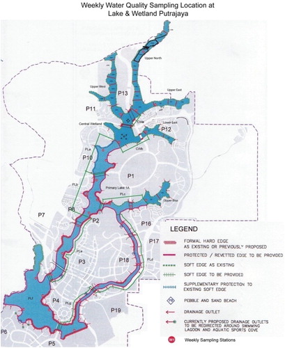
Putrajaya Lake and Wetlands were created by inundation of 400 ha of the valleys of Sungai Chuau and Sungai Bisa. The Putrajaya Wetlands were designed as a multicell, multistage system with flood retention capability. The Putrajaya Wetlands comprise six arms, as shown in Figure 1 (Malek et al. 2009): Central Wetland, Lower East Wetland, Upper Bisa Wetland, Upper East Wetland, Upper North Wetland and Upper West Wetland (Perbadanan Putrajaya n.d.).

Figure 1. Map of Putrajaya Lake and Wetlands, showing water quality sampling stations (Malek et al. 2009).

Data used to generate rule sets to predict Chlorophyta abundance were collected biweekly from 2001 to 2006 from various sampling stations at Putrajaya Lake and Wetlands. Water sampling for water quality and diatom abundance analyses was carried out according to the American Public Health Association (Eaton et al. 1995) and World Health Organization (WHO 1987). Water samples for algae identification were collected using plankton nets with a mesh size of about 30 µm. Smaller mesh-size plankton nets were not used because of problems of clogging and reduced water flow during the transfer of water to vials for subsequent analysis (Bellinger & Sigee 2010). Each water sample for algae analysis was gathered from several scoops of the site water to reduce the chances of omitting smaller Chlorophyta from the sample. Algae were preserved by adding several drops of 4% formaldehyde to the water samples, which were subsequently kept in 50 ml vials. Algae were identified using an ordinary light microscope. Identification of algae genera was based on literature such as Wehr and Sheath (2003). Algae abundance was calculated using the sedimentation technique and procedure described by Evans (1972).

Data preparation and rule set generation

Rule sets for Chlorophyta abundance were generated for each area of the Putrajaya Wetlands (Central Wetland, Lower East Wetland, Upper Bisa Wetland, Upper West Wetland, Upper East Wetland and Upper North Wetland). The data were divided arbitrarily into two sets (data sets A and B) for each wetland in order to minimize bias in the generated results. Data from data set A were used for training, and data set B for testing the rule set generated. Parameters used as input variables were rainfall, wind speed, sunshine, temperature, pH, dissolved oxygen, Secchi depth, turbidity, conductivity, total phosphorus, NH₃-N, NO₃-N, biochemical oxygen demand, chemical oxygen demand and total suspended solids. Summary characteristics of the data used in this study are given in Table 1.

Table 1. Mean limnological properties of Putrajaya Wetlands based on data collected from 2001 to 2006.

Parameter	Minimum value	Maximum value	Mean	Standard deviation
Rainfall (mm)	0.0	71.8	0.4	13.63488
Wind speed (m/s)	0.23	1.73	0.7	0.23655
Sunshine (h)	0.00	11.20	6.29	2.559912
Temperature (°C)	25.77	35.28	30.22	1.766512
pH	4.26	8.61	7.14	0.515269
Dissolved oxygen (mg/l)	3.27	8.50	6.43	0.996298
Secchi depth (m)	0.05	2.00	0.60	0.303146
Turbidity (NTU)	0.00	527.00	35.24	44.984791
Conductivity (μS/cm)	37	228	98.54	40.375525
Total PO4 (mg/l)	0.00	1.13	0.04	0.112034
NH3-N (mg/l)	0.00	2.63	0.14	0.326953
NO3-N (mg/l)	0.00	5.17	1.42	1.114293
Total Chlorophyta (cells/ml)	1	510	37	50.871022

Before HEA model development, data output in the form of Chlorophyta abundance was classified using statistical distribution into low (< 70 cells/ml), medium (< 100 cells/ml) and high (> 100 cells/ml). The trichotomized values of Chlorophyta were used to enable prediction and visualization of Chlorophyta based on these levels.

Hybrid evolutionary algorithm model

The HEA was used in this study to generate the best rule set for prediction of Chlorophyta abundance. The HEA uses GP to create and optimize the formation of rule sets and a GA is used to optimize the parameters of a rule set in a typical GP. Computer programs can be depicted as parse trees, where a branch node depicts an element from a function set (arithmetic operators, logic operators and elementary functions of at least one argument) and a leaf node depicts an element from a terminal set (variables, constants and functions of no arguments). These symbolic programs are later assessed using ‘fitness cases’. Fitter programs are chosen for recombination to form the next generation by means of genetic operators, e.g. crossover and mutation. This process is iterated for successive generations until the termination criterion is fulfilled. A general GA was applied for parameter optimization of the random parameters in the rule set. One-hundred runs were conducted independently for each data set. For simplicity, the maximal rule size was set to be single rule.

All the experiments were performed using the HEA for rule set generation on a University of Malaya high-performance supercomputer (Altix SGI 1300) using the programming language C. The HEA uses GP to generate and optimize the structure of rule sets and a GA to optimize the parameters of a rule set. GP is an extension of GAs, in which the genetic population consists of varying sizes and shapes. These modules are subsequently evaluated by means of fitness cases. Fitter programs are selected for recombination to create the next generation using genetic operators, such as crossover and mutation. This step is iterated for consecutive generations until the termination criterion of the run has been satisfied. A general GA is used to optimize the random parameters in the rule set; 50 out of 10,000 best rules (100 generations out of 100 chromosomes) will be selected based on its accuracy (Cao et al. 2006).

System development

The system was developed in two parts: (i) integration of the HEA for rule set generation to predict Chlorophyta abundance; and (ii) thematic map development for visualization of Chlorophyta abundance over time.

Prediction module

The prediction module flowchart is shown in Figure 2. The module requires rules generated by the HEA and ecological data to be visualized. The uploaded rules are analysed by extracting each element from the rule set, such as the arithmetic operators, logical operators, variables and constants.

Figure 2. Prediction module flowchart. HEA = hybrid evolutionary algorithm.

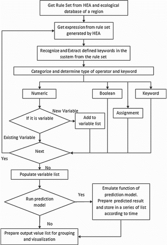
After all the expressions have been extracted from the rule sets, the variable list is populated. The user is given the option to choose the output variable to be predicted. The prediction module function uses this information to calculate the predicted output. This study illustrates the prediction of Chlorophyta abundance output in terms of threshold categories of ‘low', ‘medium' and ‘high’; this is stored in a temporary file before being displayed over the constructed thematic map using the visualization module.

The accuracy of the rules is measured based on sensitivity, which statistically measures the performance of a binary classification test. Sensitivity, also called the true-positive rate, is used to measure the proportion of actual positives predicted that are correctly identified. The rule accuracy and prediction model are described in the Results and Discussion section.

Visualization module

The data visualization system was developed using Dotnet Framework 2.0. The data visualization approach in this study combines thematic cartography with volume visualization. Volume visualization is a set of techniques which present and show an object without mathematical representation (Hesselink & Delmarcelle 1994). The rules generated using the HEA are integrated with the thematic map to visualize Chlorophyta abundance over time. A choropleth map was adopted in this study to visualize Chlorophyta abundance at different levels that correspond to colours. Using volume visualization, different colours are used to represent the different range of Chlorophyta abundance: ‘low', ‘medium' and ‘high'. Figure 3 illustrates the flowchart of the visualization module, where the output of a predicted variable from the ecological data is displayed and iterated over time on the uploaded map for each selected region on the map. The regions represent different areas on the map.

Figure 3. Visualization module flowchart.

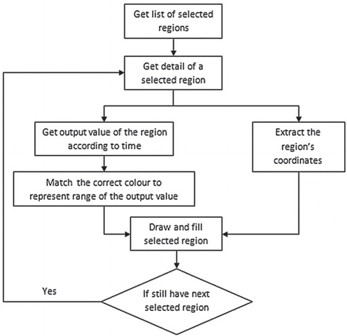
In this study, regions are referred to as wetlands. The thematic map used to evaluate the visualization system is made up of six different wetlands or regions. The coordinates of each selected region (wetland) are mapped on to the thematic map. The selected regions (wetlands) on the map will be automatically assigned different colours based on their coordinates to differentiate each region. Ecological data for each region (wetland) are linked with a timeline, and the date format and data are assigned automatically. The predicted output variable is displayed with varying colours on the selected region of the thematic map over time. For example, the colour red is associated with high abundance, green with medium abundance and yellow with low abundance. Options are available to the user to alter the colour display settings. The colour can be multicontrasted, with a natural colour shifting gradually from green for low output values to red for high output values. The entire sequence of steps and processes is repeated for the remaining selected regions for a selected time-frame. Upon completion, the result of the entire selected area of the map is displayed for visualization. The technique used is based on Shanbhag et al. (2005), who modified choropleth maps to display temporal attribute data. Each area on the map is not represented uniformly but partitioned into several regions, each representing temporal trends in the area that could be detected by observing the variation (e.g. brightness, colour) of the different regions of the area.

System interface

Interaction is paramount in ecological data visualization, especially for visual exploration. In the following, the user interface for the visual data-mining prototype developed in this study is illustrated.

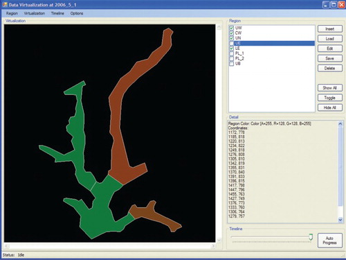
The graphical user interface of the visualization system illustrated in Figure 4 has four main menu options on the main toolbar, labelled Region, Visualization, Timeline and Options. The Region menu is further subdivided into submenu commands, which consist of Insert, Load, Edit, Save, Delete and Exit. The Insert menu option is used to create a new map profile with the extension *.rd, which contains the coordinates, rules sets and data sets of the different regions of the map. The Load menu option consists of two submenus: Append and Replace options. Append allows the user to append a new region (wetland) to the existing map, while Replace allows the user to delete the selected region from the current map and replace it with a new region. The Edit option allows the user to modify the region coordinates, rule sets and data sets on a specific region on the map. The Delete option contains two suboptions which allow the user to delete either only the selected region or the whole map profile. The Visualization menu bar contains controls for thematic map representation. The Timeline menu bar contains controls for the running timeline for data visualization. The Options menu bar contains the basic main functions in the data visualization system.

Figure 4. Graphical user interface of the system.

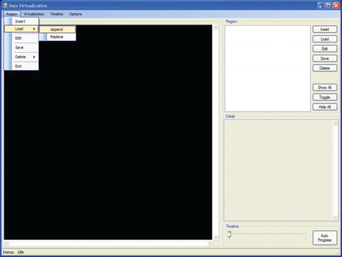
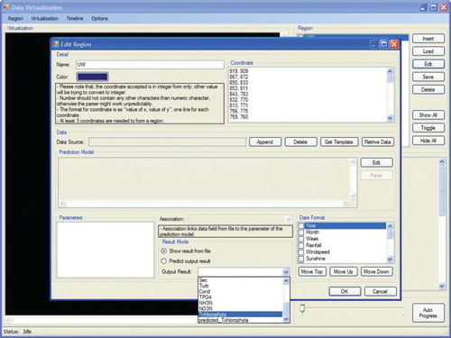
A map is made up of a number of regions or areas. Once a map has been uploaded, a vertical check box listing the available regions or areas on the map will be displayed. The window area consists of eight vertical menu buttons to manipulate the regions or areas on the map. The Insert button allows the user to add new regions to the current map. The Load button allows the user to load a certain region data into the current map, as shown in Figure 5. Edit, Save and Delete are used to modify, store and delete a particular region. The subsequent step is shown in Figure 6. Figure 7 illustrates a dialogue box when the Options menu is selected. The dialogue box is used to adjust colour hue and intensity for representing the Chlorophyta abundance intensity from low (green colour) to high (red colour). Colours representing the gradual change from low abundance (green) to high (red) can be assigned either manually in the designated text-box area or automatically by the system. Options are also available to resize the map and set the map boundary for each region in terms of colour and width. Frequency and Number of Date Field, under the heading Timeline, are used to set the frequency of data displayed on the visualization map. Figure 8 illustrates a dialogue box when the Insert submenu option is selected from the Region menu. This dialogue box is used to attach data on the selected region to be visualized. The dialogue box displays the region name, coordinates of the region and colour of the region on the map. The text area labelled Prediction Model allows insertion of the rule sets generated by the HEA for a particular region. However, before integration of the rules into the thematic map the rules need to be selected, and then only the prediction output can be displayed.

Figure 5. Example of visualization interface.

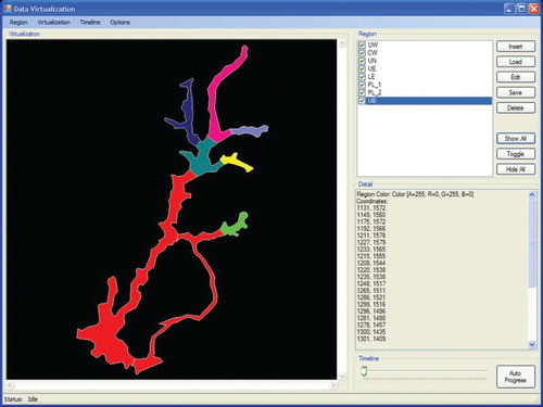
Figure 6. Scenario of integrating rule sets generated from the hybrid evolutionary algorithm into a thematic map after uploading the map profile.

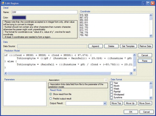
Figure 7. Dialogue box when the Options menu is selected on the main toolbar.

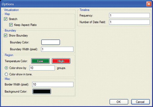
Figure 8. Select output variable.

Results and discussion

This section covers the rules generated from the HEA and visualization of the predicted data based on those rules. The visualization system was evaluated using the data from Putrajaya Wetlands. These data were used to extract rules to predict Chlorophyta abundance in relation to water quality parameters using the HEA. The percentage of accuracy or true-positive value was calculated for each part of the wetlands. Table 2 describes HEA rules generated for the data visualization system from all six parts of the wetlands from 2001 to 2006. Each section contains one best rule set and the rule sets are divided into two branches, called the IF branch and the ELSE branch.

Table 2. Results of rule sets and accuracy generated using the hybrid evolutionary algorithm.

	Rule sets
Putrajaya Wetlands	Condition statement (IF)	(THEN)	(ELSE)	Accuracy (%)
Central Wetlands (CW)	((((Sunshine*Sunshine)> =79.010)AND(Cond> =52.825))AND ((DO*DO)> =49.065))	Tchlorophyta= (exp(NO3N)*50.846)	Tchlorophyta= (((NO3N/exp(NO3N)) *45.347)− (((NO3N*(−10.179))/(149.747-Cond))*51.734))	91.14
Lower East Wetlands (LE)	(((158.687/Rainfall) >90.737)OR(((Cond+ Sunshine)> =74.965)OR((Cond> 16.596)AND(Rainfall >10.321))))	Tchlorophyta=(NH3N+ (Temp+(−1.215)))	Tchlorophyta=((((Turb +234.147) +(−1.610)) +(−1.610)) +(−1.304))	93.59
Upper Bisa Wetlands (UB)	((Turb*428.965)> 428.965)	Tchlorophyta=((85.916/ ((41.978/NO3N)-Cond))+28.769)	Tchlorophyta= 226.054	96.55
Upper East Wetlands (UE)	((Sunshine<=9.583) AND((Rainfall> =8.487)OR(Rainfall< =6.549)))	Tchlorophyta= (exp(exp(Windspeed)) +(exp(exp(Windspeed)) +23.026))	Tchlorophyta= (Turb+236.425)	96.97
Upper North Wetlands (UN)	(((exp(NO3N)/TPO4) >19.590)OR((Sunshine/ TPO4)<=86.085))	Tchlorophyta= ((ln(|ln(|Turb|)|)+ 5.129)+(Cond/(exp(pH)/ (Cond-(-144.302)))))	Tchlorophyta= (((32.515/NO3N)+ 121.739)+Turb)	84.96
Upper West Wetlands (UW)	((((Cond+NH3N)+ NH3N)+(Cond+ NH3N))<97.474)	Tchlorophyta=(((pH/ (Sunshine-Rainfall))+23.026)+ ((Sunshine*pH)/ exp(Cond)))	Tchlorophyta=(Rainfall+ (((Sunshine*pH)/ (Cond +(-80.792))) +23.212))	95.12

All the parameters detected by the HEA rules are extracted and populated into the text area labelled Parameter. The text area displays all the parameters contained inside the rule sets. The user has to link the parameters of rule sets with parameters from the ecological data sets by selecting parameters from the dropdown menu labelled Associate. This is to ensure that any mismatches in labelling of the parameters in the data file and rules are resolved before the prediction can take place by selecting the radio button option to predict the output results. The visualization module can be used without the prediction module for any other parameters from the ecological data set file.

Equidistant projections were used for this study to generate a thematic map of Putrajaya Wetlands for the visualization system. The thematic map for the visualization system as shown in Figure 9(B) was generated using tracing methods based on an existing map of Putrajaya Wetlands as shown in Figure 9(A). The thematic map along with geographical coordinates of each region (wetland) on the map was uploaded to the system. Once the map and the coordinates had been uploaded, the map was resized according to the global minimum and maximum values. Figure 10 illustrates the visualization results of Chlorophyta abundance prediction over time. The wetlands coloured green show a low abundance of Chlorophyta, and the wetlands coloured red show a high abundance of Chlorophyta. The user can choose whether to hide one or more regions, show all the regions or hide all the regions, and can also toggle the current selection. The timeline used to display the prediction of Chlorophyta abundance over time depends on the time range of the data set uploaded to the system.

Figure 9. (a) Putrajaya Wetlands; (b) thematic map of Putrajaya Wetlands.

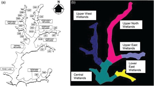
Figure 10. Visualization of Chlorophyta abundance over time.

The ecological visual data-mining prototype integrates the visual capabilities of the choropleth map with HEA pattern discovery capabilities. The integration of the two approaches combines their advantages and promises further advances in the exploration of complex ecological data.

The prediction model of the system which integrated rule sets from the HEA produced promising results, with an accuracy range of 80–90% for different parts of Putrajaya Wetlands. Parameters such as nitrate nitrogen, conductivity, water temperature, sunshine, rainfall and pH were used in the HEA optimization function to predict the abundance of Chlorophyta in Putrajaya Wetlands.

The parameters selected to predict Chlorophyta abundance are supported by a previous study on Lake Chini, which is another freshwater lake in Malaysia. The most common algae in both Putrajaya Lake and Wetlands and Lake Chini are Chlorophyta, and the nitrogen content of these lakes is 1.1 mg/l (Kutty et al. 2005). Chlorophyta can tolerate low nitrate nitrogen. They are rarely profuse in water bodies unless nutrient levels are high, which is a frequent situation in shallow, well-mixed lakes such as Putrajaya Wetlands (Jensen et al. 1994; Jeppesen et al. 1997). Sunlight is an important factor for phytoplankton growth through photosynthesis, in which light energy is used to transform inorganic molecules into organic matter (Graham & Wilcox 2000). Increased concentrations of nutrients such as nitrate will increase the conductivity of the water body. A high conductivity level and long hours of sunlight are factors that encourage Chlorophyta abundance (Wetzel & Likens 1991). Average water temperature in Putrajaya Lake and (Hariyadi et al. 1994) species of Chlorophyta. This is similar to the findings of Coesel and Wardenaar (1990), Hariyadi et al. (1994), Shen (2002) and Wetzel and Likens (1991). Rainfall washes away the floating mats and allows sunlight to reach the bottom part of the water body. Rainfall also causes nutrients from sediments such as nitrate, phosphorus and ammonia to dissolve into the water. These serve as nutrients for the Chlorophyta and hence increase their productivity (Spencer & Lembi 1981). Modification of the colour scheme in a choropleth map is another important aspect of this study. The value range of an attribute for Chlorophyta (abundance) is partitioned into a set of intervals and a distinct colour is assigned to each interval. Dynamic classification is applied, which allows interactive modification of the underlying classes by shifting interval boundaries or changing the number of classes. The attribute values with respect to a number (n) in the value range, as used by Andrienko and Andrienko (2004), are used. A diverging colour scheme is applied, where the greater the difference the darker the colour, e.g. from shades of red to shades of green. The reference value can be selected by assigning a value or by using a slider unit representing the attribute value and colour range.

The Timeline option text box is used to set the range and date format of the data visualization map. The tool to navigate in time is a linear timeline with sliders, which the user can move to select points or intervals in time to visualize predicted data. For example, if some of the selected regions contain data from the years 2001–2006 and others contain data from 1998–2003, the system will set the iteration of the timeline to visualize predicted output from 1998–2006. The iteration of the predicted output also depends on the data set selection as daily, weekly, biweekly, monthly or even yearly. The timeline can be dragged or run automatically and is displayed in a date format.

The visualization system developed in this study can be used with different types of ecological data, e.g. forestry. The underlying rules that explain the relationship of the data are required by the system, which is not limited to rules generated by the HEA. The system will then extract and apply the rules to input parameter data to predict and visualize the selected output parameter.

Conclusions

This study shows that HEA is useful when dealing with data sets of complex relationships which lack clear distinctions of membership. The data visualization system developed in this study can also be improved to make it compatible with web-based applications. This will enable fast and accurate exchange of information between scientists around the world. Industry is instrumental to the development of data visualization systems as its players compete among themselves to improve their systems in order to meet the demands and requirements of the market. A future trend in data visualization system development is towards an automated thematic map generation system. A thematic map can be generated without inputting coordinates and performing manual calculations, instead using satellite images or simple images of certain reservoirs or lakes.

Authors’ contributions

SM designed and supervised the research and drafted the manuscript. CH and LCF developed the system. SM, LCF, MAAM, SKD, PM, SMS and CH contributed to writing and revising the manuscript.

Funding

The research is supported and funded by the University of Malaya [grant RG241-12AFR].

Disclosure statement

No potential conflict of interest was reported by the authors.

References

- Andrienko G, Andrienko N. 2004. Geo-visualization support for multidimensional clustering. Proceedings of the 12th international conference on geoinformatics. University of Gävle, Sweden. p. 329–335.
- Andrienko N, Andrienko G, Gatalsky P. 2003. Exploratory spatio-temporal visualization: an analytical review. J Visual Lang Comput. 14(6):503–541. doi: 10.1016/S1045-926X(03)00046-6
- Andrienko N, Andrienko G, Gatalsky P. 2005. Impact of data and task characteristics on design of spatio-temporal data visualization tools. In: Dykes J, MacEachren AM, Kraak M-J, editors. Exploring geovisualization. Amsterdam: Elsevier Ltd; p. 201–222.
- Bellinger EG, Sigee DC. 2010. Freshwater algae: identification and use as bioindicators. Great Britain: Wiley-Blackwell. p. 137–244.
- Briney A. n.d. Thematic Maps. Retrieved from http://geography.about.com/od/understandmaps/a/thematicmaps.htmhttp://geography.about.com/od/understandmaps/a/thematicmaps.htm. Accessed on 16th March 2015.
- Cao H, Recknagel F, Joo G-J, Dong-Kyun Kim D-K. 2006. Discovery of predictive rule sets for chlorophyll-a dynamics in the Nakdong river (Korea) by means of the hybrid evolutionary algorithm HEA. Ecol Inform. 1:43–53. doi: 10.1016/j.ecoinf.2005.08.001
- Carrillo P, Reche I, Sanchez-Castillo P, Cruz-Pizarro L. 1995. Direct and indirect effects of grazing on the phytoplankton seasonal succession in an oligotrophic lake. J Plankton Res. 17(6):1363–1379. doi: 10.1093/plankt/17.6.1363
- Coesel PFM, Wardenaar K. 1990. Growth responses of planktonic desmid species in a temperature–light gradient. Freshwater Biol. 23(3):551–560. 10.1111/j.1365-2427.1990.tb00294.x. doi: 10.1111/j.1365-2427.1990.tb00294.x
- Eaton AD, Clesceri LS, Greenberg AE. 1995. Standard methods for the examination of water and waste water. 19th ed. Washington, DC: APHA.
- Evans JH. 1972. A modified sedimentation system for counting Algae with an inverted microscope. Hydrobiologia. 40(2):247–250. doi: 10.1007/BF00016796
- Few S. 2014. Data visualization for human perception. In: Soegaard M, Dam RF, editors. The encyclopedia of human-computer interaction. 2nd ed. Aarhus, Denmark: The Interaction Design Foundation. Retrieved from https://www.interaction-design.org/encyclopedia/data_visualization_for_human_perception.htmlhttps://www.interaction-design.org/encyclopedia/data_visualization_for_human_perception.html
- Graham LE, Wilcox LW. 2000. Algae. Upper Saddle River, NJ: Prentice Hall. p. 60–139.
- Guo D, Gahegan M, MacEachren AM, Biliang Zhou B. 2005. Multivariate analysis and geovisualization with an integrated geographic knowledge discovery approach. Cartogr Geogr Inform Sci. 32(2):113–132. doi: 10.1559/1523040053722150
- Hariyadi S, Tucker CS, Steeby JA, Roeg M, Boyd CE. 1994. Environmental conditions and channel catfish Ictalurus punctatus production under similar pond management regimes in Alabama and Mississippi. J World Aquacul Soc. 25(2):236–249. doi: 10.1111/j.1749-7345.1994.tb00187.x
- Helly JJ, Case T, Davis F, Levin S, Michener W, editors. 1999. The state of computational ecology (Technical Report). San Diego, California: San Diego Supercomputer Center.
- Hesselink L, Delmarcelle T. 1994. Visualization of vector and tensor data sets. Scientific visualization: advances and challenges. In: Rosenblum et al. editors. Frontiers in scientific visualization. New York: Academic Press. p. 419–433.
- Jensen JP, Jeppesen E, Olrik K, Kristensen P. 1994. Impact of nutrients and physical factors on the shift from cyanobacterial to chlorophyte dominance in Shallow Danish lakes. Can J Fish Aquat Sci. 51(8):1692–1699. doi: 10.1139/f94-170
- Jeppesen E, Jensen JP, Søndergaard M, Lauridsen T, Pedersen LJ, Jensen L. 1997. Top-down control in freshwater lakes: the role of nutrient state, submerged macrophytes and water depth. In: Kufel L, Prejs A, Rybak JI, editors. Shallow lakes ‘95. Belgium: Kluwer Academic Publishers. p. 151–164.
- Keim DA, Kriegel H-P. 1996. Visualization techniques for mining large databases: a comparison. Knowledge and data engineering. IEEE T Knowl Data En. 8(6):923–938. doi: 10.1109/69.553159
- Keim DA, Panse C, Sips M. 2005. Information visualization: scope, techniques and opportunities for geovisualization. In: Dykes J, MacEachren AM, Kraak M-J, editors. Exploring geovisualization. Amsterdam: Elsevier Ltd. p. 23–52.
- Klemas VV. 2009. The role of remote sensing in predicting and determining coastal storm impacts. J Coastal Res. 256:1264–1275. doi: 10.2112/08-1146.1
- Koussoulakou A, Kraak M-J. 1992. Spatio-temporal maps and cartographic communication. Cartogr J. 29(2):101–108. doi: 10.1179/caj.1992.29.2.101
- Kutty AA, Idris M, Lai MH. 2005. Kajian Pemonitoran Biologi Biopengumpulan di Kawasan Bebas Cemar. In: Idris M, Hussin K, Mohamad AL, editors. Sumber Asli Tasik Chini. Selangor, Malaysia: Penerbit Universiti Kebangsaan Malaysia. p. 1–19.
- MacEachren AM, Kraak M-J. 2001. Research challenges in geovisualization. Cartogr Geogr Inform Sci. 28(1):3–12. doi: 10.1559/152304001782173970
- Macleod RD, Congalton RG. 1998. A quantitative comparison of change-detection algorithms for monitoring eelgrass from remotely sensed data. Photogram Eng Rem S. 64(3):207–216.
- Malek S, Salleh A, Baba MS. 2009. Prediction of population dynamics of Bacillariophyta in the tropical Putrajaya lake and wetlands (Malaysia) by a recurrent artificial neural networks. Second International Conference on Environmental and Computer Science. IEEE. p. 407–410.
- Marine and Coastal Environment Information Services. n.d. Retrieved from The European Water Quality services Network: http://www.marcoast.eu/http://www.marcoast.eu/. Accessed on 16th March 2015.
- Melesse AM, Krishnaswamy J, Zhang K. 2008. Modeling coastal eutrophication at Florida bay using neural networks. Journal of Coastal Research. 2(sp2):190–196. doi: 10.2112/06-0646.1
- Saravi HN, Din ZB, Makhlough A. 2008. Variations in nutrient concentration and phytoplankton composition at the euphotic and aphotic layers in the Iranian coastal waters of the Southern Caspian Sea. Pakistan Journal of Biological Sciences. 11(9):1179–1193.
- Perbadanan Putrajaya (n.d.). Putraja Lakes and Wetlands. Retrieved from www.ppj.gov.my/www.ppj.gov.my/. Accessed on 16 March 2015.
- Schroeder M. 2005. Intelligent information integration: from infrastructure through consistency management to information visualization. In: Dykes J, MacEachren AM, Kraak M-J, editors. Exploring geovisualization. Amsterdam: Elsevier Ltd. p. 477–494.
- Shanbhag P, Rheingans P, desJardins M. 2005. Temporal visualization of planning polygons for efficient partitioning of geo-spatial data. IEEE Symposium on Information Visualization on October 23–25 2005 at Minneapolis, USA. p. 211–218.
- Shen DS. 2002. Study on limiting factors of water eutrophication of the network of rivers in plain. J Zhejiang Univ (Agriculture and Life Sciences). 28:94–97.
- Sorayya M, Aishah S, Mohd. Sapiyan B, Sharifah Mumtazah SA. 2011. A self organizing map (SOM) guided rule based system for freshwater tropical algal analysis and prediction. Sci Res Essays. 6(25):5279–5284.
- Spencer DF, Lembi CA. 1981. Factors regulating the spatial distribution of the filamentous Alga Pithophora oedogonia (Chlorophyceae) in an Indiana lake 1. J Phycol. 17(2):168–173. doi: 10.1111/j.0022-3646.1981.00168.x
- Tukey JW. 1977. Exploratory data analysis. Reading, MA: Addison-Wesley.
- Wehr JD, Sheath RG. 2003. Freshwater algae of North America: ecology and classification. San Diego, CA: Academic Press.
- Welk A, Recknagel F, Cao H, Chana W-S, Talib A. 2008. Rule-based agents for forecasting algal population dynamics in freshwater lakes discovered by hybrid evolutionary algorithms. Ecol Inform. 3(1):46–54. doi: 10.1016/j.ecoinf.2007.12.002
- Wetzel RG, Likens GE. 1991. Limnological analyses. 2nd ed. New York: Springer Verlag.
- WHO. 1987. UNEP/WHO/UNESCO/WMO project on global environmental monitoring. GEM Water Operational Guide.