Does air pollution increase electric vehicle adoption? Evidence from U.S. metropolitan areas, 2011–2018

ABSTRACT

We estimate a model of electric vehicle (EV) adoption in 427 of the largest metropolitan areas in the 48 contiguous U.S. states. We observe all new battery electric vehicles (BEV) and plug-in electric vehicles (PHEV) registrations by metro area over the 2011–2018 period, and we investigate whether adoption of new EVs is statistically related to multiple types of air pollution – long-term air pollution as measured by ambient PM2.5 and temporary pollution events as measured by the presence of wildfire smoke plumes in either the lower or upper atmosphere. Regression results show that both ambient PM2.5 and smoke plumes are related to BEV and PHEV adoptions by metro area.

KEYWORDS:

• Electric vehicles
• pollution
• smoke plumes
• state EV policies
• psuedo-maximum likelihood estimates
• high dimensional fixed effects

JEL CODES:

• Q52
• Q48
• O33
• R40

1. Introduction

In this paper we investigate whether people living in U.S. metropolitan areas with higher levels of local air pollution, both persistent and temporary, are more likely to adopt electric vehicles (EVs). A substantial portion of persistent local air pollution, such as PM2.5, in addition to global air pollution in the form of greenhouse gases (GHG), comes from the combustion of fossil fuels in vehicular transport (Holland et al. 2016, 2020; Lei, Feng, and Lauvaux 2021; Shi, Wang, and Zhao 2017). A range of local air pollutants are well-documented to have deleterious health effects (Berhane, Chang, and McConnell 2016; U.S. EPA 2021a; Halliday, Lynham, and de Paula 2018; Soriano et al. 2020). Both battery electric vehicles (BEVs) and plug-in hybrid electric vehicles (PHEVs) are commonly referred to as Zero Emissions Vehicles (ZEVs) – reflecting that electricity-based fuel contributes no direct exhaust emissions. EVs are marketed as ‘green’ alternatives to conventional internal combustion engine vehicles (ICEVs) and thus we inquire whether consumers may switch from ICEVs to EVs in response to higher levels of persistent local air pollution, as measured by levels of PM2.5.

We additionally inquire whether consumers adopt EVs rather than ICEVs in response to more temporary sources of air pollution, via smoke plumes. Wildfire smoke is an increasingly prevalent and salient source of air pollution (O’Dell et al. 2021). In the United States, Larsen et al. (2018) find that smoke plumes relate to increased measures of PM2.5 and the number of unhealthy air quality days. Burke et al. (2021, 1–2) found that burned area from wildfires has roughly quadrupled over the last four decades, and smoke days per year increased by almost two days per year on average from 2005 to 2020 in the United States. Here, the transmission of information to car buyers comes from visible smoke haze, identified days of poor air quality, and media reports that heighten public awareness of air pollution more generally, prompting consumers to make the connection between air quality, climate change and EVs.

We use quarterly panel data on BEV and PHEV registrations covering 427 U.S. metropolitan areas from 2011 to 2018 to estimate the association between BEV and PHEV adoption and PM2.5 pollution levels and the presence of smoke plumes. Our econometric model accounts for the number of publicly accessible charging stations within a state as well as measures of state-level EV policies that could contribute to regional variation in EV adoption. Metro-year fixed effects absorb year-over-year changes within metro areas and quarterly fixed effects absorb idiosyncratic macroeconomic shocks to the U.S. economy and automobile market. We use a Poisson psuedomaximum likelihood high dimensional fixed effects estimator to obtain results from samples of new BEV and PHEV registrations.

Our results show that changes in local air pollution within U.S. metropolitan areas are associated with changes in consumer purchases of new EVs, with interesting variation across BEVs and PHEVs. First, increases in PM2.5 air pollution within metro areas are associated with increased adoption of BEVs and decreased adoption of PHEVs. PM2.5 air pollution declined by 19 percent on average within the 427 metro areas in our sample between 2011 and 2018. This implies that declines in metro area air pollution during the 2010s relatively depressed BEV adoption and raised PHEV adoption. Second, we find that changes in smoke plume pollution within metro areas affected EV purchases, but that the effect was small in comparison to that generated by PM2.5 pollution. Smoke plumes had a positive and statistically significant association with PHEV sales, and a negative and statistically significant association with BEV sales. Though our measure of annual smoke plume days in metro areas declined from 2011 to 2016, it increased through 2018 (Figure 2). An increase in smoke plumes would serve to increase PHEV adoptions, suppress BEV adoptions, and increase net EV adoptions. Overall, we conclude that consumers in the new passenger vehicle market are rationally more receptive to signals about the environment generated by changes in persistent PM2.5 pollution in their metro area relative to changes in temporary smoke plume pollution typically originating outside their metro area. However, these relationships may change as the prevalence of wildfire smoke increases.

2. Literature review

EVs negate or reduce tailpipe emissions depending on whether they are BEVs or PHEVs. Whether they reduce net air pollution, including GHGs, depends on the type of fuel used to create the electricity used to recharge the EV,¹ vehicle characteristics like battery size and weight, and the characteristics of the ICEVs they replace. Three simulation studies have shown that high levels of EV adoption have the potential to yield substantial public health benefits by reducing several types of local air pollution (Brady and O’Mahony 2011; Ferrero, Alessandrini, and Balanzino 2016; Soret, Guevara, and Baldasano 2014). Holland et al. (2020) document a dramatic decline in local air pollutants from power plants across the United States from 2010 to 2017 due to integration of renewable energy and natural gas into electricity grids. The most notable drop is for sulfur dioxide (SO2), which fell by 75 percent. Fine particulate matter (PM2.5) declined by about 35 percent. Carbon dioxide (CO2), the predominant GHG, declined by about 20 percent. With this drop in stationary sources of air pollution, the net benefits of electrifying transportation systems substantially increased. Though this shows how stationary sources of PM 2.5 pollution declined across the U.S. over our study's time-period and in relationship to EV substitution, the net benefits are also likely overstated because multiple studies find that EV adopters are less likely to substitute out of a traditional gasoline- or diesel-powered vehicle, but rather out of a fuel-efficient hybrid (Xing, Leard, and Li 2021; Muehlegger and Rapson 2020).

Though EVs can substantially contribute to reducing pollutants via a reduction in combustion of fossil fuels, the net effect of switching to an EV on mobile sources of particulate matter pollution is quite modest (Shi, Wang, and Zhao 2017; Schöllnhammer et al. 2014). Soret, Guevara, and Baldasano (2014) and Timmers and Achten (2016) conclude that the reduction in particulate pollution from an EV that replaces an ICEV is substantially lower than conventionally conceived, just a 1.0%–5.0% reduction. Timmers and Achten (2016) find that 90% of PM10 and 85% of PM2.5 pollution are not exhaust-related and that the increased weight of EVs relative to similar size fossil-fuel-powered vehicles results in more non-exhaust particulate-related emissions due to greater tire and road wear. Ambrose et al. (2020) similarly find that BEV size and battery weight increased from 2012–2018 as consumers purchased more of the heavy, big-battery Tesla models. A 2020 OECD Report surveyed the literature on non-exhaust emissions by BEVs and concluded that ‘although lightweight EVs emit an estimated 11–13% less PM2.5 than ICEV equivalents, heavier weight EVs emit an estimated 3–8% more PM2.5 than ICEVs’.²

Our research abstracts from the degree to which EVs reduce different types of local air pollution, and focuses instead on determining whether the presence of local air pollutants motivates an EV purchase in metro areas across the United States. While ours is the first study to examine this question for the United States, Guo et al. (2020) have investigated this question for China's EV market. They show using panel data that a positive relationship exists between average PM2.5 concentration levels and EV purchases for 20 major cities in China. Their use of PM2.5 data, similar to ours, serves as a measure of changes in local air quality conditions.

There are also numerous survey-based studies conducted during our study period that investigate the role of environmental awareness, attitudes and symbolic attributes, including concern about climate change, in shaping intention to purchase an EV rather than an ICEV. Survey work conducted when contemporary EVs first came to market in the early 2010s found that potential early adopters tended to be motivated by concerns about the environment and oil dependence as well as pollution reduction (Carley et al. 2013; Hackbarth and Madlener 2013; Hidrue et al. 2011; Zhang, Yu, and Zhou 2011). Carley, Siddiki, and Nicholson-Crotty (2019) compare 2011 and 2017 survey results for residents in the 21 largest U.S. cities. They find that consumer intent to purchase an EV increased over this 6-year interval, though environmental factors, including concerns about climate change and environmental signalling, do not explain much of this increase. Shi, Wang, and Zhao (2017) use surveys of residents in three different regions of China to identify multiple ways that travellers (including drivers) might be influenced in their decision-making about travel mode and technology by PM2.5 levels, such as attitudes, norms, and expectation that individual actions matter in pollution reduction. They find that respondent attitudes towards haze pollution was the strongest factor relating to the intent to adopt an EV. Okada, Tamaki, and Managi (2019) in a survey of Japanese drivers finds that environmental awareness has a small direct impact on their intention to purchase an EV but a larger impact on post-purchase satisfaction of EV drivers. In a survey analysis of BEV drivers in Denmark and Sweden, Haustein and Jensen (2018) find that, in comparison to other attributes (like purchase price), BEV drivers were motivated to purchase an EV based on environmental performance, and were satisfied with the environmental performance of their purchase. There is also evidence that some car buyers choose more environmentally friendly cars because car purchases are highly visible to others, and send ‘green signals’ to other consumers about the car owner's environmental bona fides (Sexton and Sexton 2014; White and Sintov 2017).

There are numerous policy, geographic, consumer, and economic factors that could influence variation in U.S. metro-level EV adoption. Coffman, Bernstein, and Wee (2017) survey the literature on factors affecting EV adoption through 2016. They identify vehicle ownership costs, government subsidies to ownership and operation, driving range, time to charge the battery, fuel prices, and public visibility of EVs and social norms as factors that influence EV adoption. The adequacy of public charging networks and uneven policy support for EV adoptions stand out as particularly important. For Norway, the country with the highest EV adoption rates, Fevang et al. (2021) use detailed data of private car owners to uncover factors facilitating BEV adoption. They find that socioeconomics factors such as wealth, income, and education are strong predictors as well as policy interventions related to creating BEV access that relatively eased work commutes.

Using panel data for 2011–2015, Wee, Coffman, and La Croix (2018) and Jenn, Springel, and Gopal (2018) study various policy instruments used by state governments to support EV adoption including vehicle purchase incentives, home charger subsidies, reduced vehicle license taxes, and preferential lane access. Though preferential lane access accrues benefits to a much smaller set of area residents, prior studies have found it to be highly valued by drivers who use those highways (Bento et al. 2014; Jenn et al. 2020; Shewmake and Jarvis 2014). Wee, Coffman, and La Croix (2018) find that a $1,000 increase in the value of EV net subsidies increases new EV registrations by 5–11%, while Jenn, Springel, and Gopal (2018) find a 3% increase. In the first half of the 2010s, an increasing number of states adopted supportive EV policies; however, support waned in the second half of the decade. For example, the number of states with home charger subsidies declined from eight to two, the number with purchase subsidies declined from 17 to 13, and the number with an annual EV fee (a disincentive to EV adoption) increased from six to 20 (Hayashida, La Croix, and Coffman 2021).

Lastly, there are also supply-side constraints that could be important factors underlying decisions by residents in EV adoption at the municipal level. Federal corporate average fuel economy (CAFE) standards are set nationwide, but states that are non-compliant with Clean Air Act standards for local air pollutants are allowed to follow California's more stringent policies. The federal government enabled this exemption in 2013 via a waiver to CAFE. By 2018 nine states had adopted California's clean air standards and its ZEV mandate: Connecticut, Maine, Maryland, Massachusetts, New Jersey, New York, Oregon, Rhode Island, and Vermont. Colorado enacted a ZEV mandate in 2019 and Washington State in 2020. ZEV mandates give BEVs full credit toward the standard, but PHEVs are discounted in meeting the target because they are still run partially on fossil fuels. These targets could limit the ability of vehicle manufacturers to change their supply of EVs in response to changes in consumer demand for EVs generally or for BEVs relative to PHEVS.

3. Data

We construct our data from five separate data sets covering the 48 contiguous states and the 427 largest metropolitan areas. The five data sets are (1) monthly registrations of new BEVs and PHEVs, (2) daily PM2.5 concentration estimates, (3) daily presence of landscape fire smoke plumes, (4) state-level variables, including measures of subsidies and fees for EVs and charging stations, and (5) metro-level variables, including income and population.

Our first data set consists of monthly registrations of new BEVs and PHEVs by metro area from 2011 to 2018 (IHS Markit 2020).³ Figure 1 displays total monthly registrations by vehicle type in the 374 metro areas in our sample. BEV and PHEV registrations both increased at about the same pace through 2016. BEV registrations jumped in 2017 and 2018, exhibiting exponential growth, while PHEV registrations increased at a more gradual pace in 2017 and 2018. Table 1 shows that there was wide variation in BEV and PHEV adoption between U.S. metro areas during our study period. It is notable that in 39% of metro areas, there were no sales of BEVs or PHEVs over the entire 2011–2018 period. In 2015, the median values of quarterly BEV and PHEV sales by metro area were just 2 vehicles each.

Figure 1. New BEV and PHEV monthly registrations in 48 U.S. States, 2011–2018.

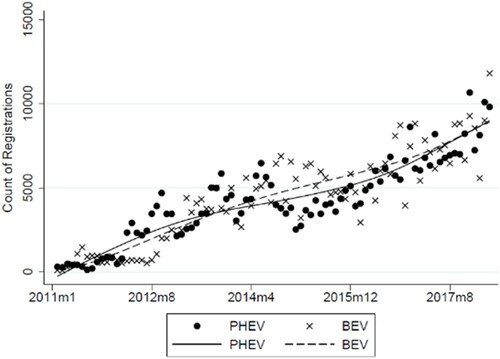
Table 1. Mean and SD for monthly BEV and PHEV sales across metro areas by region, 2011, 2015, and 2018.

Region	Vehicle type	2011	2015	2018
CA	BEV	13.6	17.7	42
		(34.1)	(49)	(173)
	PHEV	7.3	17.1	15.6
		(11.4)	(46.2)	(45.9)
West	BEV	9.7	11.9	22.4
		(26.7)	(36.8)	(111.1)
	PHEV	4.7	8.7	7.9
		(7.9)	(30.7)	(29.9)
North	BEV	1.6	4.4	9.6
		(3.9)	(11.6)	(39.8)
	PHEV	3.7	3.2	4.0
		(5.9)	(5.3)	(9.8)
South	BEV	2.8	7.5	8.4
		(4.9)	(51.8)	(28.8)
	PHEV	2.9	2.1	2.2
		(3.9)	(2.4)	(2.8)

Notes: Means and standard deviations (in parentheses) of vehicle registrations by region by year.

Our second data set consists of PM2.5 estimates for the 374 largest U.S. metropolitan areas from 2011 to 2018. The estimates are constructed from gridded daily PM2.5 levels (approximately 15 km resolution) across the 48 contiguous states (U.S. EPA 2018; Lassman et al. 2017; Burkhardt et al. 2019). We aggregate the gridded PM2.5 data by calculating the population-weighted mean for each metro area (374 counties) in our sample. We take this measure of PM2.5 pollution as a starting point, naming the variable PM2.5. However, because consumers are not likely to contemporaneously respond to air pollution with a large vehicle purchase, we adjust the measure by taking the average of air pollution over the prior four quarters to better capture cumulative impacts, and name this variable A4LPM2.5.

To construct the smoke plume data for the metro areas used in this paper, we follow the procedures detailed in Burkhardt et al. (2020).⁴ The raw data are the daily data on wildfire smoke plumes gathered by the National Oceanic and Atmospheric Administration Hazard Mapping System (HMS 2018). Wildland fires, prescribed fires, and agricultural burning generate smoke plumes that spread across the country for hundreds or thousands of miles before dissipating. This can produce elevated levels of PM2.5 (Ruminski et al. 2006; Brey et al. 2018). The Hazard Mapping System provides daily measures of smoke plumes based on satellite imagery for the entire United States (Ruminski et al. 2006; Rolph et al. 2009; HMS 2018). We associate the plume geometries with the PM2.5 grid (approximately 15 kilometres across 48 contiguous states) and assign a value of 1 if a particular grid cell was under a smoke plume for each day and 0 otherwise. We aggregate the grid cells within a metro area by calculating the population-weighted mean by day, which may result in fractions if only part of the metro area was covered by a plume. Next we sum the number of days within a quarter that a metro area was under a smoke plume. We name this variable SmokePlume.⁵ Finally, and similar to our lagged PM2.5 variable, we take the average over the prior four quarters, and name this variable A4LSmokePlume.

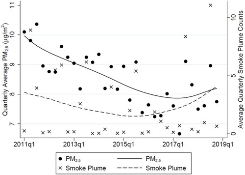
Figure 2 displays average values and trends for all U.S. metro areas in our sample for both PM2.5 and SmokePlume. PM2.5 exhibits some seasonal volatility and declines by roughly 20 percent through 2016 before recovering about a quarter of the 20 percent loss in 2017 and 2018. Unsurprisingly, SmokePlume displays extreme seasonal volatility, showing an average decline of roughly 8 percent through 2016 before increasing in 2017 and 2018. Although smoke plumes contribute to PM2.5, there is little correlation between our measures of PM2.5 and SmokePlume (see Appendix Figure 1).

Figure 2. PM2.5 and Smoke Plume, 2011–2018.

As a control variable, we include a measure (Subsidies) of the net value of state EV policy instruments, as documented for 2010–2015 in Wee, Coffman, and La Croix (2018, 2019) and extended to 2016–2018 in Hayashida, La Croix, and Coffman (2021). This variable is measured on a semi-annual basis, and changes when new policy instruments are implemented, or existing policy instruments repealed.⁶ States have specified EV policy instruments that often differ in value depending on whether a vehicle is a BEV or PHEV. Thus, we specify two different measures of Subsidies: BEV-Subsidies and PHEV-Subsidies. Each measure is the sum of the monetary value of six state-level policy instruments: five incentives (vehicle purchase incentives, home charger subsidies, reduced license and registration fees, and high occupancy vehicle lane access) and one disincentive (annual EV fees). One-time benefits are aggregated with annually accruing benefits and costs by taking the net present value over the average vehicle ownership period of six years, assuming a 5% discount rate (Wee, Coffman, and La Croix 2018). Appendix Table 1 summarizes the intervals when various state policy instruments are in effect.⁷

Lastly, our data set includes one additional variable used as a control in regressions and two more variables used to test for heterogeneous effects of A4LPM2.5 and A4LSmokePlume on EV adoptions. PublicChargers is the number of charging stations open to the public per 1,000 square miles of land by state. Two more variables, metro income per capita (Income) and metro population (Population), are used in regression specifications designed to determine whether the effects of A4LPM2.5 and A4LSmokePlume are heterogeneous with respect to metro income and metro population.

Table 2 displays descriptive statistics, definitions and sources for all variables used in the regressions reported in tables in the main text and appendix.

Table 2. Variable descriptions, summary statistics, and data sources, 2011–2018.

Variable	Description	Mean	s.d.	Min	Max	Source
EV registrations
BEV- registrations	New registrations of BEVs sold in metropolitan area a in quarter t	39	262	0	10,152	IHS Markit (2021)
PHEV- registrations	New registrations of PHEVs sold in metropolitan area a in quarter t	33	208	0	7,475	IHS Markit (2021)
Pollution
A4LPM2.5	Population-weighted PM2.5 (mg/m^3) in metropolitan area a in quarter t, measured as the average the prior four quarters	8.7	1.9	2.9	19	U.S. EPA (2018); Lassman et al. (2017); Burkhardt et al. (2018)
A4LSmoke Plume	Population-weighted smoke plume days in metropolitan area a in quarter t, measured as the average of the prior four quarters	7.3	4.8	0	27	HMS (2018)
A4LAdjusted SmokePlume	Population-weighted smoke plume days (excluding high altitude plumes) in metropolitan area a in quarter t, measured as the average of the prior four quarters	2.0	2.0	0	15	HMS (2018)
A4LAQI^a	Air Quality Index determined by the pollutant with the maximum AQI value in metropolitan area a in quarter t, measured as the average of the prior four quarters	47	12	1.7	124	U.S. EPA (2021b)
State EV Policies
BEV- Subsidies	Dollar value of vehicle purchase incentive, home charger subsidy, reduced registration fee/vehicle license tax, emissions fee abated, annual fee (negative), and HOV access value	1,479	1,837	−1,066	6,000	AFDC (2019a); govt websites; phone calls and email correspondence.
PHEV- Subsidies		1,045	1,551	−533	6,000	AFDC (2019a); govt websites; phone & email correspondences.
Other Variables
Population	Population (100,000s) in metropolitan area a in year y	9.4	22	0.5	203	U.S. Census Bureau (2010–2018a)
Income	Per capita income (100,000s) in metropolitan area a in year y (2018$)	0.3	0.1	0.1	0.6	U.S. Census Bureau (2010–2018b)
Public Chargers	Number of charging stations per 1,000 square miles (land) in state s in quarter t	554	1,179	0	10,128	AFDC (2019b); U.S. Census Bureau (2012)

Note: Each variable has 13,644 observations: 8 years × 4 quarters × 427 metro areas, including separate observations for metro areas spanning several states.

^a65 CBSAs are omitted as AQI data is not available for the entire study period.

4. Methods and theoretical foundations

We estimate all but one regression model using separate samples of quarterly data for BEVs and PHEVs over the 2011–2018 period. Our baseline specification is a model that includes a quarterly fixed effect, a metro area-by-year fixed effect, the two pollution variables (A4LPM2.5 and A4LSmokePlume) and controls for the value of state EV policy instruments (Subsidies) and the number of charging stations open to the public in the state (PublicChargers).⁸ The baseline specification is: $\begin{array}{rl}EVRe{g}_{it}=& {\text{β}}_0+{\text{β}}_{1}A4LPM{2.5}_{it}+{\text{β}}_{2}A4LSmokePlum{e}_{it}+{\text{β}}_{3}Subsidie{s}_{st}+\\ & {\text{β}}_{4}PublicCharger{s}_{st}+{\gamma }_{iy}+{\delta }_q+{ϵ}_{it}\end{array}$where $EVRe{g}_{it}$ is the count of BEV registrations in metro area i in quarter t for the BEV sample and the count of PHEV registrations for the PHEV sample, ${\gamma }_{iy}$ is the fixed effect for metro area i in year y, ${\delta }_q$ is a quarter (seasonal) fixed effect and ${ϵ}_{it}$ is an idiosyncratic error term. The quarter fixed effect absorbs unobservable shocks that are constant across metro areas but vary by season such as seasonal variation in the overall national market for BEVs and PHEVs. The metro-year fixed effect absorbs idiosyncratic shocks affecting each metro area over a given year such as metro-specific changes in vehicle sales, fuel prices, income, and population. All regressions are estimated with a Poisson pseudomaximum likelihood estimator to account for zero values on the dependent variables, overdispersion, and heteroskedasticity.⁹ Standard errors in all regressions are robust to heteroskedasticity and are clustered by metro area.

For identification, each model relies on variation within a metro area in a single year, in air pollution levels via either persistent air pollution (A4LPM2.5) or more temporary spikes in pollution (A4LSmokePlume). Although an EV that replaces a fossil-fuel-powered vehicle will displace some local pollutants, we assume that marginal EV sales are not noticeably affecting local emissions and will not affect lagged emissions. Moreover, metro area EV sales are unlikely to directly affect the probability of smoke plumes in the metro area over the eight-year interval covered by our PHEV and BEV samples.

Though we control for important factors that influence EV adoption, such as a range of subsidy programmes and the prevalence of charging stations, there may be omitted factors that could lead to endogeneity of our air pollution estimate. Specifically, short-term policies at the metro level correlated with both PM2.5 levels and EV adoption could be problematic to identification. For example, a short-term EV promotional campaign in response to seasonal pollution levels in a particular metro area could cause endogeneity on our variable of interest. For this reason, our estimates should not be interpreted as causal relationships.

Regarding a priori expectations for the signs on coefficients for the two pollution variables, the first-order effect should likely be that the relationship is positive – that consumers respond to green signals by substituting into a green good. However, in this case there are multiple vehicles from which consumers can choose. Chan and Kotchen (2014) present a generalized impure public (green) good and linear characteristics model that looks at private choice of impure public goods with both private and public characteristics. An EV is an example of an impure public good that generates private transportation services and public environmental services. In a model with just one green vehicle, say BEVs with only an electric engine, we would expect the coefficients for both pollution variables to be positive, as an increase in any type of pollution should induce substitution out of gasoline-powered vehicles into green BEVs. However, with two types of green vehicles that are substitutes, say BEVs and PHEVs with an electric engine and a gas-powered engine, coefficients for both pollution variables could be either positive or negative. In response to an increase in either A4LPM2.5 or A4LSmokePlume, we again expect a substitution out of gasoline-powered vehicles into EVs, and therefore we expect that at least one of the coefficients on A4LPM2.5 will be positive in either the BEV or the PHEV regression. Similarly, we expect that at least one of the coefficients on A4LSmokePlume will be positive in either the BEV or PHEV regressions. Chan and Kotchen (2014) show that changes in demand for green goods in their generalized model (m goods and n characteristics) ‘depend on the implicit cross-price effects among private characteristics, public characteristics, and across both’ (p. 13). In addition, when an environmental parameter changes – in this case, the level of metro pollution, there are additional income effects and complications stemming from kinked budget constraints due to the discrete choice between characteristics of BEVs and PHEVs.¹⁰

Next, we specify a series of robustness checks and estimate models that allow for heterogeneous effects of pollution in cities and states with different characteristics. First, we split the samples of EV sales into the 2011–2014 and 2015–2018 periods to check whether the estimated regression coefficients change as markets for BEVs and PHEVs changed over time. This is an important check as sales in 80 percent of metro areas increased sharply over the eight-year period and the composition of EV models in the market changed rapidly as new models entered and some models exited the market. Second, we estimate the model without California metro areas, which collectively accounted for 42 percent of EV sales over the sample period. This allows us to check whether estimates for A4LPM2.5 and A4LSmokePlume are driven by California metro areas. Third, we estimate the model using a sample that excludes metro areas with sales below the median.¹¹ This enables us to check whether metro areas in which markets for EVs have not yet emerged on a substantial scale are muting the pollution regression coefficients in the baseline regressions.

Next, we examine whether estimates of A4LPM2.5 and A4LSmokePlume are heterogeneous in metro areas with different population sizes (Population) and average per capita income (Income). We do this by estimating specifications with interaction terms between the two pollution variables and the demographic variables. Estimates could differ across metro areas with different incomes because consumers with higher incomes have more discretion in their budgets to respond voluntarily to environmental signals, and may have different preferences for different types of environmental goods. Estimates could differ across metro areas with different population sizes for a number of reasons, most of which are related to population density. Examples include greater densities of EV dealers and charging stations, availability of more EV models, smaller parking spaces, and more media/internet sources drawing attention to changes in PM2.5 and smoke plume pollution within the metro area.

We also examine whether estimates of coefficients for A4LPM2.5 and A4LSmokePlume are heterogeneous within metro areas located in states with ZEV regulations. Auto dealers and manufacturers in states with ZEV regulations are more constrained in how they adjust supply of internal combustion engine cars and EVs in response to changes in demand than auto dealers and manufacturers in states without ZEV regulations. The ZEV constraints could affect how they respond to changes in consumer demand stemming from changes in metro PM2.5 and smoke plume pollution.

We also recognize that the error terms from the PHEV and BEV regressions are likely to be correlated with each other given that the two green vehicles are substitutes (Chan and Kotchen 2014). To account for this possibility, we estimate a set of regressions on the share of BEV registrations relative to total EV (PHEV plus BEV) registrations. The ratio measure of market composition removes information in the dependent variable regarding substitution from ICEVs to EVs but can potentially provide additional insights into substitution of BEVs for PHEVs, and vice-versa, within metro areas in response to changes in the two pollution measures.

Lastly, we estimate three robustness checks. First, we rerun all regression specifications using a different measure of smoke plumes, A4LAdjustedSmokePlume, that incorporates only those smoke plumes that reach surface levels and could directly affect human exposure.¹² Second, we rerun all regression specifications using a more comprehensive measure of air pollution, Air Quality Index (AQI), that incorporates five different measures of air pollution, including PM2.5. Third, we run regression specifications for three BEV and three PHEV samples that incorporate four lags of PM2.5 and four lags of SmokePlume rather than the average of the four lags of each respective variable.

5. Empirical results

5.1. Results for regressions with BEV sample

Table 3 reports results for eight specifications of regressions with the BEV sample. In the baseline BEV specification (Table 3, column 1), the estimate for A4LPM2.5 is positive (0.19) and statistically significant at the one percent level. This means that a one unit increase in A4LPM2.5 (which indicates an increase in PM2.5 pollution) is associated with an average 21 percent increase in BEV sales within metro areas. To put this in perspective, a one-standard deviation increase in within-metro area A4LPM2.5 (1.1 units or roughly 12% of the mean across the sample) increases BEV registrations within metro areas by an average 23%. In contrast, the estimate for A4LSmokePlume is negative (−0.0077) and statistically significant at the 10 percent level. A one-standard deviation increase in within metro area A4LSmokePlume (3.26 units) decreases BEV registrations within metro areas by an average 2.5%. Thus variations in PM2.5 pollution are much more important in explaining variations in BEV sales than variations in pollution from smoke plumes.

Table 3. Poisson pseudomaximum likelihood regressions: BEV sample.

	(1)	(2)	(3)	(4)	(5)	(6)	(7)	(8)
	Full Sample	Split Sample	Split Sample	Without	With Above	Population	Income	ZEV
	2011–2018	2011–2014	2015–2018	California	Median Sales	Interaction	Interaction	Interaction
A4LPM2.5	0.190***	−0.128	0.275***	0.180***	0.196***	0.121***	0.024	0.204***
	[0.035]	[0.089]	[0.046]	[0.042]	[0.037]	[0.031]	[0.157]	[0.043]
A4LPM2.5 * Interaction Variable						0.003***	0.485	−0.050
						[0.001]	[0.486]	[0.074]
A4LSmokePlume	−0.008*	0.026***	−0.030***	−0.002	−0.009*	−0.006	0.029	−0.001
	[0.005]	[0.010]	[0.005]	[0.005]	[0.005]	[0.005]	[0.020]	[0.005]
A4LSmokePlume * Interaction Variable						−0.00007	−0.106*	−0.025***
						[0.00008]	[0.058]	[0.007]
BEV-Subsidies	0.00018	0.00009	0.00019	0.00019	0.00018	0.00017	0.00018	0.00018
	[0.00015]	[0.00007]	[0.00015]	[0.00016]	[0.00016]	[0.00015]	[0.00015]	[0.00015]
Public Chargers	0.00005	−0.00027**	0.00001	0.0013***	0.00005	0.00005	0.00005	0.00006
	[0.00004]	[0.00014]	[0.00004]	[0.0003]	[0.00004]	[0.00004]	[0.00004]	[0.00004]
Constant	4.249***	6.610***	4.065***	3.524***	4.322***	4.078***	4.197***	4.256***
	[0.402]	[0.849]	[0.533]	[0.304]	[0.422]	[0.376]	[0.439]	[0.399]
Obs	11,852	5,416	6,436	11,076	4,699	11,852	11,852	11,852
Metro-Year FE	Yes	Yes	Yes	Yes	Yes	Yes	Yes	Yes
Quarter FE	Yes	Yes	Yes	Yes	Yes	Yes	Yes	Yes

Note: Robust standard errors in brackets. All standard errors are clustered by metro area. *** p < 0.01, ** p < 0.05, * p < 0.1.

As discussed in Section 4, we estimate seven variations of our baseline regression. First, we split the sample in two at the start of 2015 and re-estimate the baseline regressions with the split samples. Results from regressions using the 2011–2014 and 2015–2018 samples are reported in columns 2 and 3, respectively. In the regression with the 2011–2014 sample (column 2), the estimated coefficient on A4LPM2.5 is negative and statistically insignificant, while the estimated coefficient on A4LSmokePlume is positive and statistically significant at the one percent level. Both results are diametrically opposite to those obtained in estimates with the full sample (column 1). However, estimated coefficients on A4LPM2.5 and A4LSmokePlume from the regression with the 2015–2018 sample (column 3) have the same signs and statistical significance as the coefficients in the baseline full-sample regressions, with the coefficients on A4LPM2.5 (0.27) and A4LSmokePlume (-0.03) both larger in absolute value than the corresponding coefficients in the baseline regressions. These larger estimates provide some indication that consumers in the U.S. vehicle market became more sensitive to environmental signals in the second half of our sample.

The next five variations – excluding California metro areas from the sample, excluding metro areas with below median sales of BEVs, including interaction variables between metro population and the two pollution measures, including interaction variables between metro income and the two pollution measures, and including interaction variables between state ZEV status and the two pollution measures – all yield estimated coefficients on A4LPM2.5 and A4LSmokePlume that follow the same pattern of signs and statistical significance as in the baseline regression. The estimated coefficient on the interaction variable between A4LPM2.5 and Population is positive and statistically significant at the five percent level (column 6), indicating a larger response to PM2.5 pollution in metro areas with higher populations. The interaction variable between Income and A4LSmokePlume is negative and statistically significant at the ten percent level, indicating a smaller response to changes in A4LSmokePlume in higher-income metro areas (column 7). Similarly, the interaction variable between ZEV and A4LPM2.5 yields a negative but statistically insignificant coefficient, while the interaction term between ZEV and A4LSmokePlume yields a negative and statistically significant coefficient, indicating the consumer response to increased smoke plumes is larger in ZEV states (column 8). Overall, the estimated coefficients on A4LPM2.5 and A4LSmokePlume are remarkably similar in five of the seven variations on the baseline regression.

All specifications include a measure of state net subsidies (BEV-Subsidies) and for the density of the state's public charger network (PublicChargers). Estimates on BEV-Subsidies are positive albeit statistically insignificant in all eight specifications. Estimated coefficients on PublicChargers are positive in seven of eight specifications albeit statistically significant in just two specifications. We note that the estimated coefficient on PublicChargers is positive and statistically significant at the one percent level in the standard specification estimated for a sample that excludes California metro areas (column 4). This result provides narrow evidence that public charger networks may be important to BEV adoption decisions in most states.

5.2. Results for regressions with PHEV sample

Table 4 reports results for eight specifications of regressions with the PHEV sample. In all eight specifications the estimated coefficients on A4LPM2.5 are negative and statistically significant at least at the five percent level. One possible explanation for this result is that increases in PM2.5 pollution induce consumers who substitute out of ICEVS to become more likely to choose a PHEV and less likely to choose a BEV. Note that the estimated coefficient in the primary specification is -0.105, which is approximately 55% of magnitude of the effect on BEV (0.19). The estimated coefficients on A4LSmokePlume tell a similarly consistent story: All are positive and seven of the eight are statistically significant at least at the five percent level. Combined with the negative estimated coefficients on A4LSmokePlume in the BEV regression, these results indicate that consumers who substitute out of ICEVS become much more likely to choose a PHEV and much less likely to choose a BEV. The interaction of A4LPM2.5 with Population suggests that this response is stronger in areas with higher population. The estimatedcoefficient on the interaction of PM2.5 and income is positive (0.005) indicating that the PHEV substitution effect is less strong in wealthier metro areas. The estimated coefficients on the interactions of A4LSmokePlume and population and A4LSmokePlume and income are not statistically significant. However, the estimated coefficient on the interaction between A4LSmokePlume and ZEV is positive and significant (0.02) indicating that consumers in metro areas with more supply regulations are more responsive to smoke-exposed days.

Table 4. Poisson pseudomaximum likelihood regressions: PHEV sample.

	(1)	(2)	(3)	(4)	(5)	(6)	(7)	(8)
	Full Sample	Split Sample	Split Sample	Without	With Above	Population	Income	ZEV
	2011–2018	2011–2014	2015–2018	California	Median Sales	Interaction	Interaction	Interaction
A4LPM2.5	−0.105***	−0.232***	−0.058**	−0.123***	−0.109***	−0.094***	−0.290***	−0.126***
	[0.030]	[0.065]	[0.024]	[0.028]	[0.032]	[0.032]	[0.085]	[0.027]
A4LPM2.5 * Interaction Variable						−0.0005*	0.548**	0.068
						[0.0003]	[0.218]	[0.044]
A4LSmokePlume	0.015***	0.030***	0.009**	0.010***	0.013***	0.014***	0.003	0.010***
	[0.004]	[0.010]	[0.004]	[0.002]	[0.004]	[0.005]	[0.016]	[0.002]
A4LSmokePlume * Interaction Variable						0.00003	0.035	0.020**
						[0.00005]	[0.046]	[0.009]
PHEV-Subsidies	−0.00002	−0.00007	−0.00001	−0.00001	−0.00002	−0.00002	−0.00002	−0.00002
	[0.00001]	[0.00010]	[0.00001]	[0.00001]	[0.00001]	[0.00001]	[0.00001]	[0.00001]
Public Chargers	−0.00006*	−0.0006***	−0.00002	−0.0002	−0.00005	−0.00006*	−0.00007**	−0.00007**
	[0.00003]	[0.00015]	[0.00002]	[0.00014]	[0.00003]	[0.00003]	[0.00003]	[0.00003]
Constant	6.776***	7.703***	6.581***	6.772***	7.012***	6.803***	6.736***	6.795***
	[0.228]	[0.598]	[0.149]	[0.190]	[0.247]	[0.233]	[0.180]	[0.178]
Obs	12,856	6,328	6,528	12,060	4,699	12,856	12,856	12,856
Metro-Year FE	Yes	Yes	Yes	Yes	Yes	Yes	Yes	Yes
Quarter FE	Yes	Yes	Yes	Yes	Yes	Yes	Yes	Yes

Note: Robust standard errors in brackets. All standard errors are clustered by metro area. *** p < 0.01, ** p < 0.05, * p < 0.1.

Similar to the BEV-focused regressions, all specifications include PHEV-Subsidies and PublicChargers. The estimated coefficients for PHEV-Subsidies are negative for all eight specifications, though not statistically significant in any specification. The estimated coefficients for PublicChargers are negative for all eight specifications, and statistically significant at least at the ten percent level in five of eight specifications. A possible explanation for the negative sign is that expansions in public charger networks are associated with additional substitution out of ICEVs into BEVs and less substitution into PHEVs. In metro areas where charging networks are becoming denser over the sample period, consumers reasonably expect that there will be fewer instances where travel options for BEV drivers are restricted due to range limits and/or range anxiety, allowing consumers to substitute out of PHEVs with their back-up gasoline-powered engines.

5.3. Results for regressions on BEV share in metro EV sales

We further explore the decision whether to choose a BEV or PHEV in Table 5, where the dependent variable is the share of BEVs in all EVs sold. Observations are dropped when the number of BEVs and the number of PHEVs sold in a county in a given quarter are both zero. The estimated coefficients on A4LPM2.5 are positive in all models and statistically significant at the one percent level in all specifications but for the one estimated with the 2011–2014 split sample which is statistically significant at the five percent level (column 2). The results support the hypothesis that increases in PM2.5 are associated with a higher likelihood that consumers who substitute out of ICEVs choose BEVs rather than PHEVs. Estimated coefficients on A4LPM2.5 interacted with metro area income and metro area population are positive and statistically significant, indicating that the air pollution effects are amplified in metro areas with higher incomes and larger populations.

Table 5. Poisson pseudomaximum likelihood estimates for share of BEVs in total EVs sold.

	(1)	(2)	(3)	(4)	(5)	(6)	(7)	(8)	(9)
	Full Sample	Split Sample	Split Sample	Without	With Above	Population	Income	ZEV	Net
	2011–2018	2011–2014	2015–2018	California	Median Sales	Interaction	Interaction	Interaction	Subsidy
A4LPM2.5	0.060***	0.056**	0.075***	0.053***	0.080***	0.051***	-0.057	0.064***	0.059***
	[0.015]	[0.023]	[0.018]	[0.016]	[0.019]	[0.015]	[0.064]	[0.018]	[0.015]
A4LPM2.5 * Interaction Variable						0.001**	0.399*	-0.003
						[0.0005]	[0.226]	[0.030]
A4LSmokePlume	0.0001	–0.004	–0.012*	0.002	–0.003	–0.0005	0.020	0.003	0.0003
	[0.005]	[0.007]	[0.006]	[0.005]	[0.005]	[0.005]	[0.024]	[0.005]	[0.005]
A4LSmokePlume * Interaction Variable						0.0001	0.070	–0.020
						[0.0001]	[0.075]	[0.013]
BEV–Subsidies	0.00000	0.00009*	0.00001	0.00001	0.00000	0.00000	0.00000	0.00000
	[0.00001]	[0.00005]	[0.00001]	[0.00001]	[0.00002]	[0.00001]	[0.00001]	[0.00001]
Net BEV–PHEV Subsidies									0.00004***
									[0.00001]
Public Chargers	0.0001***	0.00002	0.00008***	0.0008***	0.0001***	0.0001***	0.0001***	0.0001***	0.0001***
	[0.00003]	[0.0001]	[0.00003]	[0.0001]	[0.00003]	[0.00003]	[0.00003]	[0.00003]	[0.00003]
Constant	–1.329***	–1.476***	–1.349***	–1.526***	–1.464***	–1.392***	–1.363***	–1.372***	–1.341***
	[0.122]	[0.221]	[0.138]	[0.131]	[0.156]	[0.115]	[0.131]	[0.128]	[0.118]
Obs	7,894	3,090	4,804	7,298	4,699	7,894	7,894	7,894	7,894
Metro–Year FE	Yes	Yes	Yes	Yes	Yes	Yes	Yes	Yes	Yes
Quarter FE	Yes	Yes	Yes	Yes	Yes	Yes	Yes	Yes	Yes

The estimated coefficients on A4LSmokePlume vary in sign, though only the negative coefficient in the 2015–2018 sample is statistically significant at the ten percent level (Table 5, column 3). Estimated coefficients on BEV-Subsidies are close to zero and statistically insignificant but for the coefficient in the regression for the early part of the sample (2011–2014). This suggests that BEV subsidies could have played some role during the early phases of BEV adoption. We also experiment with an alternative measure of subsidies, which is the difference between BEV and PHEV subsidies, named Net BEV-PHEV-Subsidies. Results (column 9) for a specification with this subsidy variable using the full 2011–2018 sample shows an estimated coefficient (0.00004) that is positive, relatively small, and statistically significant at the one percent level.

Finally, estimated coefficients on Public Chargers in all regressions are positive and statistically significant at the one percent level in all but the 2011–2014 split-sample regression (column 2). This weakly suggests that increases in the density of the public charger network decreases range anxiety and allows more consumers to safely choose a BEV rather a PHEV. We note that the estimated coefficient is likely biased upwards, as a greater share of BEVs amongst EVs increases incentives to invest in public charger networks.

5.4. Three robustness checks

First, we estimated regression specifications with a measure of smoke plumes adjusted to include only plumes that affect surface level air quality: A4LAdjustedSmokePlume. Results are reported in Appendix Table 3 for the BEV sample and Appendix Table 4 for the PHEV sample. Estimates are broadly consistent with those obtained from regressions estimated with A4LSmokePlume, with levels of statistical significance for estimated coefficients on pollution variables lower in some specifications.

Second, we estimated regression specifications with a broad measure of metro pollution, the Air Quality Index (AQI). The U.S. EPA calculates AQI for metro areas from five air pollutants: ground-level ozone, PM2.5, carbon monoxide, sulfur dioxide, and nitrogen dioxide. Results from regression specifications replacing A4LPM2.5 with A4LAQI are reported in Appendix Table 5 for three PHEV and three BEV samples: the full sample, the sample without California metro areas, and the sample of metro areas with above median sales. Estimates are broadly consistent in signs and statistical significance of estimated coefficients with those obtained in regressions with A4LSmokePlume.

Third, we estimated regression specifications for both the PHEV and BEV samples that include four separate lags of PM2.5 and four separate lags of SmokePlume rather than averages of four lags of PM2.5 and SmokePlume. Appendix Table 5 reports results from regressions using A4LAQI instead of A4LPM2.5. Patterns of signs and statistical significance for estimated coefficients on the four lagged PM2.5 and SmokePlume variables closely correspond to the sign patterns and statistical significance for estimated coefficients on A4LPM2.5 and A4LSmokePlume. In sum, entering the four lags separately does not substantially affect estimates for PM2.5 and SmokePlume variables.

6. Discussion and conclusion

Our study shows that changes in local air pollution within U.S. metropolitan areas are associated with changes in consumer purchases of new EVs. We find a positive association between PM2.5 pollution and BEV adoption, and a negative association between PM2.5 pollution and PHEV adoption. Chan and Kotchen’s (2014) framework for analyzing choice between multiple green goods points us to the possibility of consumer substitution from PHEVs to BEVs in response to increases in PM 2.5. There was a large average decline (19 percent) in quarterly PM2.5 air pollution within the metropolitan areas in our sample. This implies that a decline in PM2.5 levels served to suppress BEV and raise PHEV adoptions.

Smoke plumes caused by wildland and agricultural fires that drift over metropolitan areas, on the other hand, are positively associated with PHEV adoption and negatively associated with BEV adoption – though this effect is relatively small in comparison to the consumer response to PM2.5. We speculate that the preference for PHEVs in response to the presence of smoke plumes may be tied to risk-averse consumers choosing the EV technology that allows more flexibility during an environmental emergency, such as an evacuation from a wildfire. Whereas our measure of PM2.5 pollution represents more persistent air pollution from local sources, our measure of smoke plumes tends to be more sporadic, seasonal, and temporary. As such, we conclude that drivers are rationally more receptive to persistent environmental signals than temporary ones, particularly given that smoke plumes always originate outside of large metropolitan areas.

Our results regarding the influence of metro pollution on EV adoption provide useful information for framing the future policy environment. If declines in metro area PM2.5 pollution continue in tandem with increases in smoke pollution, then policymakers may find that the PHEV market is expanding even in the absence of new state and federal EV policies while the BEV market is contracting. In addition, we find that increases in PM2.5 are associated with a net increase in EV adoption (BEVs increasing and PHEVs decreasing) while state-level BEV net subsidies only induce adoption in the 2011–2014 subsample of our data. This suggests that existing policy interventions may have only induced early adoption of a lesser-known technology, whereas voluntary response plays a continued role. This finding adds to the broader literature on the role of voluntary behaviour versus policy-induced behaviour (e.g. Ostrom 2000; Bayham et al. 2015; Yan et al. 2021). We emphasize that our results should not be interpreted as a justification for relaxing emissions regulations because neither state policy nor the presence of local air pollution will prompt EV adoption to the levels set by U.S. goals to curb the climate crisis. The Biden administration has set a goal of EVs accounting for 50% of new car sales by 2030.¹³ Achievement of this target clearly depends on whether consumer preferences begin to tilt towards green goods, whether technology underlying BEV and PEV models substantially improves (particularly with respect to battery weight, performance and cost), how the relative prices of EVs and conventional vehicles evolve, and the important role of supply-side interventions.

Our analysis has two important caveats. First, through the first six years of our sample (2011–2016), the level of measured smoke exposure from severity wildfire season decreased. However, over the 2017–2021 period (with the last three years beyond our sample period) the trend in wildfires changed course and the level of measured smoke exposure increased substantially. We caution that the estimated regression coefficients on SmokePlume may not be reliable indicators of future EV purchases given the large changes in SmokePlume values. Second, the markets for EVs are still relatively new with more vehicle models coming online each year, large increases in EV driving ranges, and more charging stations in every state. The changing nature of EVs offered in the market and increases in supportive infrastructure could affect the relationships between EV purchases and either measure of pollution.

Acknowledgments

We thank the participants in seminars at the University of Hawaii and University of Arizona, and in the Sixth Annual International Conference on Applied Economics in Hawaii. We also thank the University of Hawaii Economic Research Organization for financial support of this project.

Disclosure statement

No potential conflict of interest was reported by the author(s).

Additional information

Funding

This work was supported by University of Hawaii Economic Research Organization.

Notes

1 Based on the average mix of energy sources in U.S. electricity generation during 2019, the U.S. Department of Energy (DOE) estimates that a BEV typically produces the least GHG emissions, followed by a PHEV, a hybrid electric vehicle (HEV) and, lastly, a gasoline vehicle (AFDC, 2019a). Vehicle rankings by GHG emissions are somewhat different at the state level. EVs are an improvement over HEVs in most states, though in 15 coal-dependent states, HEVs still outperform EVs in terms of GHG emissions. The DOE does not provide the same level of information for local air pollutants.

2 See OECD (2020), executive summary. The OECD report focuses on BEVs and contains little information about non-exhaust PM2.5 emissions of PHEVs. Requia et al. (2018) provides a literature survey through 2017.

3 The registration data reports two separate values for vehicles sold in different parts of core-based statistical areas (CBSAs) which consist of metropolitan and micropolitan areas. Some CBSAs are located in different states and have a separate entry for the portion in each state. This expands 374 CBSAs into 427 separate CBSAs. Throughout the paper we refer to this expanded set of CBSAs as ‘metro areas’. See U.S. Census Bureau (2016) for a discussion.

4 This section follows the logic described in Burkhardt et al. (2020, 191).

5 Smoke plumes are often transported in the upper atmosphere and may not necessarily affect surface-level air quality (Rolph et al. 2009; Ford et al. 2018; Brey et al. 2018). To address the discrepancy between data from satellite imagery and what people experience on-the-ground, as a sensitivity analysis we operationalize a method described in Burkhardt et al. (2018) to probabilistically detect whether the smoke plume affected human exposure. We compare PM2.5 levels on smoke days to the three-month average PM2.5 level around a specific day. We consider a day truly smoke exposed when the PM2.5 level on that day exceeds one standard deviation of the three-month non-smoke mean. We take the estimate of smoke-exposed days in a quarter in a given county, and aggregate counties into the 427 metro areas in our sample. Next we take the average over the prior four quarters, and name this variable A4LAdjustedSmokePlume.

6 Policy data from Hayashida, La Croix, and Coffman (2021) are dated according to the enactment date of a policy. We have updated this data set to date the start of a policy as the period when it becomes effective.

7 For some state-level policy data – HOV lane access and designated parking, we gather additional data from a number of publicly-available sources. All data were collected at the state level except data on exemptions from emissions inspections. They were usually collected at the county level, but then assigned as a state-level policy based on whether the policy reached at least 50% of the population in the state. Sources include government websites, phone calls and e-mail correspondence, including the Alternative Fuels Data Center (AFDC) (2019a).

8 Increases in PublicChargers could result in consumers substituting a BEV purchase for a PHEV purchase due to the denser charging options available to drivers taking long-distance trips. However, increases or expected increases in EV registrations could also induce changes in public and private investments in the charging network open to the general public. The positive feedback from EV registrations to PublicChargers implies that the estimated coefficient on PublicChargers will be biased upwards. We also note there is very little variation in these control variables within metro areas within years.

9 We use the STATA ppmlhdfe estimator in all specifications (Correia, Guimarães, and Zylkin 2020).

10 Finally, it is possible that both coefficients on the pollution variables are negative if consumers decide to substitute away from both conventional autos and EVs into non-plug-in hybrid electric vehicles.

11 The median number of EV sales in our sample is 2 per metro area per quarter.

12 Many smoke plumes exist only in the upper atmosphere. To detect smoke plumes that are affecting surface level pollution, we adjust the HMS data to consider only smoke plumes that coincide with surface level PM2.5 measures 2 standard deviations above the background mean PM2.5 levels. In other words, our adjusted smoke plume variable is only equal to 1 when there is a smoke plume present in the atmospheric column (HMS = 1) and ambient PM2.5 is 2 standard deviations above the background mean.

13 See ‘President Biden sets a goal of 50 percent electric vehicle sales by 2030,’ New York Times, Aug. 5, 2021. https://www.nytimes.com/2021/08/05/business/biden-electric-vehicles.html (last accessed on 22 August 2021).

Appendix

Figure A1. Scatter plot of quarterly PM2.5 levels and weighted smoke plumes.

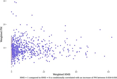
Table A1. Duration of EV policies by state, 2011–2018.

Vehicle purchase incentive (subsidy or sales tax exemption)		Home charger subsidy	Reduced vehicle license tax or registration fee		Emission inspection exemption		HOV lane exemption		Annual EV fee
BEV	PHEV		BEV	PHEV	BEV	PHEV	BEV	PHEV	BEV	PHEV
CA 11.1–18.2	CA 11.1–18.2	AZ 11.1–17.1	AZ 11.1–18.2	CT 13.1–18.2	AZ 11.1–18.2	MD 11.1–12.2	AZ 11.1–18.2	AZ 14.1–15.1	CO 14.1–18.2	CO 14.1–18.2
CO 12.1–18.2	CO 12.1–18.2	DE 15.2–18.2	CT 13.1–18.2	IL 11.1–18.2	CT 11.1–18.2	NV 11.1–18.2	CA 11.1–18.2	CA 11.1–18.2	GA 15.2–18.2	GA 15.2–18.2
CT 15.1–18.2	CT 15.1–18.2	HI 11.1–12.1	IA 11.1–14.1		MD 11.1–18.2		FL 11.1–18.2	FL 11.1–18.2	ID 15.1–18.2	ID 15.1–18.2
DE 15.2–18.2	DE 15.2–18.2	IL 13.2–15.1	IL 11.1–18.2		NC 11.1–18.2		GA 15.2–18.2	GA 15.2–18.2	IN 18.1–18.2	IN 18.1–18.2
GA 11.1–15.1	HI 11.1–12.1	LA 11.1–17.1			NH 11.1–18.2		HI 11.1–18.2	HI 11.1–18.2	MI 17.1–18.2	MI 17.1–18.2
HI 11.1–12.1	IL 11.1–15.1	MD 11.2–18.2			NM 12.1–18.2		MD 11.1–18.2	MD 11.1–18.2	MN 18.1–18.2	MO 18.1–18.2
IL 11.1–15.1	MA 14.1–18.2	MO 15.1–18.1			NV 11.1–18.2		NC 11.1–18.2	NC 11.1–18.2	MO 11.1–18.2	MS 18.2
LA 11.1–18.2	MD 11.1–18.2	NY 13.1–17.2			NY 11.1–18.2		NY 11.1–18.2	NY 11.1–18.2	MS 18.2	SC 18.1–18.2
MA 14.1–18.2	NH 18.1–18.2	OR 11.1–17.2			OR 11.1–18.2		TN 11.1–18.2	TN 11.1–18.2	NC 14.1–18.2	VA 12.2–13.1
MD 11.1–18.2	OR 11.1–11.2; 18.1–18.2				PA 11.1–18.2		UT 11.1–18.2	UT 11.1–18.2	NE 11.1–18.2	WI 18.1–18.2
NH 18.1–18.2	PA 11.1–18.2				TX 11.1–18.2		VA 11.1–18.2		SC 18.1–18.2	WV 17.2–18.2
NJ 11.1–18.2	RI 16.1–17.1								TN 17.2–18.2	WY 15.2–18.2
OK 11.1–18.2	SC 12.1–16.2								VA 12.2–18.2
OR 11.1–11.2; 18.1–18.2	TN 11.1–13.1; 15.1–16.1								WA 13.1–18.2
PA 11.1–18.2	TX 14.1–15.2; 17.2–18.2								WI 18.1–18.2
RI 16.1–17.1	UT 11.1–17.2								WV 17.2–18.2
SC 12.1–16.2	VT 14.1								WY 15.2–18.2
TN 11.1–13.1; 15.1–16.1	WA 15.2–18.1
TX 14.1–15.2; 17.2–18.2
UT 11.1–17.2
VT 14.1
WA 11.1–18.1

Table A2. State policy variable descriptions, summary statistics, and data sources: 2011–2018.

Variable	Description	Mean	S.D.	Min.	Max.	Source
EV Policies
BEV purchase incentive	Dollar value of vehicle purchase incentive (in the form of a rebate, subsidy, income tax credit, excise tax credit, or sales tax exemption) in state s in half-year t	902	1,428	0	6,000	AFDC, 2019; govt websites; phone calls and email correspondences.
PHEV purchase incentive		481	1,043	0	6,000	AFDC, 2019; govt websites; phone calls and email correspondences.
Home charger subsidy	Dollar value of home charge subsidy for hardware and/or installation in state s in half-year t	45	180	0	1,500	AFDC, 2019; govt websites; phone calls and email correspondences.
BEV reduced VLT or registration fee	Present value savings from reduced VLT or registration fee in state s over six-year vehicle ownership based on the applicable fee in the purchase period and frequency assessed	58	265	0	1,599	AFDC, 2019; govt websites; phone calls and email correspondences.
PHEV reduced VLT or registration fee		17	89	0	528	AFDC, 2019; govt websites; phone calls and email correspondences.
BEV emissions inspection fee exemption	Present value savings from emissions inspection fee exemption in state s over six-year vehicle ownership based on the applicable fee in the purchase period and frequency assessed	20	44	0	184	AFDC, 2019; govt websites; phone calls and email correspondences.
PHEV emissions inspection fee exemption		0.31	3.0	0	35	AFDC, 2019; govt websites; phone calls and email correspondences.
BEV HOV access value	Present value of HOV access value in state s over six-year vehicle ownership based on the initial purchase period value	590	1,021	0	3,493	AFDC, 2019; govt websites; phone calls and email correspondences; Texas A&M Transportation Institute, 1982–2017.
PHEV HOV access value		392	711	0	2,799	AFDC, 2019; govt websites; phone calls and email correspondences.
Annual BEV fee	Present value of the annual EV fee in state s over six-year vehicle ownership based on the initial purchase period value	95	238	0	1,139	AFDC, 2019; govt websites; phone calls and email correspondences.
Annual PHEV fee		36	151	0	1,139	AFDC, 2019; govt websites; phone calls and email correspondences.
BEV subsidies	Dollar value of vehicle purchase incentive, home charger subsidy, reduced registration fee/vehicle license tax, emissions fee abated, annual fee (−), and HOV access value weighted by population in state s at in half-year t	1,479	1,837	−1,066	6,000	AFDC, 2019; govt websites; phone calls and email correspondences.
PHEV subsidies		1,045	1,551	−533	6,000	AFDC, 2019; govt websites; phone calls and email correspondences.

Table A3. Poisson psuedomaximum likelihood regressions with A4LAdjustedSmokePlumes: BEV sample.

	(1)	(2)	(3)	(4)	(5)	(6)	(7)	(8)
	Full Sample	Split Sample	Split Sample	Without	With Above	Population	Income	ZEV
	2011–2018	2011–2014	2015–2018	California	Median Sales	Interaction	Interaction	Interaction
A4LPM2.5	0.209***	−0.119	0.293***	0.216***	0.217***	0.161***	0.084	0.243***
	[0.035]	[0.106]	[0.051]	[0.036]	[0.037]	[0.035]	[0.154]	[0.040]
A4LPM2.5 * Interaction Variable						0.002**	0.356	−0.097
						[0.001]	[0.459]	[0.073]
A4LAdjustedSmokePlume	−0.025**	0.015	−0.052**	−0.028**	−0.027**	−0.035**	−0.010	−0.030**
	[0.012]	[0.022]	[0.022]	[0.012]	[0.013]	[0.014]	[0.082]	[0.014]
A4LAdjustedSmoke Plume * Interaction Variable						0.0005**	−0.039	0.011
						[0.0003]	[0.245]	[0.029]
BEV-Subsidies	0.0002	0.0001	0.0002	0.0002	0.0002	0.0002	0.0002	0.0002
	[0.0002]	[0.0001]	[0.0002]	[0.0002]	[0.0002]	[0.0002]	[0.0002]	[0.0002]
PublicChargers	0.00004	−0.0002*	−0.00001	0.001***	0.00004	0.00004	0.00003	0.00005
	[0.00004]	[0.0001]	[0.00005]	[0.0003]	[0.00004]	[0.00004]	[0.00005]	[0.00004]
Constant	4.088***	6.610***	3.816***	3.262***	4.147***	3.973***	4.070***	4.064***
	[0.415]	[1.016]	[0.554]	[0.295]	[0.435]	[0.404]	[0.456]	[0.401]
Obs	11,852	5,416	6,436	11,076	4,699	11,852	11,852	11,852
Metro-Year FE	Yes	Yes	Yes	Yes	Yes	Yes	Yes	Yes
Quarter FE	Yes	Yes	Yes	Yes	Yes	Yes	Yes	Yes

Note: Robust standard errors in brackets. All standard errors are clustered by metro area. *** p < 0.01, ** p < 0.05, * p < 0.1.

Table A4. Poisson pseudomaximum likelihood regressions with A4LAdjustedSmokePlumes: PHEV sample.

	(1)	(2)	(3)	(4)	(5)	(6)	(7)	(8)
	Full Sample	Split Sample	Split Sample	Without	With Above	Population	Income	ZEV
	2011–2018	2011–2014	2015–2018	California	Median Sales	Interaction	Interaction	Interaction
A4LPM2.5	−0.098***	−0.252***	−0.068***	−0.120***	−0.096***	−0.081***	−0.275***	−0.117***
	[0.022]	[0.051]	[0.022]	[0.014]	[0.024]	[0.022]	[0.068]	[0.014]
A4LPM2.5 * Interaction Variable						−0.0007***	0.522**	0.063
						[0.0002]	[0.208]	[0.042]
A4LAdjustedSmokePlume	0.010	0.015	0.019***	0.009	0.004	0.005	−0.037	0.004
	[0.013]	[0.036]	[0.005]	[0.015]	[0.013]	[0.014]	[0.048]	[0.016]
A4LAdjustedSmokePlume * Interaction Variable						0.0002**	0.145	0.027
						[0.0001]	[0.115]	[0.018]
PHEV-Subsidies	−0.00002	−0.00007	−0.00001	−0.00002	−0.00002	−0.00002	−0.00002	−0.00002
	[0.00001]	[0.00009]	[0.00001]	[0.00001]	[0.00001]	[0.00001]	[0.00001]	[0.00001]
PublicChargers	−0.00006**	−0.0005***	−0.00001	−0.0002*	−0.00005*	−0.00006**	−0.00006**	−0.00006**
	[0.00003]	[0.0002]	[0.00002]	[0.0001]	[0.00003]	[0.00003]	[0.00003]	[0.00003]
Constant	6.795***	8.051***	6.680***	6.808***	6.985***	6.834***	6.752***	6.802***
	[0.174]	[0.466]	[0.151]	[0.110]	[0.188]	[0.182]	[0.133]	[0.137]
Obs	12,856	6,328	6,528	12,060	4,699	12,856	12,856	12,856
Metro-Year FE	Yes	Yes	Yes	Yes	Yes	Yes	Yes	Yes
Quarter FE	Yes	Yes	Yes	Yes	Yes	Yes	Yes	Yes

Note: Robust standard errors in brackets. All standard errors are clustered by metro area. *** p < 0.01, ** p < 0.05, * p < 0.1.

Table A5. Poisson pseudomaximum likelihood regressions with AQI pollution: PHEV and BEV samples.

	PHEV	PHEV	PHEV	BEV	BEV	BEV
	(1)	(2)	(3)	(4)	(5)	(6)
	Full Sample	Without	With Above	Full Sample	Without	With Above
	2011–2018	California	Median Sales	2011–2018	California	Median Sales
A4LAQI	−0.024***	−0.023**	−0.026***	0.032***	0.024**	0.032***
	[0.008]	[0.011]	[0.009]	[0.011]	[0.011]	[0.011]
A4LSmokePlume	0.016***	0.011***	0.015***	−0.008*	0.0005	−0.009**
	[0.004]	[0.003]	[0.004]	[0.004]	[0.004]	[0.004]
Subsidy	−0.00001	−0.00001	−0.00001	0.0002	0.0002	0.0002
	[0.00001]	[0.00001]	[0.00001]	[0.0002]	[0.0002]	[0.0002]
Public Chargers	−0.00007**	−0.0002	−0.00006**	0.00008*	0.001***	0.00008*
	[0.00003]	[0.0002]	[0.00003]	[0.00004]	[0.000]	[0.00004]
Constant	7.222***	6.991***	7.499***	4.130***	3.845***	4.226***
	[0.404]	[0.472]	[0.418]	[0.364]	[0.423]	[0.371]
Obs	11,436	10,640	4,424	10,632	9,856	4,424
Metro-Year FE	Yes	Yes	Yes	Yes	Yes	Yes
Quarter FE	Yes	Yes	Yes	Yes	Yes	Yes

Note: Robust standard errors in brackets. All standard errors are clustered by metro area. *** p < 0.01, ** p < 0.05, * p < 0.1.

Table A6. Poisson pseudomaximum likelihood regressions with lagged PM2.5 and smoke plume variables: PHEV and BEV samples.

	PHEV	PHEV	PHEV	BEV	BEV	BEV
	(1)	(2)	(3)	(4)	(5)	(6)
	Full Sample	Without	With Above	Full Sample	Without	With Above
	2011–2018	California	Median Sales	2011–2018	California	Median Sales
Subsidy	−0.00002	−0.00001	−0.00002	0.00018	0.0002	0.0002
	[0.00001]	[0.00001]	[0.00001]	[0.00014]	[0.0001]	[0.0001]
PM2.5-L1	−0.016	−0.019	−0.019*	0.0382***	0.032***	0.038***
	[0.010]	[0.012]	[0.011]	[0.009]	[0.009]	[0.010]
PM2.5-L2	−0.026**	−0.037***	−0.028**	0.036***	0.020	0.037***
	[0.010]	[0.012]	[0.012]	[0.011]	[0.015]	[0.012]
PM2.5-L3	−0.020**	−0.031***	−0.023**	0.040***	0.027*	0.041***
	[0.009]	[0.011]	[0.010]	[0.011]	[0.014]	[0.012]
PM2.5-L4	−0.030***	−0.031***	−0.033***	0.042***	0.020	0.044***
	[0.005]	[0.005]	[0.006]	[0.013]	[0.018]	[0.014]
SmokePlume-L1	0.004***	0.002**	0.004***	−0.00009	0.005***	−0.0004
	[0.001]	[0.001]	[0.001]	[0.00194]	[0.002]	[0.002]
SmokePlume-L2	0.006***	0.004***	0.005***	−0.006***	−0.009***	−0.007***
	[0.002]	[0.001]	[0.002]	[0.002]	[0.002]	[0.002]
SmokePlume-L3	0.002*	0.0006	0.001	−0.004***	−0.005**	−0.004***
	[0.001]	[0.0009]	[0.001]	[0.001]	[0.002]	[0.002]
SmokePlume-L4	0.003***	0.003**	0.003**	−0.001	−0.0002	−0.001
	[0.001]	[0.001]	[0.001]	[0.001]	[0.002]	[0.001]
Public Chargers	−0.00002	−0.0002	−0.00002	0.00000	0.002***	0.00000
	[0.00003]	[0.0002]	[0.00002]	[0.00005]	[0.0002]	[0.00005]
Constant	6.610***	6.719***	6.909***	4.639***	4.135***	4.751***
	[0.276]	[0.245]	[0.315]	[0.359]	[0.344]	[0.377]
Obs	12,856	12,060	4,699	11,852	11,076	4,699
Metro-Year FE	Yes	Yes	Yes	Yes	Yes	Yes
Quarter FE	Yes	Yes	Yes	Yes	Yes	Yes

Note: Robust standard errors in brackets. All standard errors are clustered by metro area. *** p < 0.01, ** p < 0.05, * p < 0.1.

References

- AFDC (Alternative Fuels Data Center). 2019a. State Laws and Incentives. U.S. Department of Energy. https://afdc.energy.gov/laws/state (last accessed on 5 October 2019).
- AFDC (Alternative Fuels Data Center). 2019b. Electric Vehicle Charging Station Locator. U.S. Department of Energy. https://afdc.energy.gov/fuels/electricity_locations.html (last accessed on 5 October 2019).
- Ambrose, H., A. Kendall, M. Lozano, S. Wachche, and L. Fulton. 2020. “Trends in Life Cycle Greenhouse Gas Emissions of Future Light Duty Electric Vehicles.” Transportation Research Part D: Transport and Environment 81: 102287. doi:10.1016/j.trd.2020.102287.
- Bayham, J., N. V. Kuminoff, Q. Gunn, and E. P. Fenichel. 2015. “Measured Voluntary Avoidance Behaviour During the 2009 A/H1N1 Epidemic.” Proceedings of the Royal Society B: Biological Sciences 282: 20150814. doi:10.1098/rspb.2015.0814.
- Bento, D., D. Kaffine, K. Roth, and M. Zaragoza-Watkins. 2014. “The Effects of Regulation in the Presence of Multiple Unpriced Externalities: Evidence from the Transportation Sector.” American Economic Journal: Economic Policy 6 (3): 1–29. doi:10.1257/pol.6.3.1.
- Berhane, K., C. Chang, and R. McConnell. 2016. “Association of Changes in Air Quality with Bronchitic Symptoms in Children in California, 1993–2012.” Journal of the American Medical Association 315 (14): 1491–1501. doi:10.1001/jama.2016.3444.
- Brady, J., and M. O’Mahony. 2011. “Travel to Work in Dublin. The Potential Impacts of Electric Vehicles on Climate Change and Urban Air Quality.” Transportation Research Part D 16 (2): 188–193. doi:10.1016/j.trd.2010.09.006.
- Brey, S., M. Ruminski, S. Atwood, and E. Fischer. 2018. “Connecting Smoke Plumes to Sources Using Hazard Mapping System (hms) Smoke and Fire Location Data Over North America.” Atmospheric Chemistry and Physics 18 (1): 1745–1761. doi:10.5194/acp-18-1745-2018.
- Burke, M., A. Driscoll, S. Heft-Neal, J. Xue, J. Burney, and M. Wara. 2021. “The Changing Risk and Burden of Wildfire in the United States.” Proceedings of the National Academy of Sciences 118 (2): e2011048118. doi:10.1073/pnas.2011048118.
- Burkhardt J., J. Bayham, A. Wilson, E. Carter, J. D. Berman, K. O’Dell, B. Ford, E. V. Fischer, and J. R. Pierce. 2019. “The Effect of Pollution on Aggressive Behavior: Evidence from Wildfire Smoke and Crime.” Working Paper.
- Burkhardt, J., J. Bayham, A. Wilson, J. D. Berman, K. O’Dell, B. Ford, E. V. Fischer, and J. R. Pierce. 2020. “The Relationship Between Monthly Air Pollution and Violent Crime across the United States.” Journal of Environmental Economics and Policy 9 (2): 188–205. doi:10.1080/21606544.2019.1630014.
- Carley, S., R. Krause, B. Lane, and J. Graham. 2013. “Intent to Purchase a Plug-In Electric Vehicle: A Survey of Early Impressions in Large U.S. Cities.” Transportation Research Part D 18: 39–45. doi:10.1016/j.trd.2012.09.007.
- Carley, S., S. Siddiki, and S. Nicholson-Crotty. 2019. “Evolution of Plug-In Electric Vehicle Demand: Assessing Consumer Perceptions and Intent to Purchase Over Time.” Transportation Resarch Part D 70: 94–111. doi:10.1016/j.trd.2019.04.002.
- Chan, N. W., and M. J. Kotchen. 2014. “A Generalized Impure Public Good and Linear Characteristics Model of Green Consumption.” Resource and Energy Economics 37: 1–16. doi:10.1016/j.reseneeco.2014.04.001.
- Coffman, M., P. Bernstein, and S. Wee. 2017. “Electric Vehicles Revisited: A Review of Factors that Affect Adoption.” Transport Reviews 37 (1): 79–93. doi:10.1080/01441647.2016.1217282.
- Correia, S., P. Guimarães, and T. Zylkin. 2020. “Fast Poisson Estimation with High-Dimensional Fixed Effects.” Stata Journal 20: 95–115. doi:10.1177/1536867X20909691.
- Ferrero, E., S. Alessandrini, and A. Balanzino. 2016. “Impact of the Electric Vehicles on the Air Pollution from a Highway.” Applied Energy 169: 450–459. doi:10.1016/j.apenergy.2016.01.098.
- Fevang, E., E. Figenbaum, L. Fridstrøm, A. H. Halse, K. E. Hauge, B. G. Johansen, and O. Raaum. 2021. “Who Goes Electric? The Anatomy of Electric Car Ownership in Norway.” Transportation Research Part D: Transport and Environment 92: 102727. doi:10.1016/j.trd.2021.102727.
- Ford, B., M. Val Martin, S. Zelasky, E. Fischer, S. Anenberg, C. Heald, and J. Pierce. 2018. “Future Fire Impacts on Smoke Concentrations, Visibility, and Health in the Contiguous United States.” GeoHealth 2 (8): 229–247. doi:10.1029/2018GH000144.
- Guo, J., X. Zhang, F. Gu, H. Zhang, and Y. Fan. 2020. “Does Air Pollution Stimulate Electric Vehicle Sales? Empirical Evidence from Twenty Major Cities in China.” Journal of Cleaner Production 249: 119372. doi:10.1016/j.jclepro.2019.119372.
- Hackbarth, A., and R. Madlener. 2013. “Consumer Preferences for Alternative Fuel Vehicles: A Discrete Choice Analysis.” Transportation Research Part D 25: 5–17. doi:10.1016/j.trd.2013.07.002.
- Halliday, T. J., J. Lynham, and A. de Paula. 2018. “Vog: Using Volcanic Eruptions to Estimate the Health Costs of Particulates.” Economic Journal 129 (620): 1782–1816. doi:10.1111/ecoj.12609.
- Haustein, S., and A. Jensen. 2018. “Factors of Electric Vehicle Adoption: A Comparison of Conventional and Electric Car Users Based on an Exended Theory of Planned Behavior.” International Journal of Sustainable Transportation 12 (7): 484–496. doi:10.1080/15568318.2017.1398790.
- Hayashida, S., S. La Croix, and M. Coffman. 2021. “Understanding Changes in Electric Vehicle Policies in the U.S. States, 2010–2018.” Transport Policy 103: 211–223. doi:10.1016/j.tranpol.2021.01.001.
- Hidrue, M., G. Parsons, W. Kempton, and M. Gardner. 2011. “Willingness to Pay for Electric Vehicles and their Attributes.” Resource and Energy Economics 3: 686–705. doi:10.1016/j.reseneeco.2011.02.002.
- Holland, S., E. Mansur, N. Muller, and A. Yates. 2016. “Are There Environmental Benefits from Driving Electric Vehicles? The Importance of Local Factors.” American Economic Review 106: 3700–3729. doi:10.1257/aer.20150897.
- Holland, S., E. Mansur, N. Muller, and A. Yates. 2020. “Decompositions and Policy Consequences of an Extraordinary Decline in Air Pollution from Electricity Generation.” American Economic Journal: Economic Policy 12 (4): 244–274. doi:10.1257/pol.20190390.
- HMS. 2018. “Smoke Plume Shape Files 2006–2013.” https://www.ospo.noaa.gov/Products/land/hms.html (last accessed 11 June 2019).
- IHS Markit. 2020. Dataset of New Vehicle Registration by Metro Area, 2011–2018.
- IHS Markit. 2021. Dataset of Electric Vehicle Retail New Registrations by CBSA/Metropolitan Area, Cars and Light Trucks, 2011-2018.
- Jenn, A., K. Springel, and A. R. Gopal. 2018. “Effectiveness of Electric Vehicle Incentives in the United States.” Energy Policy 119: 349–356. doi:10.1016/j.enpol.2018.04.065.
- Jenn, A., J. Lee, S. Hardman, and G. Tal. 2020. “An in-Depth Examination of Electric Vehicle Incentives: Consumer Heterogeneity and Changing Response Over Time.” Transportation Research Part A 132: 97–109. doi:10.1016/j.tra.2019.11.004.
- Larsen, A. E., B. J. Reich, M. Ruminski, and A. G. Rappold. 2018. “Impacts of Fire Smoke Plumes on Regional Air Quality, 2006–2013.” Journal of Exposure Science & Environmental Epidemiology 28 (4): 319–327. doi:10.1038/s41370-017-0013-x.
- Lassman, W., B. Ford, R. W. Gan, G. Pfister, S. Magzamen, E. V. Fischer, and J. R. Pierce. 2017. “Spatial and Temporal Estimates of Population Exposure to Wildfire Smoke During the Washington State 2012 Wildfire Season Using Blended Model, Satellite, and in Situ Data.” GeoHealth 1 (3): 106–121. doi:10.1002/2017GH000049.
- Lei, R., S. Feng, and T. Lauvaux. 2021. “Country-Scale Trends in Air Pollution and Fossil Fuel CO2 Emissions During 2001–2018: Confronting the Roles of National Policies and Economic Growth.” Environmental Research Letters 16: 014006. doi:10.1088/1748-9326/abc9e1.
- Muehlegger, E., and D. Rapson. 2020. “Correcting Estimates of Electric Vehicle Emissions Abatement: Implications for Climate Policy.” NBER Working Paper No. 27197. https://www.nber.org/system/files/working_papers/w27197/w27197.pdf.
- O’Dell, K., K. Bilsback, B. Ford, S. E. Martenies, S. Magzamen, E. V. Fischer, and J. R. Pierce. 2021. “Estimated Mortality and Morbidity Attributable to Smoke Plumes in the United States: Not Just a Western US Problem.” GeoHealth 5: e2021GH000457. doi:10.1029/2021GH000457.
- Okada, T., T. Tamaki, and S. Managi. 2019. “Effect of Environmental Awareness on Purchase Intention and Satisfaction Pertaining to Electric Vehicles in Japan.” Transportation Research Part D, Transport and Environment 67: 503–513. doi:10.1016/j.trd.2019.01.012.
- Organisation for Economic Co-operation and Development (OECD). 2020. “Non-exhaust Particulate Emissions from Road Transport: An Ignored Environmental Policy Challenge.” Paris : OECD Publishing. doi:10.1787/4a4dc6ca-en
- Ostrom, E. 2000. “Crowding Out Citizenship.” Scandinavian Political Studies 23: 3–16. doi:10.1111/1467-9477.00028.
- Requia, W. J., M. Mohamed, C. D. Higgins, A. Arain, and M. Ferguson. 2018. “How Clean Are Electric Vehicles? Evidence-Based Review of the Effects of Electric Mobility on Air Pollutants, Greenhouse Gas Emissions and Human Health.” Atmospheric Environment 185: 64–77. doi:10.1016/j.atmosenv.2018.04.040.
- Rolph, G. D., R. R. Draxler, A. F. Stein, A. Taylor, M. G. Ruminski, S. Kondragunta, J. Zeng, et al. 2009. “Description and Verification of the NOAA Smoke Forecasting System: The 2007 Fire Season.” Weather and Forecasting 24 (2): 361–378. doi:10.1175/2008WAF2222165.1.
- Ruminski, M., S. Kondragunta, R. Draxler, and J. Zeng. 2006. “Recent Changes to the Hazard Mapping System.” In 15th International Emission Inventory Conference. New Orleans, Louisiana, May 15–18, 2006.
- Shi, H., S. Wang, and D. Zhao. 2017. “Exploring Urban Resident’s Vehicular PM2.5 Reduction Behavior Intention: An Application of the Extended Theory of Planned Behavior.” Journal of Cleaner Production 147: 603–613. doi:10.1016/j.jclepro.2017.01.108.
- Shewmake, S., and L. Jarvis. 2014. “Hybrid Cars and HOV Lanes.” Transportation Research Part A 67: 304–319. doi:10.1016/j.tra.2014.07.004.
- Schöllnhammer, T., H. Hebbinghaus, S. Wurzler, and T. Schultz. 2014. “Effects of Electric Vehicles on Air Quality in Street Canyons.” Meteorologische Zeitschrift 23 (3): 331–336. doi:10.1127/metz/2014/0540.
- Sexton, S. E., and A. L. Sexton. 2014. “Conspicuous Conservation: The Prius Halo and Willingness to Pay for Environmental Bona Fides.” Journal of Environmental Economics and Management 67: 303–317. doi:10.1016/j.jeem.2013.11.004.
- Soret, A., M. Guevara, and J. M. Baldasano. 2014. “The Potential Impacts of Electric Vehicles on Air Quality in the Urban Areas of Barcelona and Madrid (Spain).” Atmospheric Environment 99: 51–63. doi:10.1016/j.atmosenv.2014.09.048.
- Soriano, J. B., P. J. Kendrick, K. R. Paulso, V. Gupta, T. Vos., and Global Burden of Disease (GBD) Chronic Respiratory Disease Collaborators. 2020. “Prevalence and Attributable Health Burden of Chronic Respiratory Diseases, 1990–2017: A Systematic Analysis for the Global Burden of Disease Study 2017.” Lancet Respiratory Medicine 8: 585–596. doi:10.1016/s2213-2600(20)30105-3.
- Timmers, V. R. J. H., and P. A. J. Achten. 2016. “Non-exhaust PM Emissions from Electric Vehicles.” Atmospheric Environment 134: 10–17. doi:10.1016/j.atmosenv.2016.03.017.
- U.S. Census Bureau. 2010–2018a. Table B01003. Total State Population. 1-Year Estimates.
- U.S. Census Bureau 2010–2018b. Annual Estimates of the Resident Population for Metropolitan Statistical Areas in the United States and Puerto Rico: April 1, 2010 to July 1, 2019.
- U.S. Census Bureau. 2012. State Area Measurements and Internal Point Coordinates. https://www.census.gov/geo/reference/state-area.html (last accessed 26 July 2017).
- U.S. Census Bureau. 2016. Core-Based Statistical Areas. https://www.census.gov/topics/housing/housing-patterns/about/core-based-statistical-areas.html (last accessed on 20 August 2021).
- U.S. Environmental Protection Agency (EPAa). 2018. Air Quality System Data Mart. http://www.epa.gov/ttn/airs/aqsdatamart (last accessed on 21 August 2021).
- U.S. Environmental Protection Agency. 2021b. Pre-Generated Data Files. https://aqs.epa.gov/aqsweb/airdata/download_files.html (last accessed 29 August 2021).
- U.S. Environmental Protection Agency (EPA). 2021a. Green Vehicle Guide, Light Duty Vehicle Emissions. https://www.epa.gov/greenvehicles/light-duty-vehicle-emissions (last accessed on 21 August 2021).
- Wee, S., M. Coffman, and S. La Croix. 2018. “Do Electric Vehicle Incentives Matter? Evidence from the 50 U.S. States.” Research Policy 47 (9): 1601–1610. doi:10.1016/j.respol.2018.05.003.
- Wee, S., M. Coffman, and S. La Croix. 2019. “Data on U.S. State-Level Electric Vehicle Policies, 2010–2015.” Data in Brief 23. doi:10.1016/j.dib.2019.01.006.
- White, L. V., and N. D. Sintov. 2017. “You Are What You Drive: Environmentalist and Social Innovator Symbolism Drives Electric Vehicle Adoption Intentions.” Transportation Research Part A 99: 94–113. doi:10.1016/j.tra.2017.03.008.
- Xing, J., B. Leard, and S. Li. 2021. “What Does an Electric Vehicle Replace?” NBER Working Paper 25771. https://www.nber.org/system/files/working_papers/w25771/w25771.pdf.
- Yan, Y., A. A. Malik, J. Bayham, E. P. Fenichel, C. Couzens, and S. B. Omer. 2021. “Measuring Voluntary and Policy-Induced Social Distancing Behavior During the COVID-19 Pandemic.” Proceedings of the National Academy of Sciences 118 (16): e2008814118. doi:10.1073/pnas.2008814118.
- Zhang, Y., Y. Yu, and B. Zhou. 2011. “Analyzing Public Awareness and Acceptance of Alternative Fuel Vehicles in China: The Case of EV.” Energy Policy 39: 7015–7024. doi:10.1016/j.enpol.2011.07.055.