Abstract
Consider an input material with a nonconforming probability that is used for the production of a product through a deteriorating process, which is initially maintained in an in-control state, but can randomly shift into an out-of-control state after some products are produced. To economically control the total quality-related cost for a given production lot, an optimal inspection policy for the products and their input materials is proposed. Furthermore, under the optimal inspection policy, a decision on the optimal production lot size is also incorporated. The unique properties and conditions that give the optimal production lot size are explored. Numerical examples are given to illustrate our proposed inspection and production model. The effects of the model's parameter values, such as inspection error rate, unit inspection cost for the input material, unit inspection cost for the product, etc., on the optimal solution are investigated. Finally, some useful insights that should help industrial operations are presented.
Introduction
Not only product quality, but also cost, is usually a major consideration when developing an order winning strategy for a company. However, high product quality always leads to a higher cost, and vice versa. Thus, the trade-off between the two above-mentioned business competitive factors is an important issue. When the products are produced by a deteriorating production system with a geometric shift distribution, in order to balance the set-up cost of production, the inventory holding cost and the product quality cost, Porteus (Citation1986) uses a small lot size that is always smaller than the traditional economic production lot size. This reduces the number of nonconforming products, where the nonconforming products are produced once the process shifts into an out-of-control state. Later, Wang and Sheu (Citation2003) extend Porteus's (Citation1986) model to allow for the process to have a general discrete shift distribution and some of the properties that relate to optimal production lot size were explored by them.
Regardless of the decision on the optimal production lot size, Raz, Herer, and Grosfeld-Nir (Citation2000) develop an economic offline inspection and disposition policy for a given production lot size, where the process is assumed to have a geometric shift distribution. Two recursive equations are used by them to solve the problem of inspection and disposition. Sheu, Chen, Wang, and Shin (Citation2003) further expanded on this in order to deal with the situation where two types of inspection errors exist in the Raz et al.'s (2000) model. However, in Sheu et al.'s (2003) model, they use process life with the property of memorylessness to develop their proposed model. However, the property of memorylessness does not hold when inspection errors are considered. In such cases, referring to Raz et al.'s (2000) concept, an extra index needs to be used to record the starting position of the discussed sub-batch when making the decision-related to inspection and disposition, and a modified model was proposed by Wang (Citation2007). This model is different from that of Sheu et al. (Citation2003) who investigated the effect of inspection errors on inspection and disposition policy. Tzimerman and Herer (Citation2009) used product inspection results to infer the shift point in the production lot using a predetermined confidence level when inspection errors exist; specifically they used an entropy function to select which product should be inspected, the aim being to maximally decrease the entropy.
Lot sizing and product inspection, two separated product quality control mechanisms, have been integrated in previous studies. For example, the product inspection policy proposed by Djamaludin, Murthy, and Wilson (Citation1994), where the products produced toward the end of the production lot should be inspected, is used by Wang and Sheu(Citation2001). Similarly, Hu and Zong (Citation2009) used these factors to integrate the policy of production planning and product inspection/reworking.
Nevertheless, product quality not only depends on the quality of the process but also on the quality of the input materials. Tagaras and Lee (Citation1996) studied the effect of the nonconforming probability of the input materials on material inspection policy and vendor selection when the purchase cost depends on the proportion of the nonconforming materials. Motivated by Tagaras Lee's (1996) concept, Wang, Dohi, and Tsai (Citation2010) propose a production and material inspection model where the input materials inspection policy and production lot size are determined simultaneously. However, the role of the product inspection policy in possibly reducing the quality-related cost is ignored. Therefore, in this paper, we integrate the inspection policy of the products and their input materials with the production lot size in a system where two types of inspection errors are considered.
The rest of this paper is organized as follows. Section 2 describes the proposed inspection and production model. The properties for the optimal inspection policy and of the production lot size are explored in Section 3. Numerical examples are given in Section 4 to illustrate our proposed model. Finally, some conclusions are made in Section 5.
2. The model of inspection and production
In this paper, it is assumed that an input material is used to produce a product through a deteriorating production system, where the process is maintained in an in-control state at the beginning of each production lot with a cost A>0, and that it may randomly shift from an in-control state to an out-of-control state during production; furthermore, let be the probability that the first j products are produced in an in-control state and
be the probability that the process has shifted into an out-of-control state before or when the jth product is produced. Note that once the process shifts into an out-of-control state, it remains there until the end of the production lot. In addition, the input material is classified as nonconforming and conforming with probability p and 1−p, respectively. A product is conforming only when its input material is conforming and is produced in an in-control state; otherwise, a nonconforming product will be produced. Here, let B be the variable cost for producing a product including the cost of the input material, R′ be the unit revenue of selling a conforming product and c′d be the unit cost of selling a nonconforming product (i.e. unit warranty cost), where R′>B>0.
To control the quality of the input materials and products, an unreliable inspection is considered to be performed with unit inspection cost and
for an input material and a product, respectively; more precisely, let α0 (α1) be the type I inspection error for an input material (a product), i.e. the probability of classifying a conforming input material (product) into a nonconforming material (product), and β0 (β1) be the type II inspection error for an input material (product), i.e. the probability of classifying a nonconforming material (product) into a conforming material (product). Once an input material (or a product) has been inspected to be nonconforming, it will be replaced by a conforming material with unit cost
(or to be sold as a substandard product with a unit revenue s, where R′>s≥0).
3. Optimal inspection and production policy
Given a production lot with a size of n, under an inspection policy (Ij, Kj) for j=1, 2, … , n, the expected total revenue is given by
In the following text, we first fix the production lot size n and explore the optimal inspection policy for j=1, 2, … , n, which maximizes Equation (1). Then, the decision on the optimal production lot size (n*) is incorporated.
3.1 Inspection process
The following indicator variables are denoted to express the status as to whether the jth product and its input materials have been inspected or not. Let Ij=0 (or 1) represent the input material used to produce the jth product has not been inspected (or has been inspected) for j=1, 2, … , n, and Kj=0 (or 1) represent the jth product has not been inspected (or has been inspected) before selling to the market, for j=1, 2, … , n.
Consider an input material is used to produce the jth product. When the input material is considered to be inspected, the resulting probability that the inspected material will be classified as conforming given that the input material is conforming or nonconforming, which are given by and
, respectively (also see Avinadav & Raz, Citation2003). This implies that the input material will be classified as nonconforming with probability
, or equivalent to
The jth product will be sold when it is inspected to be conforming; however, its real quality may be conforming or nonconforming. Alternatively, it will be sold as a substandard product without incurring any warrant cost once it is inspected to be nonconforming. The related probabilities are obtained as follows.
The jth product will be sold when its real quality status is conforming if (i) it uses a conforming material for production (with probability ) in an in-control state (with probability
) and (ii) it is inspected to be conforming (i.e. not to commit the type I inspection error or un-inspected with probability
). Thus, the resulting probability is given by
3.2 Optimal inspection policy
The optimal inspection policy for the jth product and its input material, , can be obtained by comparing the following revenues that result from the four inspection policies, (0,0), (1,0), (0,1) and (1,1):
,
, ERj (Ij
and
, where
,
,
,
,
,
,
and
.
Firstly, we investigate the case that the optimal inspection policy for the jth product is . That is, we explore the conditions that
dominates (1,0), (0,1) and (1,1).
If is superior to
, then from Equation (8) one needs the following condition to be hold:
Since
decreases as j increases, one can conclude the following decision rule, namely decision rule 1 (DR 1): let
Next, the inspection policy is superior to
if and only if
. Using a similar approach to obtain DR 1, one can conclude decision rule 2; (DR 2): let
Again, the requirement that inspection policy is superior to
is given by
Case 1 If
, then Equation (12) is equivalently to
This indicates that when the last inequality holds, the inspection policy
dominates
. Utilizing the property that
is decreasing when j is increasing, one has the following decision rule (DR 3-1): let
Case 2 If
, then a similar approach to Case 1 can be used to obtain the decision rule (DR 3-2): let
Case 3 If
, then it is easy to obtain the optimal inspection policy for the jth product and its input material, namely decision rule 3-3; (DR 3-3): if
, then
always dominates
, and one can set j32=∞ if DR 3-2 is adopted (alternatively, one can set j31=0 if one wish to adopt DR 3-1); otherwise,
is superior to
, and one can set j32=0 when DR 2 is adopted (alternatively, one can adopt DR 3-1 by setting j31=∞).
Next, we investigated the case that . That is, we would like to know that when does
dominate (1,0) and (0,1). Note that the comparisons between (1,1) and (0,0) are given in DR 3.
For the jth product, the condition that the inspection policy is superior to
is
Using a similar approach to DR 4, one can conclude the following decision rule (DR 5) when comparing two inspection policies, (Ij, Kj)=(0,1) and (1,1): let
Finally, the comparisons between and
can be analyzed as follows. It is easy to see that
is superior to
if and only if
Using the similar analysis to that used to obtain DR 1, the comparisons between
and
can be concluded by the following decision rule (DR 6): let
Based on DRs 1–6, the following proposition is proposed to determine the optimal inspection policy for a given production lot with a size of n≥1. The proofs are given in Appendix 1.
Proposition 1
Let and
where
.
(a) If p>λ, we have
] If p<λ, we have
] If p=λ, if
then we have
Propositions 1 shows that the input materials used for the products produced at the initial segment of the production lot should be inspected; on the other hand, the products produced at the tailed segment of the production lot should also be inspected. The inspection policy that both the products and their input materials should be inspected or should not be inspected occurs for the products produced in middle part of the production lot. Note that when the input quality is perfect, i.e. p=0, one has j1=1 from DR 1, and hence the inspection policy of is never optimal. On the other hand, when the unit product inspection cost is high, i.e.
, one has j2=∞ from DR 2. In this case, one can see that the inspection policy
is never optimal.
Remark 1 The lot-sizing model proposed by Porteus (Citation1986) is adequate if the optimal inspection policy is for j=1, 2, … , n. One situation for such a case is when (see Proposition 1(b)) a perfect input material is used (i.e. p=0) and the expected resulting cost of both the product and its input material are inspected is less than the maximal cost savings for a nonconforming product that has been inspected, i.e. the inequality
holds, which implies that j32=∞ (see DR 3-2).
3.3 Optimal production lot size
From Proposition 1(a), when p>λ, under the optimal inspection policy, the expected total revenue for a production lot size n≥1 is given by
The following proposition proposed the properties of the optimal production lot size n* that maximizes the total revenue given in Equation (20), and the proofs are given in Appendix 3.
Proposition 2
If (or
then one has n*=1 (or
where
. Otherwise, n* can be uniquely determined by satisfying
and
.
When the input nonconforming probability p increases, it is easy to see that Di and Ei decreases for i=1, 2, 3, 4, and this implies that decreases for j=1, 2, … , which results in both an optimal production lot size n* and a related expected total revenue that decreases (Proposition 2).
3.4 Special cases
Let , i.e. the process has a discrete Weibull shift distribution (see Nakagawa and Osaki (Citation1975). In this case, the j1 to j6 given in DRs 1-6, can be easily obtained. For example, if
, then one has
. Furthermore, when the process has a geometric shift distribution with a small shift rate, i.e. γ=1 and q ≈ 1, one can use the following approximation:
(see, e.g. Porteus, Citation1986). In this case, one has
4. Numerical examples
In this section, the proposed integrated model for products and their input materials inspection policy in relation to production lot sizing is illustrated using the following parameter values: A=50, B=1.5, ,
,
,
,
, β0=0.1,
, s=0, R′=10, c′d=8 and
with q=0.99 and γ=1 or 1.3. In addition, let
. When ω>0, ω<0 or ω=0, the optimal inspection policy corresponds to Proposition 1(a)–(c), respectively. For example, when q=0.99 and γ=1, one has
and
, which results in
, and thus, the inspection policy given in Proposition 1(b) should be applied.
The effect of the nonconforming probability of the input materials on the optimal inspection policy and the optimal production lot size are summarized in and , where and represent the cases where the process has a constant failure rate (i.e. γ=1) or an increasing failure rate (i.e. γ=1.3), respectively (Nakagawa & Osaki, Citation1975).
Table 1. The effect of p on the optimal solution (γ=1).
Table 2. The effect of p on the optimal solution (γ=1.3).
From and , we have the following observations:
• When the nonconforming probability of the input materials (p) increases, both the optimal production lot size (n* ) and the optimal expected total revenue (TER(n*)) decrease. In addition, when the process has a worse reliability (i.e. γ=1.3), a smaller lot size is required. This indicates that a smaller lot size is attractive not only when the process has a worse reliability (see, e.g. Wang & Sheu, Citation2001) but also when there is a larger nonconforming probability for the input material used.
• As expected, when the input quality is perfect (i.e. p=0), one does not have to inspect any input materials within the optimal production lot size.
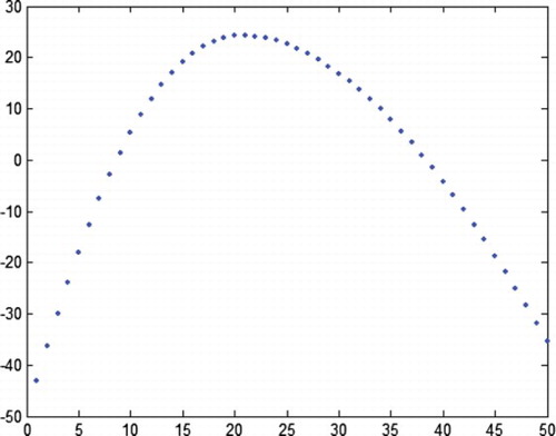
• When p is small (here, p=0.1), all the products within the optimal production lot size should not be inspected, but a partial inspection of the input materials is necessary, i.e. the input materials used for the products produced at the initial parts of the production lot should be inspected. The optimal inspection policy for the products and their input materials is depicted in for γ=1 and in for γ=1.3. Under the optimal inspection policy, the change in the expected total revenue with the different production lot sizes is depicted in for γ=1 and for γ=1.3, where
• When p is large (here p≥0.2), the optimal inspection policy is
Figure 1. The inspection policy when γ=1 and p=0.1.
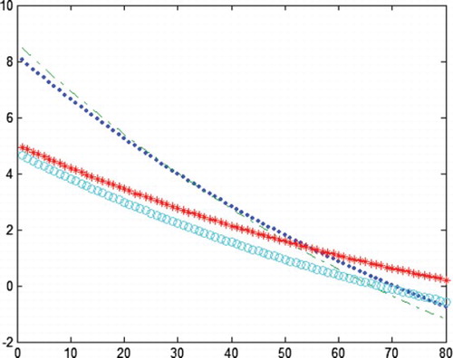
Figure 2. The inspection policy when γ=1.3 and p=0.1.
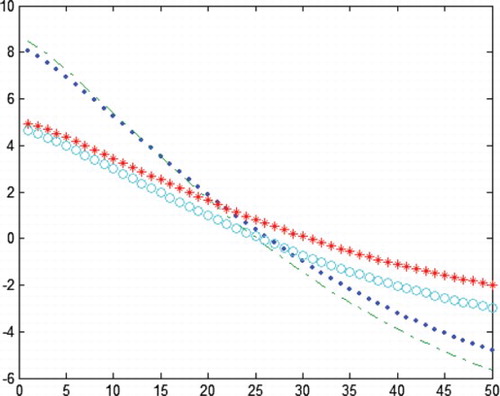
Figure 3. The total revenue versus the production lot size when γ=1 and p=0.1.
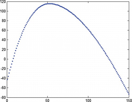
Figure 4. The total revenue versus the production lot size when γ=1.3 and p=0.1.
When p=0.1 and γ=1 (i.e. the process has a geometric shift distribution), the effects of the change of the two types of inspection errors and the values of the model cost parameters on the optimal solution are given in and , respectively, where each time only one parameter value is changed and the other parameters values remain the same.
Table 3. The effects of the inspection errors on the optimal solution (p=0.1 and γ=1).
Table 4. The effects of the various costs on the optimal solution (p=0.1 and γ=1).
shows that when an inspection error increases, both the optimal lot size and the total revenue are non-increasing. When the inspection errors of the input materials, α0 and/or β0, increases, the range of inspection for the input materials dwindles (see the changes in the inspection policy (1,0)). On the other hand, when the inspection errors of the product, α1 and/or β1, increases, the range of product inspection diminishes (see the changes in the inspection policy (0,1)).
Using , one can make the following observations.
• When the unit revenue R′ or the salvaged revenue increases, both the production lot size and total revenue increase. In addition, if R′ and/or S becomes smaller, the no inspection policy for the products and their input materials become preferred, i.e. the range of (0,0) become larger.
• When the cost related to the input material increases, i.e. the replacement cost for an nonconforming material
• On the other hand, when the cost related to the product increases (i.e. the unit nonconforming cost c′d or the unit product inspection cost
5. Conclusions
In this paper, an integrated inspection and lot-sizing model is proposed. We first develop an optimal inspection policy that maximizes the expected total revenue for a given production lot size, where the inspection problem is to decide whether to inspect the jth product and its associated input material. From Proposition 1, one knows that the input materials should be inspected when they are used to produce products during the initial segment of the production lot, and that the products produced at the tail part of the production lot should also be inspected. However, for the middle part of the production lot, both the products and the input materials used should be either inspected or not inspected. In addition, we have explored the conditions related to the adequacy of using Porteus's (Citation1986) lot-sizing model, where both the products and their input materials are not inspected in a production lot. Under the optimal inspection policy, the optimal production lot size can be uniquely determined. In addition, we also explored the conditions for the optimal production lot size. When the process has a geometric shift distribution with a small shift rate, an approximated solution of the optimal production lot size is obtained as a closed-form expression. The illustrated numerical examples demonstrate that a smaller production lot size is required when the used input materials have a higher nonconforming probability and/or when the process has a worse reliability. In addition, when the nonconforming probability of the input material is small enough, one can ignore product inspection but one should still perform a partial inspection of the input materials used to produce the products during the initial part of the production lot.
The authors would like to express our appreciation of the two anonymous reviewers and their valuable comments on this paper. This research was supported by the National Science Council of Taiwan under Grant NSC 100-2410-H-251-007.
REFERENCES
- Avinadav, T., & Raz, T. (2003). Economic optimization in a fixed sequence of unreliable inspections. Journal of the Operational Research Society, 54, 605–613. doi: 10.1057/palgrave.jors.2601543
- Djamaludin, I., Murthy, D. N. P., & Wilson, R. J. (1994). Quality control through lot sizing for items sold with warranty. International Journal of Production Economics, 33, 97–107. doi: 10.1016/0925-5273(94)90123-6
- Hu, F., & Zong, Q. (2009). Optimal production run time for a deteriorating production system under an extended inspection policy. European Journal of Operational Research, 196, 979–986. doi: 10.1016/j.ejor.2008.05.008
- Nakagawa, T., & Osaki, S. (1975). The discrete Weibull distribution. IEEE Transactions on Reliability, R-24(5), 300–301. doi: 10.1109/TR.1975.5214915
- Porteus, E. L. (1986). Optimal lot sizing, process quality improvement and setup cost reduction. Operations Research, 34, 137–144. doi: 10.1287/opre.34.1.137
- Raz, T., Herer, Y. T., & Grosfeld-Nir, A. (2000). Economic optimization of off-line inspection. IIE Transactions, 32, 205–217.
- Sheu, S. H., Chen, Y. C., Wang, W. Y., & Shin, N. H. (2003). Economic off-line inspection with inspection errors. Journal of the Operational Research Society, 54, 888–895. doi: 10.1057/palgrave.jors.2601582
- Tagaras, G., & Lee, H. L. (1996). Economic models for vendor evaluation with quality cost analysis. Management Science, 42(11), 1531–1543. doi: 10.1287/mnsc.42.11.1531
- Tzimerman, A., & Herer, Y. T. (2009). Off-line inspections under inspection errors. IIE Transactions, 41, 626–642. doi: 10.1080/07408170802331250
- Wang, C. H. (2007). Economic off-line quality control strategy with two types of inspection errors. European Journal of Operational Research, 179(1), 132–147. doi: 10.1016/j.ejor.2006.03.024
- Wang, C. H., Dohi, T., & Tsai, W. C. (2010). Coordinated procurement/inspection and production model under inspection errors. Computers and Industrial Engineering, 59(3), 473–478. doi: 10.1016/j.cie.2010.06.008
- Wang, C. H., & Sheu, S. H. (2001). Simultaneous determination of the optimal production-inventory and product inspection policies for a deteriorating production system. Computers and Operations Research, 28, 1093–1110. doi: 10.1016/S0305-0548(00)00030-7
- Wang, C. H., & Sheu, S. H. (2003). Optimal lot sizing for products sold under free-repair warranty. European Journal of Operational Research, 149, 131–141. doi: 10.1016/S0377-2217(02)00429-0
Appendix 1. A proof of Proposition 1(a)
From DRs 1, 4 and 6, we know that for
, and
is never optimal for
. Similarly, from DRs 2, 5 and 6, we know that
for
, and
is never optimal for
j6+1). Also note that
. The above imply that
is either (0,0) or (1,1) for
j6+1). Furthermore, in DR 3-1, it is easy to see that
When p>λ, we have
for
j5+1, j6+1) and
for
.
A similar approach can be used for the remaining cases given in Proposition 1, which are omitted here.
Appendix 2
When p<λ, one has
Appendix 3. A proof of Proposition 2
We first show that decreases when j increases. For a fixed inspection policy, (0,0), (1,0), (0,1) or (1,1), from Equation (9), it is easy to see that the jth product whose expected revenue decreases when j increases.
Suppose that Ij*=x, Kj*=y and Ij+1*=x′, Kj+1*=y′, where or 1, one has
This shows that
is decreasing when j is increasing.
Now, we show the property of n* as follows. It is easy to see that a local maximal solution should satisfy the following two inequalities:
and
On the other hand, when and
<B, since
is decreasing in j, Equation (A4) can be uniquely satisfied. Therefore, the solution to Equation (A4) is the unique optimal solution. In addition, when
, which implicates that
, one has
for n=1, 2, 3, … . This indicates that n*=∞.
Appendix 4