Plankton nutrient interaction model with effect of toxin in presence of modified traditional Holling Type II functional response

Abstract

A three-dimensional plankton-nutrient interaction model is proposed and analysed which mediated by a toxin-determined functional response. The new functional response is a modification of the traditional Holling Type II functional response by explicitly including a reduction in the consumption of phytoplankton by the zooplankton due to chemical defenses. Our analysis leads to different thresholds in terms of model parameters to find out different steady-states behaviour. It is found that constant nutrient input and dilution rate of nutrient influence the plankton ecosystem model and maintain stability around the coexistent equilibrium. Our observations indicate that if the constant nutrient input crosses a certain critical value, the system enters into Hopf bifurcation. In addition, we have studied the direction of Hopf bifurcation by applying the normal form method. The maximal amount of toxin of phytoplankton species plays a crucial role to change the steady-state behaviour. Computer simulations illustrate the results.

Keywords:

• Nutrient
• plankton
• toxin
• stability
• equilibria

1. Introduction

In all marine ecosystems, the interactions between nutrient and plankton are important. These interactions are partially understood due to their complexities. Several scientists have discussed the role of competition in phytoplankton population for the occurrence and control of plankton bloom and the effect of toxin on nutrient-phytoplankton–zooplankton (NPZ) model (Bairagi, Pal, Chatterjee, and Chattopadhyay, 2008; Chakraborty, Bhattacharya, Feudel, and Chattopadhyay, 2012; Chatterjee, Pal, and Chatterjee, 2011; Mukhopadhyay and Bhattacharyya, 2005; Pal, Chatterjee, and Chattopadhyay, 2007). The adverse effect on plankton ecosystem model and downward movement of the equilibrium level of zooplankton biomass due to presence of toxin have been examined by Khare, Misra, and Dhar (2010). As stated by Banerjee and Venturino (2011), the toxic phytoplankton don't lead the zooplankton population to become extinct in plankton marine ecosystem. Jang, Baglama, and Rick (2006) investigated that when phytoplankton and zooplankton can uptake toxin separately, the growth rates of plankton population decrease. But Chattopadhyay, Sarkar, and Pal (2004) showed that there may not be release of toxic chemicals by all the plankton species. Ruan (1993, 2001) has pointed out the importance of nutrient for growth of plankton population in phytoplankton–zooplankton interaction model. The effects of multi nutrient and harmful algal bloom on NPZ model have been investigated by some researchers with variable outcomes (Mitra, 2006; Mitra and Flynn, 2006). The role of delay on plankton ecosystem in the presence of a toxin producing phytoplankton has been examined by Khare, Misra, Singh, and Dhar (2011). This study has also shown the effect of delay in the digestion of nutrient by phytoplankton biomass. In a phytoplankton–zooplankton-fish model with fish affecting the migrations of zooplankton, in turn affects the migrations of motile phytoplankton, as studied by Samanta, Chowdhury, and Chattopadhyay (2013).

Intake of forage is raised by the nutrient (nitrogen, phosphorous, carbohydrates, etc.) as herbivores require them and often are limiting in food supply. The herbivores either stops eating poisonous food or die, as by satiating the detoxification system of herbivores, herbivory is reduced by toxins (Li, Feng, Swihart, Bryant, and Huntly, 2006). Consumption of toxic food stops before the occurrence of lethal poisoning and hence poisoning is not so common. The zooplankton functional response, the linker of zooplankton to phytoplankton population, is a key component in phytoplankton–zooplankton interaction model. The instantaneous change in the rate of prey intake by herbivore in response to changing prey biomass is referred as the said functional response. Holling Type II response, featured by a monotonic increase in intake and asymptotic towards a maximum rate of biomass consumption, is a commonly used functional response. The traditional Holling type II functional response assuming the growth rate of herbivore as a monotonically increasing function of plant density is one of the most commonly used descriptions of the plant consumption by herbivores (Liu, Feng, Zhu, and L DeAngelis, 2008).

However, this will not be appropriate if the chemical defense of phytoplankton is considered, where the negative effect of phytoplankton toxin on zooplankton can lead to a decrease in the growth rate when the phytoplankton density is high. The Holling Type II functional responses is characterized by a monotonic increase in phytoplankton consumption as phytoplankton biomass increases asymptotically towards a maximum consumption rate, at which the zooplankton is satiated. To examine the effect of toxicity on feeding rates, we constructed a simple toxin-determined functional response model (TDFRM) with phytoplankton–zooplankton species.

The toxin-determined functional response is a modification of the traditional Holling Type II response to include the negative effect of toxin on zooplankton growth, which can overwhelm the positive effect of biomass ingestion at sufficiently high phytoplankton toxicant concentrations. The model adds one parameter to the Holling Type 2 response; , which describes the negative effect that phytoplankton toxins have on the zooplankton population's time-dependent per capita intake of phytoplankton biomass. This addition allows one to dynamically model how toxin-determined zooplankton affects when it consumes toxic phytoplankton in plankton dynamics. Thus, the model is a potential tool for resource managers working in ecosystems containing toxic phytoplankton.

As observed by Swihart, L DeAngelis, Feng, and Bryant (2009), three analytical modifications should be considered when incorporating the effects of toxins on plant-herbivore dynamics. Toxin-mediated functional responses should (a) explicitly account for the negative effects of phytoplankton toxins on zooplankton growth; (b) permit herbivores to regulate intake of toxins; and (c) allow for intake of multiple phytoplankton that are detoxified with independent pathways.

Here an open system is considered with three interacting components consisting of phytoplankton (P), zooplankton(Z) and dissolved limiting nutrient (N). In this paper a nutrient-phytoplankton-zooplankton model with the effect of toxin producing phytoplankton is described. The stability of equilibrium point is described. We have also derived the conditions for instability of the system around the interior equilibrium and direction of Hopf bifurcation. Numerical simulations under a set of parameter values have been performed to support our analytical result.

2. Formulation of the mathematical model

Let be the concentration of the nutrient at time t. In addition, P(t) and Z(t) be the concentration of phytoplankton and zooplankton population, respectively, at time t. be the constant input of nutrient concentration, D is the dilution rate of nutrient (Fredrickson and Stephanopoulos, 1981). The constant has the physical dimension of a time and represents the average time that nutrient and waste products spend in the system (Smith, 1981). Let and be the nutrient uptake rate for the phytoplankton population and conversion rate of nutrient for the growth of phytoplankton population, respectively (). is the rate of encounter per unit of phytoplankton species. The parameter is the resource encounter rate, which depends on the movement velocity of the zooplankton and its radius of detection of food items. The parameter () is the fraction of food biomass encountered that the zooplankton ingests, while h is the handling time per unit biomass, which incorporates the time required for the digestive tract to handle the item.

The second part of the toxin determined functional response, that is, , accounts for the negative effect of toxin, where . The parameter is a measure of the maximum amount of toxicant per unit time that the zooplankton can tolerate, and is the amount of toxin per unit phytoplankton biomass. decreases when the concentration of toxin tolerated by the zooplankton decreases (high toxicity) or the concentration of toxin in the phytoplankton biomass increases. Therefore, the smaller the value of , the larger the effect the toxin has on intake.

If we assume that is the same for all individuals within a zooplankton population, then the variation in will result from the different values of of the phytoplankton species encountered. The factor 4 is just a multiplier that simplifies the form of the peak value of as a function of P. Let be the mortality rate of the phytoplankton population and be the mortality rate of the zooplankton population. Let be the maximal zooplankton conversion rate. We have considered Holling type II functional response to describe the grazing phenomena with as half saturation constant.

Now following the above assumption, we consider the mathematical model (1) where (2) We take the initial conditions for the system (1(1) ) as (3)

3. Some preliminary results

3.1. Positive invariance

Due to the constant supply of nutrients , the system (1(1) ) is not homogeneous. By considering and , with and , the system (1(1) ) becomes (4) together with . It is easy to verify that whenever choosing with , for i=1,2,3, then . Then any solution of Equation (4(4) ) with , say , is such that for all t>0. This ensures that the solution remains within the positive orthant, ensuring the biological well-posedness of the system.

3.2. Boundedness of the system

Theorem 1.

All the solutions of (1(1) ) are bounded.

The proof is obvious.

3.3. Equilibria

The system (1(1) ) possesses the following equilibria:

1. The plankton free equilibrium .

2. The zooplankton free equilibrium with and which is exist for .

3. For positive interior equilibrium , we calculate third equation of system (1(1) ) by putting zero in right hand side we get Let and .

   • Case 1: If A>0, B>0, the above quadratic equation has no positive real roots.

   • Case 2: If A<0, B>0, the quadratic equation has one positive real root.

   • Case 3: If A<0, B<0, the quadratic equation has one positive real root.

For Case 2 and Case 3, we get unique positive real root . Then the value of

Thus the conditions for the existence of the unique interior equilibrium point are given by, with (5) and (6)

Case 4: If A>0, B<0, the quadratic equation has two positive real roots.

Let . The maximum value of the function is . Then if A>0 which implies , that is, . Also B<0, if . Combining two conditions we get (7) Then

3.4. Criterion for the extinction of phytoplankton

Theorem 2.

Let the inequality (8) hold. Then .

Theorem (2) demonstrates that if the ratio of maximal nutrient conversion rate for the growth of phytoplankton and the loss rate of the phytoplankton is less than unity then the phytoplankton population will eliminate from the system. The proof is obvious and hence omitted.

3.5. Eigenvalue analysis

In this section, we investigate the local stability behaviour of the system (1(1) ) around each of the equilibria by computing the jacobian matrix. Let be any arbitrary equilibrium. Then the jacobian matrix for is given by

Lemma 1.

The plankton free steady-state of the system (1(1) ) is unstable if .

Proof.

By computing the jacobian matrix for the equilibrium of the system (1(1) ) we get three eigenvalues like , and , where . Clearly is asymptotically stable if and only if . When , plankton free steady state is unstable and a feasible zooplankton free steady-state exists.

Lemma 2.

There exists a feasible zooplankton free steady-state of the system (1(1) ) which is unstable if (9)

Proof.

Further the eigenvalues of the jacobian matrix around the equilibrium of the system (1(1) ) are , which are the roots of the equation and , where . Clearly and have negative real parts because all the coefficients of above quadratic equation is positive. Therefore if condition (9(9) ) is satisfied and hence is unstable.

We summarized the analytical results in Table 1.

Table 1. The table representing thresholds and stability of steady states.

Thresholds()	()	()	()
	Asymptotically stable	Not feasible	Not feasible
	Unstable	Asymptotically stable	Not feasible
	Unstable	Unstable	Asymptotically stable

Stability analysis of the positive interior equilibrium of the system (1(1) ).

The jacobian matrix of system (1(1) ) around the positive equilibrium is where The characteristic equation is (10) where

Now if .

Here if .

Also if . Finally, if . Then the system becomes locally asymptotically stable around . Thus depending upon system parameters, the system may exhibit stable or unstable behaviour in this case.

Remark 1.

The system could have a Hopf-bifurcation at the coexistence equilibrium if the following two conditions are satisfied, (11)

3.6. Hopf bifurcation at coexistence

In fact, the bifurcation occurs when the characteristic Equation (10(10) ) has to have two purely imaginary roots , where denotes the imaginary unit, in addition to the real one e. It follows that it can be rewritten as . Expanding, we find . Comparing the coefficients with those of Equation (10(10) ) the first condition (11(11) ) follows. The transversality condition, the second (11(11) ), is obtained observing that the eigenvalues of the characteristic equation, of the form must satisfy the transversality condition . Substituting into the characteristic equation, separating the real and imaginary parts and eliminating η, using for shorthand, we get Differentiating this cubic with respect to , we find At , we have , so that the above equation becomes providing the second condition (11(11) ). This ensures that the system (1(1) ) has a Hopf-bifurcation around the positive interior equilibrium .

An analytic verification of Equation (11(11) ) appears in these conditions a very difficult task, as the coefficients depend on the population levels at equilibrium . However, these remarks help in guiding the numerical simulations, that in fact reveal the existence of sustained population oscillations.

Theorem 3.

The parameter determines the direction of the Hopf-bifurcation. If () then the Hopf-bifurcation is supercritical (subcritical) and the bifurcating periodic solutions exists for .

The stability and the period of the bifurcating periodic solutions are, respectively, determined by the parameters and defined in the proof. The solutions are orbitally stable (unstable) if () and the period increases (decreases) if ().

Proof.

We just outline the sketch of the proof, because the computational details are very complicated. The method is based on the normal form theory (Hassard, Kazarinoff, and Wan, 1981). In the conditions of the Hopf bifurcation given in the above Remark 1, let us denote by a bar the system parameters; the eigenvector corresponding to the eigenvalue is

The eigenvector corresponding to the eigenvalue e is Let us define the following quantities: Using the transformation system (1(1) ) is then reduced to (12) where as a shorthand we have introduced the following quantities: The equilibrium point of the new system (12(12) ) is now the origin. At it, the Jacobian of (12(12) ) simplifies since several entries vanish: Further, the following auxiliary quantities can be explicitly calculated in terms of the system parameters, but we omit the explicit formulae in view of their excessive length.

The values of and , obtained from (Hassard et al., 1981; Sen, Mukherjee, Giri, and Das, 2011), can now be calculated from the above quantities, Recalling finally (Hassard et al., 1981), if the root of the characteristic equation increases for increasing values of the bifurcation parameter , namely , the periodic solution emanating from the equilibrium for is supercritical while it is subcritical for .

4. Numerical simulations

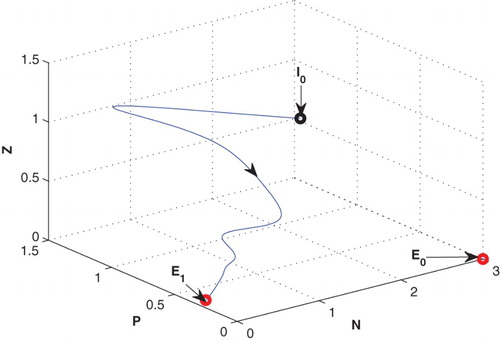
In this section, we focus our attention on the occurrence and termination of the fluctuating plankton population. We begin with a parameter set (see Table 2, reference Feng, Qiu, Liu, and L DeAngelis, 2011) for which the existence criterion at equilibrium of coexistence is satisfied. In this case coexistence equilibrium point is locally asymptotically stable in the form of a stable focus (cf. Figure 1).

Figure 1. The equilibrium point is stable for the parametric values as given in Table 2.

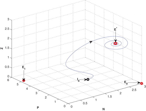
Table 2. A set of parametric values.

	Constant input of nutrient	3
D	Dilution rate of nutrient	0.3
	Nutrient uptake rate for the phytoplankton	0.9
	Nutrient conversion rate for the phytoplankton	0.8
	Rate of encounter per unit of phytoplankton species	0.3
	Fraction of effort applied to foraging for plankton species	0.7
h	Handling time of the zooplankton	0.3
	Max units of phytoplankton species a zooplankton can eat per day	3
	Conversion constant (zooplankton species per unit phytoplankton species)	0.5
	Half saturation constant for phytoplankton	0.6
	Mortality rate of phytoplankton	0.15
	Mortality rate of zooplankton	0.04

4.1. Effects of

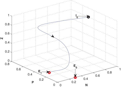
Increasing the value of constant nutrient input from 3 to 5.5, the equilibrium switches from stable to oscillatory behaviour around the for same set of parametric values in Table 2 (cf. Figure 2). But in presence of low value of constant nutrient input, , system goes to zooplankton free equilibrium (cf. Figure 3).

Figure 2. The figure depicts oscillatory behaviour around the positive interior equilibrium of the system (2.1) for increasing from 3 to 5.5 with same set of parametric values as given in Table 2.

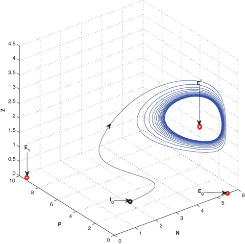
Figure 3. The figure depicts stable behaviour at of the system (2.1) for with same set of parametric values as given in Table 2.

4.2. Effects of D

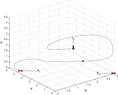
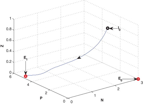
For D=0.85, leaving all other parameters unaltered, the system exhibits oscillation around the positive interior equilibrium (cf. Figure 4). But decreasing the value of D from 0.3 to 0.02, the system goes to zooplankton free equilibrium (cf. Figure 5).

Figure 4. The figure depicts oscillatory behaviour around the positive interior equilibrium of the system (2.1) for increasing D from 0.3 to 0.85 with same set of parametric values as given in Table 2.

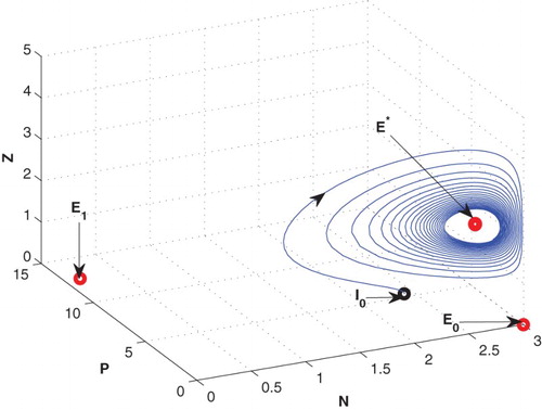
Figure 5. The figure depicts stable behaviour at of the system (2.1) for D=0.02 with same set of parametric values as given in Table 2.

4.3. Effects of

We have observed that the system shows oscillatory behaviour around the positive interior equilibrium for low value of (cf. Figure 6). If is further decreasing from 0.25 to 0.15, the system becomes stable at zooplankton free equilibrium in the form of a stable focus (cf. Figure 7).

Figure 6. The figure depicts oscillatory behaviour around the positive interior equilibrium of the system (2.1) for decreasing the value of from 3 to 0.25 with same set of parametric values as given in Table 2.

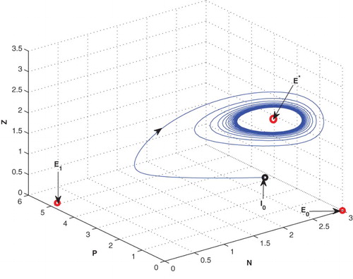
Figure 7. The figure depicts stable behaviour at of the system (2.1) for G₁=0.15 with same set of parametric values as given in Table 2.

4.4. Effect of

If the mortality rate of zooplankton is increased from 0.04 to 0.4, the system goes to zooplankton free equilibrium at (cf. Figure 8).

Figure 8. The figure depicts stable behaviour at of the system (2.1) for increasing the value of with same set of parametric values as given in Table 2.

4.5. Hopf-bifurcation

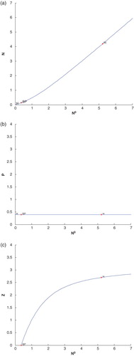
System behaviour can be demonstrated more prominently if we plot the bifurcation diagram for constant nutrient input, , as a bifurcation parameter with other three species. Here we see a Hopf bifurcation at with first Lyapunov coefficient (cf. Figure 9(a)–(c). Clearly the value of first Lyapunov coefficient is negative. This means that a stable limit cycle bifurcates from the equilibrium, when it looses stability. In Figure 9(a)–(c), , known as branch point, H (right side of BP) denotes Hopf bifurcation point and H (left side of BP) denotes neutral saddles which are not bifurcation points.

Figure 9. (a) The figure depicts different steady-state behaviour of nutrient for the effect of . (b) The figure depicts different steady-state behaviour of phytoplankton for the effect of . (c) The figure depicts different steady-state behaviour of zooplankton for the effect of with other parametric values as given in Table 2.

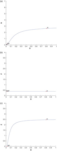
We have plotted another diagram with dilution rate of nutrient, D, with other three species (cf. Figure 10(a)–(c)). Again we see that a Hopf bifurcation occurs at D=0.807954 with first Lyapunov coefficient is . This means that a stable limit cycle bifurcation from the equilibrium, when it looses stability. In Figure 10(a)–(c), , known as branch point, H (right side of BP) denotes Hopf bifurcation point and H (left side of BP) denotes neutral saddles which are not bifurcation points.

Figure 10. (a) The figure depicts different steady-state behaviour of nutrient for the effect of D. (b) The figure depicts different steady-state behaviour of phytoplankton for the effect of D. (c) The figure depicts different steady-state behaviour of zooplankton for the effect of D with other parametric values as given in Table 2.

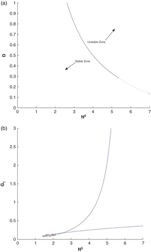
Next we have plotted a two parameters bifurcation diagram for showing a clear picture of stable and unstable zone in this system (cf. Figure 11(a)). Finally, we have plotted a two parameters bifurcation diagram, . Here we see a generalized Hopf (GH) point, where the first Lyapunov coefficient vanishes but the second Lyapounov coefficient is non-zero. The bifurcation point separates branches of sub and supercritical Andronov–Hopf bifurcations in the parameter plain. The Bogdanov–Takens (BT) point is common point for the limit point curve and the curve corresponding to equilibria. The system has an equilibrium with a double zero eigenvalues at BT point. For nearby parameter values, the system has two equilibria (a saddle and a non-saddle ) which collide and disappear via a saddle-node bifurcation. The non-saddle equilibrium undergoes an Andronov–Hopf bifurcation generating a limit cycle (cf. Figure 11(b)).

Figure 11. (a) The two parameter bifurcation diagram for –D with all parametric values as given in Table 2 of the system (2.1). (b) The two parameter bifurcation diagram for – with all parametric values as given in Table 2 of the system (2.1).

5. Discussion

A nutrient-plankton interaction model in presence of toxin producing phytoplankton is considered with Holling type II nutrient uptake function. We study the dynamics of the system (1(1) ) with a functional response mediated by phytoplankton toxicity. This toxin-determined functional response model (TDFRM) is a modification of the traditional consumer resource model with Holling Type II functional response. Firstly, The model is studied analytically and the threshold conditions for the existence and stability of various steady states are worked out, see Table 1. Note that our recent model is different from other models (Feng et al., 2011; Li et al., 2006; Liu et al., 2008). Our discussion has focused on nutrient-plankton ecosystem apart from plant-herbivore system. Recent modelling efforts implicate nutrient input as potentially key drivers of change in plankton ecosystem. The simulation result confirmed the existence of a stable periodic solution when the stable interior equilibrium loses its stability. It is observed that there is a chance for the fluctuating population for high value of constant nutrient input. Thus, our analysis shows that if the constant nutrient input crosses a critical value, say , the system (1(1) ) enters into Hopf bifurcation that induces stable limit cycle periodic solutions around the positive equilibrium. Then all the populations start to oscillate. But for low values of constant nutrient input it may lead to extinction of zooplankton population. Moreover, change in stability of interior equilibrium is demonstrated using several key parameters including the dilution rate of nutrient, mortality rate of zooplankton and phytoplankton toxicity.

Our simulations also helped us to indicate that, in presence of high dilution rate of nutrient there is chance for oscillatory behaviour of plankton population. But at low value of dilution rate of nutrient, zooplankton goes to extinction.

Also our observation indicates that there is a chance for oscillatory behaviour in presence of low value of toxicity level of phytoplankton species. Further, decreasing the value of toxicity level of phytoplankton species, the zooplankton goes to extinction. Similar case arises for high value of mortality rate of zooplankton population.

Thus our analysis suggests that to control the fluctuating population and to maintain stability around the coexistence of equilibrium, we have to control the constant nutrient input, dilution rate of nutrient and toxicity level of phytoplankton population.

Acknowledgments

The paper has improved considerably, both in presentation and scientific content, by the critical comments made by the reviewers. The authors are thankful to them. Authors are also thankful to Professor Zidong Wang, Executive Editor, System Science and Control Engineering, for his valuable comments.

Disclosure Statement

No potential conflict of interest was reported by the authors.

ORCID

Samares Pal http://orcid.org/0000-0002-8792-0031

Additional information

Funding

Research is supported by DST (PURSE Scheme), University Kalyani, India. The research is partially supported by University Grants Commission, New Delhi [grant number MRP-MAJ-MATH-2013-609].

References

- Bairagi, N., Pal, S., Chatterjee, S., & Chattopadhyay, J. (2008). Nutrient, non-toxic phytoplankton, toxic phytoplankton and zooplankton interaction in the open marine system. In R. J. Hosking & E. Venturino (Eds.), Aspects of mathematical modelling, mathematics and biosciences in interaction (pp. 41–63). Basel: Birkhauser Verlag.
- Banerjee, M., & Venturino, E. (2011). A phytoplankton-toxic phytoplankton–zooplankton model. Ecological Complexity, 8(3), 239–248.
- Chakraborty, S., Bhattacharya, S., Feudel, U., & Chattopadhyay, J. (2012). The role of avoidance by zooplankton for survival and dominance of toxic phytoplankton. Ecological Complexity, 11, 144–153.
- Chatterjee, A., Pal, S., & Chatterjee, S. (2011). Bottom up and top down effect on toxin producing phytoplankton and its consequence on the formation of plankton bloom. Applied Mathematics and Computation, 218(7), 3387–3398.
- Chattopadhyay, J., Sarkar, R. R., & Pal, S. (2004). Mathematical modelling of harmful algal blooms supported by experimental findings. Ecological Complexity, 1(3), 225–235.
- Feng, Z., Qiu, Z., Liu, R., & LDeAngelis, D. (2011). Dynamics of a plant-herbivore-predator system with plant-toxicity. Mathematical Biosciences, 229(2), 190–204.
- Fredrickson, A. G., & Stephanopoulos, G. (1981). Microbial competition. Science, 213(4511), 972–979.
- Hassard, B. D., Kazarinoff, N. D., & Wan, Y. H. (1981). Theory and application of Hopf bifurcation. Cambridge: Cambridge University Press.
- Jang, S. R.-J., Baglama, J., & Rick, J. (2006). Nutrient-phytoplankton–zooplankton models with a toxin. Mathematical and Computer Modelling, 43, 105–118.
- Khare, S., Misra, O. P., & Dhar, J. (2010). Role of toxin producing phytoplankton on a plankton ecosystem. Nonlinear Analysis: Hybrid Systems, 4(3), 496–502.
- Khare, S., Misra, O. P., Singh, C., & Dhar, J. (2011). Role of delay on planktonic ecosystem in the presence of a toxic producing phytoplankton. International Journal of Differential Equations. doi:10.1155/2011/603183.
- Li, Y., Feng, Z., Swihart, R., Bryant, J., & Huntly, N. (2006). Modeling the impact of plant toxicity on plant-herbivore dynamics. Journal of Dynamics and Differential Equations, 18(4), 1021–1042.
- Liu, R., Feng, Z., Zhu, H., & L DeAngelis, D. (2008). Bifurcation analysis of a plant-herbivore model with toxin-determined functional response. Journal of Differential Equations, 245(2), 442–467.
- Mitra, A. (2006). A multi-nutrient model for the description of stoichiometric modulation of predation in micro- and mesozooplankton. Journal of Plankton Research, 28(6), 597–611.
- Mitra, A., & Flynn, K. J. (2006). Promotion of harmful algal blooms by zooplankton predatory activity. Biology Letters, 2(2), 194–197.
- Mukhopadhyay, B., & Bhattacharyya, R. (2005). A delay-diffusion model of marine plankton ecosystem exhibiting cyclic nature of blooms. Journal of Biological Physics, 31(1), 3–22.
- Pal, S., Chatterjee, S., & Chattopadhyay, J. (2007). Role of toxin and nutrient for the occurrence and termination of plankton bloom – results drawn from field observations and a mathematical model. BioSystems, 90, 87–100.
- Ruan, S. (1993). Persistence and coexistence in zooplankton–phytoplankton-nutrient models with instantaneous nutrient recycling. Journal of Mathematical Biology, 31(6), 633–654.
- Ruan, S. (2001). Oscillations in plankton models with nutrient recycling. Journal of Theoretical Biology, 208, 15–26.
- Samanta, S., Chowdhury, T., & Chattopadhyay, J. (2013). Mathematical modeling of cascading migration in a tri-trophic food-chain system. Journal of Biological Physics, 39(3), 469–487.
- Sen, A., Mukherjee, D., Giri, B. C., & Das, P. (2011). Stability of limit cycle in a prey–predator system with pollutant. Applied Mathematical Science, 5(21), 1025–1036.
- Smith, H. L. (1981). Competitive coexistence in an oscillating chemostat. SIAM Journal on Applied Mathematics, 4, 498–522.
- Swihart, R. K., L DeAngelis, D., Feng, Z., & Bryant, P. J. (2009). Troublesome toxins: Time to re-think plant-herbivore interactions in vertebrate ecology. BMC Ecology. doi:10.1186/1472-6785-9-5.