The paradigm of complex probability and Chebyshev’s inequality

ABSTRACT

The system of axioms for probability theory laid in 1933 by Andrey Nikolaevich Kolmogorov can be extended to encompass the imaginary set of numbers and this by adding to his original five axioms an additional three axioms. Therefore, we create the complex probability set , which is the sum of the real set with its corresponding real probability, and the imaginary set with its corresponding imaginary probability. Hence, all stochastic experiments are performed now in the complex set instead of the real set . The objective is then to evaluate the complex probabilities by considering supplementary new imaginary dimensions to the event occurring in the ‘real’ laboratory. Consequently, the corresponding probability in the whole set is always equal to one and the outcome of the random experiments that follow any probability distribution in is now predicted totally in . Subsequently, it follows that, chance and luck in is replaced by total determinism in . Consequently, by subtracting the chaotic factor from the degree of our knowledge of the stochastic system, we evaluate the probability of any random phenomenon in . This novel complex probability paradigm will be applied to the established theorem of Pafnuty Chebyshev's inequality and to extend the concepts of expectation and variance to the complex probability set .

KEYWORDS:

• Complex set
• probability norm
• degree of our knowledge
• chaotic factor
• complex random vector
• resultant complex random vector
• complex expectation and variance

Nomenclature

	=	= real set of events
	=	= imaginary set of events
	=	= complex set of events
i	=	= the imaginary number where
Prob	=	= probability of any event
Pr	=	= probability in the real set
Pm	=	= probability in the imaginary set corresponding to the real probability in
Pc	=	= probability of an event in with its associated event in , it is the probability in the complex set
z	=	= complex number = sum of Pr and Pm = complex random vector
	=	= = the degree of our knowledge of the random experiment, it is the square of the norm of z.
Chf	=	= the chaotic factor of z
MChf	=	= magnitude of the chaotic factor of z
N	=	= number of random variables
Z	=	= the resultant complex random vector
	=	= probability in Z in the real set
	=	= probability in Z in the imaginary set corresponding to the real probability in
	=	= probability in Z in the complex set
	=	= = the degree of our knowledge of Z
	=	= the chaotic factor of Z
	=	= magnitude of the chaotic factor of Z
Er	=	= expectation in the real set
Em	=	= expectation in the imaginary set
Ec	=	= expectation in the complex set
Vr	=	= variance in the real set
Vm	=	= variance in the imaginary set
Vc	=	= variance in the complex set

1. Introduction

One of the branches of mathematics is the probability theory, which is devoted to probability and to the analysis of random phenomena. Random variables, stochastic processes and events are the fundamental entities of the theory of probability, and which are mathematical abstractions of non-deterministic events or measured quantities that may either be single occurrences or evolve over time in an apparently random fashion (Kuhn, 1970; Poincaré, 1968; Stewart, 1996). According to the classical probability theory, the results of random events cannot be predicted precisely. However, certain patterns which can be studied and predicted are exhibited in a sequence of individual events such as coin flipping or the roll of dice that are influenced by other factors such as friction. The law of large numbers and the central limit theorem are two mathematical results that describe such stochastic patterns (Barrow, 1992; Stewart, 2012; Warusfel & Ducrocq, 2004).

Moreover, probability theory, which is an essential foundation of the field of mathematical statistics, is indispensable to many human activities that involve quantitative analysis of large sets of data. In statistical mechanics, where the descriptions of complex systems are given a partial knowledge of their state, we apply the methods of the classical probability theory. The probabilistic nature of physical phenomena at atomic scales which are described in quantum mechanics is an illustrious discovery of the twentieth century physics (Greene, 2003; Hawking, 2005; Penrose, 1999). Compared to geometry for example, the classical theory of probability as a mathematical subject arose very late, despite the fact that we have prehistoric evidence of man playing with dice from cultures from all over the world. Additionally, Gerolamo Cardano was one of the earliest writers on probability and the earliest known definition of classical probability was perhaps produced by him (Bogdanov & Bogdanov, 2010, 2012, 2013).

Furthermore, in the seventeenth century, precisely in the year 1654, the eminent mathematician and philosopher Blaise Pascal sustained the development of probability when he had some correspondence with his father's friend, Pierre de Fermat, about two problems concerning games of chance that he had heard from the Chevalier de Méré earlier the same year, whom Pascal happened to accompany during a trip. The famous so-called problem of points is one problem which is a classical problem already then treated by Luca Pacioli as early as 1494 and even earlier in an anonymous manuscript in 1400, and deals with the question how to split the money at stake in a fair way when the game at hand is interrupted half-way through. The other problem was one about a mathematical rule of thumb that seemed not to hold when extending a game of dice from using one die to two dice. This last problem, or paradox, was the discovery of Méré himself and showed, according to him, how dangerous it was to apply mathematics to reality. Other mathematical–philosophical issues and paradoxes were discussed, as well during the trip that Méré thought was strengthening his general philosophical view (Bogdanov & Bogdanov, 2009; Davies, 1993; Wikipedia, Probability Theory). Also, Blaise Pascal disagreed with the Chevalier de Méré who viewed mathematics as something beautiful and flawless but poorly connected to reality, and therefore determined to prove Méré wrong by solving these two problems within pure mathematics. When Pascal learned that Pierre de Fermat, already recognized as a distinguished mathematician, had reached the same conclusions, he was convinced that they had solved the problems conclusively. Other scholars at the time – in particular, Huygens, Roberval and indirectly Caramuel – knew about this circulated correspondence, which marks the starting point for when mathematicians in general began to study problems from games of chance. Knowing that, the correspondence did not mention ‘probability’; it focused on fair prices (Wikipedia, Probability Distribution, Probability Density Function, Probability Space).

In addition, the famous mathematician Bernoulli, half a century later, showed a sophisticated grasp of probability. He showed, in fact, facility with permutations and combinations and discussed the concept of probability with examples beyond the classical definition, such as personal, judicial, and financial decisions, and showed that probabilities could be estimated by repeated trials with uncertainty diminished as the number of trials increased (Wikipedia, Probability Measure, Probability Axioms, Chebyshev’s Inequality).

Also, in the eighteenth century, precisely in 1765, the illustrious classical volume of the ‘Encyclopédie’ of Denis Diderot and Jean le Rond d'Alembert contained a lengthy discussion of probability and a summary of knowledge up to that time. In the encyclopedia, a distinction is made between probabilities ‘drawn from the consideration of nature itself’ (physical) and probabilities ‘founded only on the experience in the past which can make us confidently draw conclusions for the future’ (evidential). Moreover, in 1657, Christiaan Huygens published a book on the subject, and in the nineteenth century a big work was done by Le Marquis Pierre-Simon de Laplace in what can be considered today as the classical probability interpretation (Hawking, 2011; Wikipedia, Pafnuty Chebyshev, Markov’s Inequality). As a matter of fact, Laplace provided the source of a clear and lasting definition of probability. As late as 1814 he stated:

The theory of chance consists in reducing all the events of the same kind to a certain number of cases equally possible, that is to say, to such as we may be equally undecided about in regard to their existence, and in determining the number of cases favorable to the event whose probability is sought. The ratio of this number to that of all the cases possible is the measure of this probability, which is thus simply a fraction whose numerator is the number of favorable cases and whose denominator is the number of all the cases possible. [Marquis Pierre-Simon de Laplace, A Philosophical Essay on Probabilities (Wikipedia, Probability Theory)]

This classical definition provides what would be the ultimate description of probability. Several editions of multiple documents were published by Laplace (technical and a popularization) on probability over a half-century span. Many of his predecessors such as Cardano, Bernoulli and Bayes published a single document posthumously (Hawking, 2002). Initially, discrete events were mainly considered by probability theory, and its methods were essentially combinatorial. Furthermore, the incorporation of continuous variables into the theory was done due to analytical considerations (Aczel, 2000).

Additionally, Andrey Nikolaevich Kolmogorov laid the foundations of probability theory, which culminated in the twentieth century. Precisely, in 1933, Kolmogorov combined the notion of sample space, introduced by Richard von Mises, and measure theory and presented his axiom system for probability theory. Fairly quickly this became the mostly undisputed axiomatic basis for modern probability theory, knowing that alternatives exist, in particular the adoption of finite rather than countable additivity by Bruno de Finetti (Pickover, 2008).

Moreover, discrete probability distributions and continuous probability distributions are treated separately in most introductions to probability theory. The more advanced ‘measure theory’, which is based on the treatment of probability, covers both the discrete, the continuous, any mix of these two and more. Since they well describe many natural or physical processes, certain random variables occur very often in probability theory. Therefore, their distributions have gained special importance in the classical theory of probability. We mention here some fundamental discrete distributions, which are the discrete uniform, Bernoulli, binomial, negative binomial, Poisson and geometric distributions. In addition, we mention some important continuous distributions, which include the continuous uniform, normal or Gauss–Laplace, exponential, gamma and beta distributions (Reeves, 1988; Ronan, 1988).

I conclude the introduction with two very important citations of two eminent mathematicians and philosophers who inspired me greatly when developing the complex probability paradigm (CPP):

An intellect which at any given moment knew all the forces that animate Nature and the mutual positions of the beings that comprise it, if this intellect were vast enough to submit its data to analysis, could condense into a single formula the movement of the greatest bodies of the universe and that of the lightest atom: for such intellect nothing could be uncertain; and the future just like the past would be present before its eyes. (Marquis Pierre-Simon de Laplace)

The Divine Spirit found a sublime outlet in that wonder of analysis, that portent of the ideal world, that amphibian between being and not-being, which we call the imaginary root of negative unity. (Gottfried Wilhelm Von Leibniz)

Finally, this research paper is organized as follows: After the introduction in Section 1, the purpose and the advantages of the present work are presented in Section 2. Then in Section 3, Chebyshev's inequality is explained. Afterward, in Section 4, I explain and illustrate the CPP, and in Section 5, I apply the new paradigm to Chebyshev's inequality. Moreover, in Section 6, I do numerical simulations of some discrete and continuous distributions to support the new model. Additionally, in Section 7, I link the resultant complex random vector Z to Chebyshev's inequality. Furthermore, in Section 8, I define the complex characteristics of the probability distributions such as the expectation and the variance. Finally, I conclude the work by doing a comprehensive summary in Section 9, and then present the list of references cited in the current research work.

2. The purpose and the advantages of the present work

All our work in classical probability theory is to compute probabilities. The original idea in this paper is to add new dimensions to our random experiment, which will make the work deterministic. In fact, the probability theory is a non-deterministic theory by nature; that means that the outcome of the events is due to chance and luck. By adding new dimensions to the event in , we make the work deterministic and hence a random experiment will have a certain outcome in the complex set of probabilities . It is of great importance that the stochastic system becomes totally predictable since we will be totally knowledgeable to foretell the outcome of chaotic and random events that occur in nature for example in statistical mechanics or in all stochastic processes. Therefore the work that should be done is to add to the real set of probabilities , the contributions of which is the imaginary set of probabilities which will make the event in  =  +  deterministic. If this is found to be fruitful, then a new theory in statistical sciences and prognostic is elaborated and this is to understand deterministically those phenomena that used to be random phenomena in . This is what I called ‘the complex probability paradigm’, which was initiated and elaborated in my six previous papers (Abou Jaoude, El-Tawil, & Kadry, 2010; Abou Jaoude, 2013a, 2013b, 2014, 2015a, 2015b).

Consequently, the purpose and the advantages of the present work are to:

1. Extend classical probability theory to the set of complex numbers, hence to relate probability theory to the field of complex analysis. This task was initiated and elaborated in my six previous papers and will be more developed in this seventh research work.

2. Apply the new probability axioms and paradigm to Chebyshev's inequality; hence, extend Chebyshev's inequality beyond the real probability set to encompass the complex probability set.

3. Prove that all random phenomena can be expressed deterministically in the complex set .

4. Quantify both the degree of our knowledge (DOK) and the chaos of the random variables.

5. Draw and represent graphically the functions and parameters of the novel paradigm associated to Chebyshev's inequality.

6. Apply the new Chebyshev's theorem to very well-known discrete and continuous probability distributions and thus prove its validity when dealing with any distribution not treated in the current research paper.

7. Show that the classical concepts of expectation and variance can be extended to (complex set) =  (real set) +  (imaginary set).

8. Pave the way to apply the original paradigm to other topics in statistical mechanics, in stochastic processes, to the field of prognostics in engineering. These will be the subjects of my subsequent research papers.

In fact, to summarize and to state the framework of this paper, I will apply throughout this whole research work the novel CPP to the established theorem of Chebyshev's inequality and I will extend the concepts of expectation and variance to the complex probability set . The potential applications of this original theorem are in any field related to stochastic processes whether in applied or pure mathematics, in thermodynamics or statistical mechanics or physics in general, or in any field of engineering or science as a whole, when dealing with probability and random phenomena.

3. Pafnuty Chebyshev’s inequality and contribution

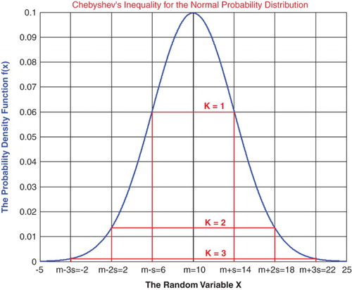
Pafnuty Chebyshev's inequality (also spelled as Tchebysheff's inequality, Russian: ) in probability theory, guarantees that in any probability distribution, ‘nearly all’ values are close to the mean – the precise statement being that no more than 1/k² of the distribution's values can be more than k standard deviations away from the mean (or equivalently, at least 1 − 1/k² of the distribution's values are within k standard deviations of the mean). The rule is often called Chebyshev's theorem, about the range of standard deviations around the mean, in statistics (Wikipedia, Probability Theory, Probability Distribution).

Moreover, because it can be applied to completely arbitrary distributions (unknown except for mean and variance), Chebyshev's inequality has great utility. For example, it can be used to prove the weak law of large numbers (Wikipedia, Probability Density Function, Probability Space).

In practical usage, in contrast to the 68-95-99.7% rule (which applies to normal distributions), under Chebyshev's inequality a minimum of just of values must lie within two standard deviations of the mean and within three standard deviations (Figure 1) (Wikipedia, Probability Measure, Probability Axioms).

Figure 1. Chebyshev's inequality applied to the Normal Probability Distribution.

Additionally, the term Chebyshev's inequality may also refer to Markov's inequality, especially in the context of analysis.

It is important to mention here that the theorem is named after the Russian mathematician Pafnuty Chebyshev, although it was first formulated by his friend and colleague Irénée-Jules Bienaymé. The theorem was first stated without proof by Bienaymé in 1853 and later proved by Chebyshev in 1867. His student Andrey Markov provided another proof in his 1884 Ph.D. thesis (Wikipedia, Chebyshev’s Inequality, Pafnuty Chebyshev, Markov’s Inequality).

In addition, Chebyshev's inequality is usually stated for random variables, but can be generalized to a statement about measure spaces (Ferentinos, 1982; Katarzyna & Dominik, 2010).

Furthermore, let X (integrable) be a random variable with finite expected value μ and finite non-zero variance σ². Then for any real number , we have (1) Only the case where is useful. When the right hand: and the inequality is trivial as all probabilities are . As an example, using shows that the probability that values lie outside the interval does not exceed 1/2 (Baranoski, Rokne, & Xu, 2001; Kabán, 2012).

Because it can be applied to completely arbitrary distributions (unknown except for mean and variance), the inequality generally gives a poor bound compared to what might be deduced if more aspects are known about the distribution involved (Beasley et al., 2004).

To conclude and to summarize, Chebyshev's theorem holds for any distribution of observations and, for this reason, the results are usually weak. The value given by the theorem is a lower bound only. That is, we know that the probability of a random variable falling within two standard deviations of the mean can be no less than 3/4, but we never know how much more it might actually be. Only when the probability distribution is known can we determine exact probabilities. For this reason we call the theorem a distribution-free result. When specific distributions are assumed as in the following sections of this research paper, the results will be less conservative. The use of Chebyshev's theorem is relegated to situations where the form of the distribution is unknown (He, Zhang, & Zhang, 2010).

4 The extended set of probability axioms

4.1 The original Andrey N. Kolmogorov set of axioms

The simplicity of Kolmogorov's system of axioms may be surprising. Let E be a collection of elements {E₁, E₂, … } called elementary events and let F be a set of subsets of E called random events. The five axioms for a finite set E are (Benton, 1966a, 1966b; Feller, 1968; Montgomery & Runger, 2003; Walpole, Myers, Myers, & Ye, 2002):

• Axiom 1: F is a field of sets.

• Axiom 2: F contains the set E.

• Axiom 3: A non-negative real number P_rob(A), called the probability of A, is assigned to each set A in F. We have always 0 ≤ P_rob(A) ≤ 1.

• Axiom 4: P_rob(E) equals 1.

• Axiom 5: If A and B have no elements in common, the number assigned to their union is

• Hence, we say that A and B are disjoint; otherwise, we have

And we say also that P_rob(A∩B) = P_rob(A) × P_rob(B|A) = P_rob(B) × P_rob(A|B), which is the conditional probability. If both A and B are independent, then P_rob(A∩B) = P_rob(A) × P_rob(B).

Moreover, we can generalize and say that for N disjoint (mutually exclusive) event (for ), we have the following additivity rule: And we say also that for N independent events (for ), we have the following product rule:

4.2. Adding the imaginary part

Now, we can add to this system of axioms an imaginary part such that:

• Axiom 6: Let be the probability of an associated event in (the imaginary part) to the event A in (the real part). It follows that , where i is the imaginary number with .

• Axiom 7: We construct the complex number or vector having a norm such that: .

• Axiom 8: Let P_c denote the probability of an event in the universe where  =  + .

• We say that P_c is the probability of an event A in with its associated event in such that

We can see that the system of axioms defined by Kolmogorov could hence be expanded to take into consideration the set of imaginary probabilities by adding three new axioms (Abou Jaoude, 2013a, 2013b, 2014, 2015a, 2015b; Abou Jaoude et al., 2010)

4.3. The purpose of extending the axioms

It is apparent from the set of axioms that the addition of an imaginary part to the real event makes the probability of the event in always equal to 1. In fact, if we begin to see the set of probabilities as divided into two parts, one real and the other imaginary, understanding will follow directly. The random event that occurs in (like tossing a coin and getting a head) has a corresponding probability . Now, let be the set of imaginary probabilities and let be the DOK of this phenomenon. is always, and according to Kolmogorov's axioms, the probability of an event.

A total ignorance of the set makes:

and in this case is equal to: . Conversely, a total knowledge of the set in makes:

and . Here we have because the phenomenon is totally known, that is, its laws and variables are completely determined; hence, our DOK of the system is 1 or 100%.

Now, if we can tell for sure that an event will never occur, that is, like ‘getting nothing’ (the empty set), is accordingly equal to 0, that is the event will never occur in . will be equal to:

, and , because we can tell that the event of getting nothing surely will never occur; thus, the DOK of the system is 1 or 100% (Abou Jaoude et al., 2010).

We can infer that we have always (2) And what is important is that in all cases we have (3) In fact, according to an experimenter in , the game is a game of chance: the experimenter does not know the output of the event. He will assign to each outcome a probability and he will say that the output is non-deterministic. But in the universe  =  + , an observer will be able to predict the outcome of the game of chance since he takes into consideration the contribution of , so we write Hence is always equal to 1. In fact, the addition of the imaginary set to our random experiment resulted in the abolition of ignorance and indeterminism. Consequently, the study of this class of phenomena in is of great usefulness since we will be able to predict with certainty the outcome of experiments conducted. In fact, the study in leads to unpredictability and uncertainty. So instead of placing ourselves in , we place ourselves in then study the phenomena, because in the contributions of are taken into consideration and therefore a deterministic study of the phenomena becomes possible. Conversely, by taking into consideration the contribution of the set , we place ourselves in and by ignoring we restrict our study to non-deterministic phenomena in (Bell, 1992; Boursin, 1986; Srinivasan & Mehata, 1988; Stewart, 2002; Van Kampen, 2006).

Moreover, it follows from the above definitions and axioms that (Abou Jaoude et al., 2010) (4) will be called the Chaotic factor in our experiment and will be denoted accordingly by ‘Chf’. We will see why I have called this term the chaotic factor; in fact:

• In case , that is the case of a certain event, then the chaotic factor of the event is equal to 0.

• In case , that is the case of an impossible event, then Chf = 0. Hence, in both two last cases, there is no chaos since the outcome is certain and is known in advance.

• In case , (Figure 2).

We note that .

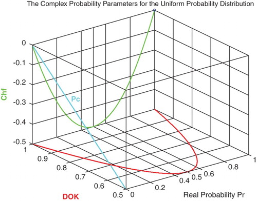
Figure 2. DOK, Chf, and P_c for the uniform probability distribution with .

What is interesting here is thus we have quantified both the DOK and the chaotic factor of any random event and hence we write now (5) Then we can conclude that therefore .

This directly means that if we succeed to subtract and eliminate the chaotic factor in any random experiment, then the output will always be with the probability equal to 1 (Dacunha-Castelle, 1996; Dalmedico-Dahan, Chabert, & Chemla, 1992; Dalmedico-Dahan & Peiffer, 1986; Ekeland, 1991; Gleick, 1997; Gullberg, 1997; Science Et Vie, 1999).

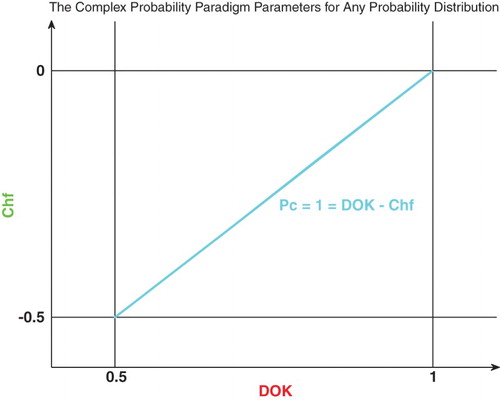
Figure 3 shows the linear relation between both DOK and Chf.

Figure 3. Graph of .

Furthermore, we need in our current study the absolute value of the chaotic factor that will give us the magnitude of the chaotic and random effects on the studied system materialized by the probability density function (PDF), and which leads to an increasing system chaos in . This new term will be denoted accordingly MChf or magnitude of the chaotic factor (Figures 4–6). Hence, we can deduce the following results: (6) and , where .

Figure 4. Graph of .

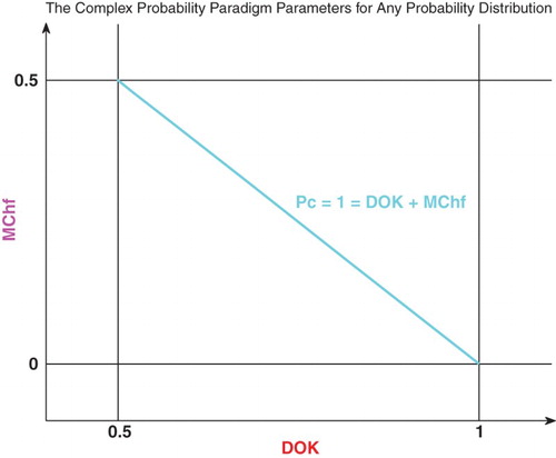
Figure 5. MChf, DOK, and P_C for the uniform probability distribution with .

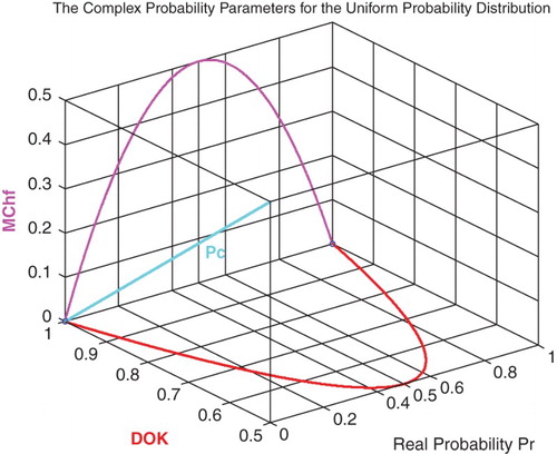
Figure 6. Chf and MChf for the uniform probability distribution with MChf + Chf = 0.

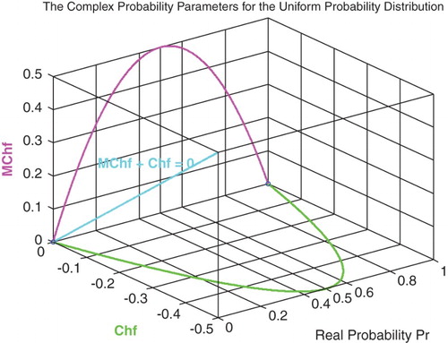
Figure 4 shows the linear relation between both DOK and MChf. Moreover, Figures 5 and 6 show the graphs of Chf, MChf, DOK, and P_c as functions of the real probability P_r for a uniform probability distribution.

To summarize and to conclude, as the Degree of Our certain Knowledge or DOK in the real universe is unfortunately incomplete, the extension to the complex set includes the contributions of both the real set of probabilities and the imaginary set of probabilities . Consequently, this will result in a complete and perfect degree of knowledge in  =  +  (P_C = 1). 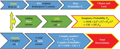In fact, in order to have a certain prediction of any random event, it is necessary to work in the complex set in which the chaotic factor is quantified and subtracted from the computed degree of knowledge to lead to a probability in equal to one (P_c² = DOK − Chf = DOK + MChf = 1). This hypothesis is verified in my six previous research papers by the mean of many examples encompassing both discrete and continuous distributions (Abou Jaoude, 2013a, 2013b, 2014, 2015a, 2015b; Abou Jaoude et al., 2010). The extended Kolmogorov axioms (EKA for short) or the CPP can be illustrated by Figure 7.

Figure 7. The EKA or the complex probability paradigm (CPP) diagram.

5. The new paradigm and Chebyshev’s inequality (Abou Jaoude, 2004, 2005, 2007; Chan Man Fong, De Kee, & Kaloni, 1997; Stepić & Ognjanović, 2014)

The real probability in the CPP applied to Chebyshev's inequality is Let , where we have .

Therefore we can write using Chebyshev's inequality: We have from the ; so we can deduce from inequality (2) that

5.1. The DOK

We have from the ; so we can deduce from inequalities (2) and (3) that: Or Note that we have from the CPP always: .

Note that when then inequalities (4) and (5) give:

, which is logical since the real probability is Hence, we have in this case a certain event and consequently the DOK is perfect and is equal to 1 or 100%.

From inequalities (4) and (5), we can find the Midpoint of DOK denoted by MP_DOK, which is equal to (Figures 8 and 9): (7) Note that: , then

Figure 8. The midpoint of DOK function of β.

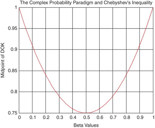
Figure 9. The midpoint of DOK function of k.

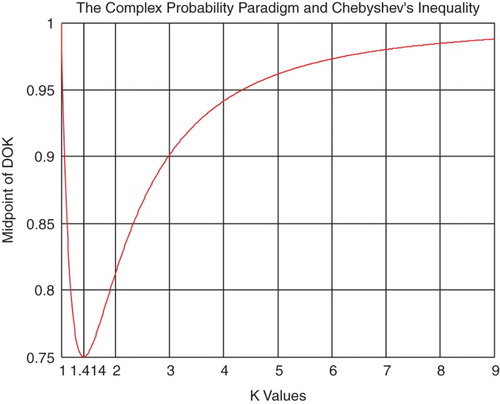
from inequality (1).

At this last point . We have , hence, MP_DOK is a curve concave upward everywhere and its minimum occurs at (0.5, 0.75). This result is very logical since we have from the CPP always: Note that

If

If from inequality (1)

or for from inequality (1)

5.2. The chaotic factor Chf

We have from the CPP Then we can deduce from inequality (2) that Therefore or Note that we have from the CPP always: .

Note that when then inequalities (6) and (7) give

, which is logical since the real probability is Hence, we have in this case a certain event and consequently the chaotic factor is null and is equal to 0.

From inequalities (6) and (7), we can find the Midpoint of Chf denoted by MP_Chf (Figures 10 and 11), which is equal to (8)

Figure 10. The midpoint of Chf function of β.

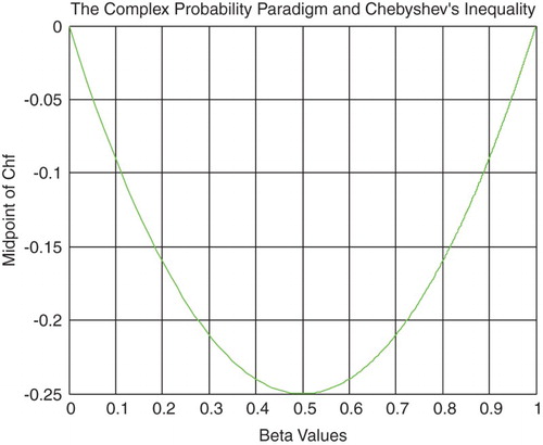
Figure 11. The midpoint of Chf function of k.

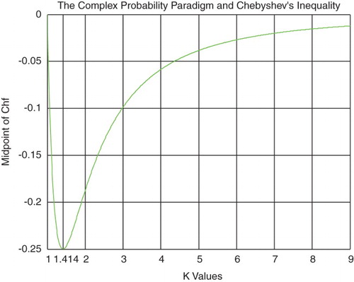
Note that , then

from inequality (1).

At this last point . We have ; hence, the MP_Chf is a curve concave upward everywhere and its minimum occurs at (0.5, −0.25). This result is very logical since we have from the CPP always Note that

If then:

for

or for

5.3. The magnitude of the chaotic factor MChf

We have from the CPP Then we can deduce from inequality (2) that Therefore, or Note that we have from the CPP always: .

Note that when then inequalities (8) and (9) give:

, which is logical since the real probability is Hence, we have in this case a certain event and consequently the magnitude of the chaotic factor is null and is equal to 0.

From inequalities (8) and (9), we can find the Midpoint of MChf denoted by , which is equal to (Figures 12 and 13) (9) Note that , then

Figure 12. The midpoint of MChf function of β.

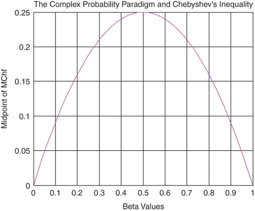
Figure 13. The midpoint of MChf function of k.

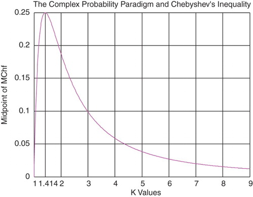
from inequality (1).

At this last point . We have ; hence, is a curve concave downward everywhere and its maximum occurs at (0.5, 0.25). This result is very logical since we have from the CPP always Note that

If then:

for from inequality (1)

or for from inequality (1).

5.4. The complex probability P_c

We have from the CPP

and we have and Therefore and Since we have from the CPP: and since we have Therefore, we get the same inequality as inequality (10) just as expected Note that we have from the CPP always: In fact, from inequalities (10) and (11), we can find the Midpoint of P_c² and P_c denoted by and , respectively, which are equal to (Figures 14 and 15) (10) and All the four figures that follow illustrate the relation between the CPP and Chebyshev's inequality (Figures 16–19).

Figure 16 shows the graphs of the midpoints of the CPP parameters in Chebyshev's inequality with the exact , and , having all of them as functions of , with .

Figure 14. The midpoint of P_c function of β.

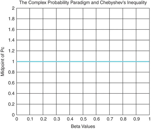
Figure 15. The midpoint of P_c function of k.

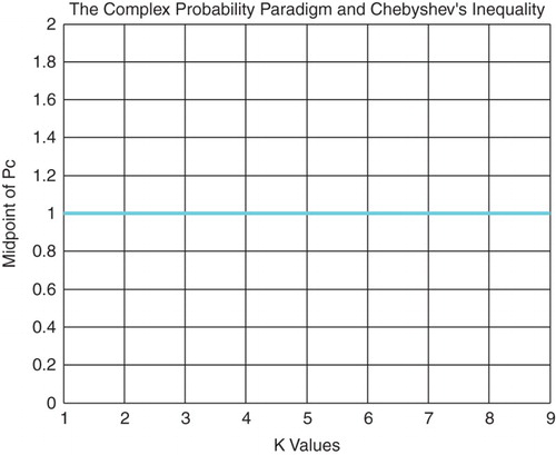
Figure 16. The midpoints of the CPP parameters functions of k.

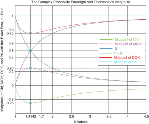
Figure 17. The midpoints and the exact CPP parameters functions of k.

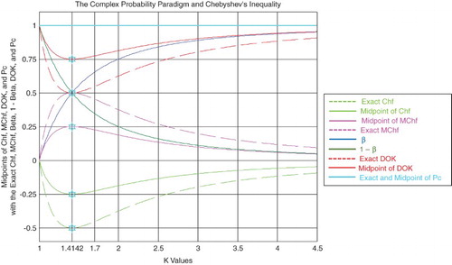
Figure 18. The midpoints of the CPP parameters functions of β.

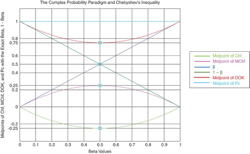
Figure 19. The midpoints and the exact CPP parameters functions of β.

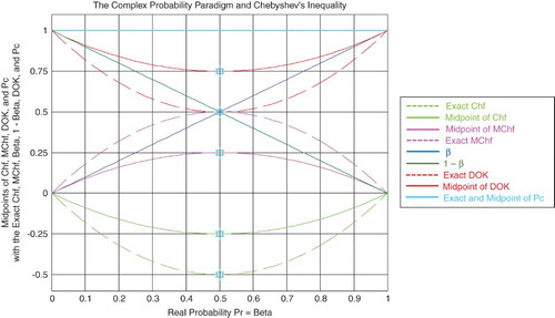
Figure 17 shows the graphs of the midpoints of the CPP parameters in Chebyshev's inequality with the exact , and , having all of them as functions of k. In addition, I have plotted on the same figure the exact CPP parameters graphs by taking the required simulation's real probability , with .

Figure 18 shows the graphs of the midpoints of the CPP parameters in Chebyshev's inequality with the exact , and , having all of them now as functions of , with .

Figure 19 shows the graphs of the midpoints of the CPP parameters in Chebyshev's inequality with the exact , and , having all of them as functions of . In addition, I have plotted on the same figure the exact CPP parameters graphs by taking the required simulation's real probability , with .

5.5. The complex random vector z

We have from the CPP the complex random vector , then inequality (2) + inequality (3) give or Then and From inequalities (12) and (13), we can find the Midpoint of the complex random vector z denoted by , which is equal to (11) Note that (Figures 20 and 21): Note that

the slope of the MP_z line in the plane whose equation is (Figure 20) (Tables 1–3).

Figure 20. The complex probability vector z midpoint and Chebyshev's inequality function of β.

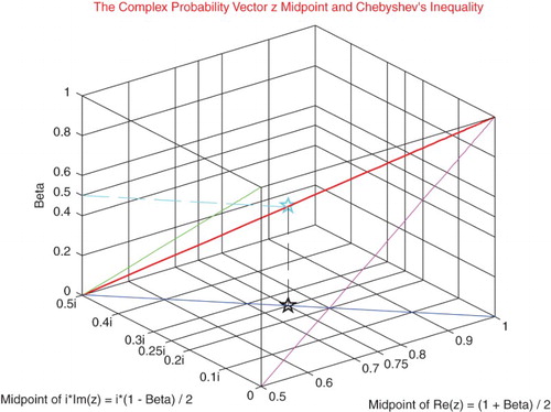
Figure 21. The complex probability vector z midpoint and Chebyshev's inequality function of k.

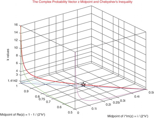
Table 1. The CPP and Chebyshev's inequality for 1 ≤ k ≤ 2.

Midpoints/k values	k = 1	k = 1.2		k = 2
	0	0.3056	0.5000	0.7500
	1	0.6944	0.5000	0.2500
MP of Pr	0.5000	0.6528	0.7500	0.8750
MP of Pm/i	0.5000	0.3472	0.2500	0.1250
MP of z	0.5000 + 0.5000i	0.6528 + 0.3472i	0.7500 + 0.2500i	0.8750 + 0.1250i
MP of DOK	1	0.7878	0.7500	0.8125
MP of Chf	0	−0.2122	−0.2500	−0.1875
MP of MChf	0	0.2122	0.2500	0.1875
MP of PC	1	1	1	1

Table 2. The CPP and Chebyshev's inequality for 3 ≤ k ≤ 100.

Midpoints/k values	k = 3	k = 5	k = 10	k = 100
	0.8889	0.9600	0.9900	0.9999
	0.1111	0.0400	0.0100	0.0001
MP of Pr	0.94445	0.9800	0.9950	0.99995
MP of Pm/i	0.05555	0.0200	0.0050	0.00005
MP of z	0.94445 + 0.05555i	0.9800 + 0.0200i	0.995 + 0.005i	0.99995 + 0.00005i
MP of DOK	0.90124321	0.9616	0.9901	0.99990001
MP of Chf	−0.09875679	−0.03840	−0.0099	−0.00009999
MP of MChf	0.09875679	0.03840	0.0099	0.00009999
MP of PC	1	1	1	1

Table 3. The CPP and Chebyshev's inequality for k = 1000 and 10,000.

Midpoints/k values	k = 1000	k = 10,000
	0.999999	0.99999999 ≈ 1
	0.000001	0.00000001 ≈ 0
MP of Pr	0.9999995	0.999999995 ≈ 1
MP of Pm/i	0.0000005	0.000000005 ≈ 0
MP of z	0.9999995 + 0.0000005i	0.999999995 + 0.000000005i ≈ 1 + 0i
MP of DOK	0.999999000001	0.9999999900000001 ≈ 1
MP of Chf	−9.99999e−7	−9.9999999e−9 ≈ 0
MP of MChf	9.99999e−7	9.9999999e−9 ≈ 0
MP of PC	1	1

6. Numerical simulations of discrete and continuous distributions and Chebyshev’s inequality (Abou Jaoude, 2013a, 2013b, 2014, 2015a, 2015b; Abou Jaoude et al., 2010; Wikipedia, Probability Theory, Probability Distribution, Probability Density Function, Probability Space, Probability Measure, Probability Axioms, Chebyshev’s Inequality, Pafnuty Chebyshev, Markov’s Inequality)

6.1. The evaluation of the CPP parameters

The cumulative distribution function (CDF) of the discrete or continuous random variable x is denoted by .

Then the CPP parameters are the following: (12) (13) (14) (15)

The DOK: (16) The chaotic factor (Chf): (17) The magnitude of the chaotic factor (MChf): (18) At any value of the random variable x, the probability expressed in the complex set is (19) Then, always; hence, the prediction of the outcome of the random variable x in is permanently certain and absolutely deterministic.

Note that all the numerical values found in the paradigm functions analysis and Chebyshev's inequality for all the values of k and β were computed using the MATLAB version 2016 software.

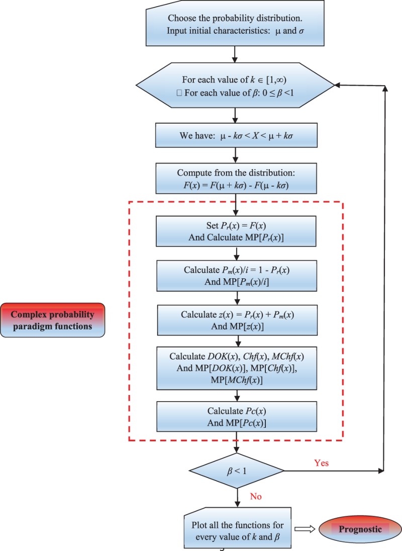
6.2. Flowchart of the CPP applied to Chebyshev’s inequality

The following flowchart summarizes all the procedures of the proposed complex probability prognostic model:

6.3. Numerical simulation of the continuous uniform probability distribution:

The PDF of this continuous distribution is (20) and the CDF is (21) I have taken the domain for the continuous uniform random variable to be: and then The real probability is The complementary probability P_m(x)/i is The other parameters are calculated from the CPP paradigm (refer to Section 6.1).

The mean of this continuous uniform random distribution is .

The standard deviation is (Figures 22 and 23) (Tables 4 and 5).

Figure 22. The CPP parameters for the continuous uniform distribution.

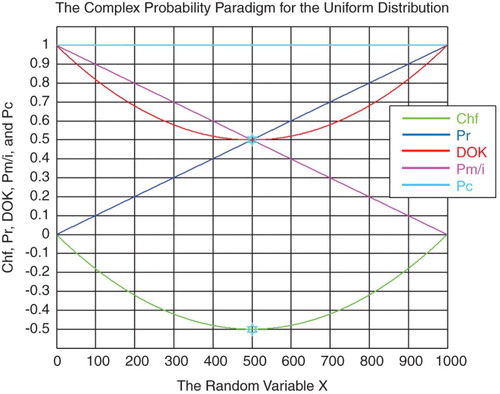
Figure 23. The CPP parameters with MChf for the continuous uniform distribution.

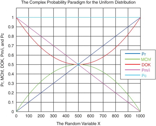
Table 4. The CPP and Chebyshev's inequality for the continuous uniform distribution for k = 1, 1.1, and 1.3.

The paradigm values	211.32 < X < 788.68	182.45 < X < 817.55	124.72 < X < 875.28
k	1.000000000	1.100000000	1.300000000
	0	0.173553719	0.408284023
	1	0.826446281	0.591715977
MP of Pr	0.500000000	0.586776859	0.704142011
Exact Pr	0.577350269	0.635085296	0.750555350
MP of Pm/i	0.500000000	0.413223141	0.295857989
Exact Pm/i	0.422649731	0.364914704	0.249444650
MP of z	0.50000 + 0.50000i	0.58678 + 0.41322i	0.70414 + 0.29586i
Exact z	0.57735 + 0.42265i	0.63509 + 0.36491i	0.75056 + 0.24944i
MP of DOK	1	0.856567175	0.758411821
Exact DOK	0.511966128	0.536496075	0.625555967
MP of Chf	0	−0.143432825	−0.241588179
Exact Chf	−0.488033872	−0.463503925	−0.374444033
MP of MChf	0	0.143432825	0.241588179
Exact MChf	0.488033872	0.463503925	0.374444033
MP of PC	1	1	1
Exact PC	1	1	1

Table 5. The CPP and Chebyshev's inequality for the continuous uniform distribution for , 1.6, and .

The paradigm values	91.75 < X < 908.25	38.12 < X < 961.89	0 < X < 1000
k		1.600000000
	0.500000000	0.609375000	0.666666667
	0.500000000	0.390625000	0.333333333
MP of Pr	0.750000000	0.804687500	0.833333333
Exact Pr	0.816496581	0.923760430	0.999999998 ≈ 1
MP of Pm/i	0.250000000	0.195312500	0.166666667
Exact Pm/i	0.183503419	0.076239570	0.000000002 ≈ 0
MP of z	0.75000 + 0.25000i	0.80469 + 0.19531i	0.83333 + 0.16667i
Exact z	0.81650 + 0.18350i	0.92376 + 0.07624i	≈1 + 0i
MP of DOK	0.750000000	0.761962891	0.777777778
Exact DOK	0.700340171	0.859145805	0.999999996 ≈ 1
MP of Chf	−0.250000000	−0.238037109	−0.222222222
Exact Chf	−0.299659829	−0.140854195	−3.999999968e−9 ≈ 0
MP of MChf	0.250000000	0.238037109	0.222222222
Exact MChf	0.299659829	0.140854195	3.999999968e−9 ≈ 0
MP of PC	1	1	1
Exact PC	1	1	1

6.4. Numerical simulation of the binomial probability distribution

The PDF of this discrete distribution is (22) and the CDF is (23) I have taken the domain for the binomial random variable to be: and , then: .

The real probability is The complementary probability P_m(x)/i is The other parameters are calculated from the CPP paradigm (refer to Section 6.1).

Taking in our simulation and , then the mean of this binomial random distribution is , and the standard deviation is (Figures 24 and 25) (Tables 6 and 7).

Figure 24. The CPP parameters for the binomial distribution.

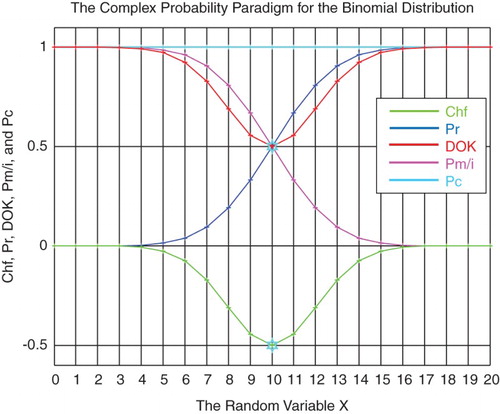
Figure 25. The CPP parameters with MChf for the binomial distribution.

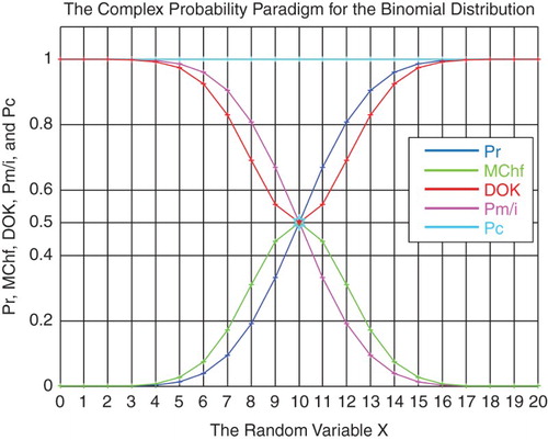
Table 6. The CPP and Chebyshev's inequality for the binomial distribution for k = 1.34, 1.79, and 2.24.

The paradigm values	7 < X < 13	6 < X < 14	5 < X < 15
k	1.341640787	1.788854382	2.236067978
	0.444444444	0.687500000	0.800000000
	0.555555556	0.312500000	0.200000000
MP of Pr	0.722222222	0.843750000	0.900000000
Exact Pr	0.713680000	0.866220000	0.947500000
MP of Pm/i	0.277777778	0.156250000	0.100000000
Exact Pm/i	0.286320000	0.133780000	0.052500000
MP of z	0.72222 + 0.27778i	0.84375 + 0.15625i	0.90000 + 0.10000i
Exact z	0.71368 + 0.28632i	0.86622 + 0.13378i	0.94750 + 0.05250i
MP of DOK	0.753086419	0.785156250	0.840000000
Exact DOK	0.591318284	0.768234177	0.900512500
MP of Chf	−0.246913581	−0.214843750	−0.160000000
Exact Chf	−0.408681716	−0.231765823	−0.099487500
MP of MChf	0.246913581	0.214843750	0.160000000
Exact MChf	0.408681716	0.231765823	0.099487500
MP of PC	1	1	1
Exact PC	1	1	1

Table 7. The CPP and Chebyshev's inequality for the binomial distribution for k = 2.68, 3.58, and 4.47.

The paradigm values	4 < X < 16	2 < X < 18	0 < X < 20
k	2.683281573	3.577708764	4.472135955
	0.861111111	0.921875000	0.950000000
	0.138888889	0.078125000	0.050000000
MP of Pr	0.930555556	0.960937500	0.975000000
Exact Pr	0.983101000	0.999189400	0.999998092
MP of Pm/i	0.069444444	0.039062500	0.025000000
Exact Pm/i	0.016899000	0.000810600	0.000001908
MP of z	0.93056 + 0.06944i	0.96094 + 0.03906i	0.97500 + 0.02500i
Exact z	0.98310 + 0.01690i	0.99919 + 0.00081i	0.9999981 + 1.9e−6i
MP of DOK	0.880401235	0.927978515	0.952500000
Exact DOK	0.966773153	0.998380114	0.999996184
MP of Chf	−0.119598765	−0.072021485	−0.047500000
Exact Chf	−0.033226847	−0.001619886	−3.815992719e−6
MP of MChf	0.119598765	0.072021485	0.047500000
Exact MChf	0.033226847	0.001619886	3.815992719e−6
MP of PC	1	1	1
Exact PC	1	1	1

6.5. Numerical simulation of the Poisson probability distribution

The PDF of this discrete distribution is (24) and the CDF is (25) For the Poisson random variable: and , then .

The real probability is The complementary probability P_m(x)/i is The other parameters are calculated from the CPP paradigm (refer to Section 6.1).

Taking in our simulation , then the mean of this Poisson random distribution is , and the standard deviation is (Figures 26 and 27) (Tables 8 and 9).

Figure 26. The CPP parameters for the Poisson distribution.

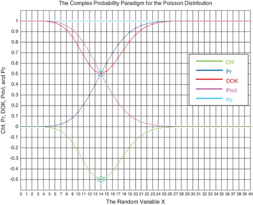
Figure 27. The CPP parameters with MChf for the Poisson distribution.

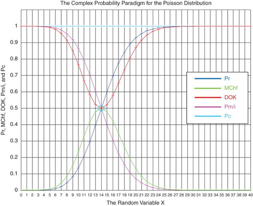
Table 8. The CPP and Chebyshev's inequality for the Poisson distribution for k = 1.22, 1.74, and 2.26.

The paradigm values	10 < X < 19.336	8 < X < 21.336	6 < X < 23.336
k	1.218836347	1.741045578	2.263254810
	0.326854097	0.670101972	0.804776049
	0.673145903	0.329898028	0.195223951
MP of Pr	0.663427049	0.835050986	0.902388025
Exact Pr	0.757400000	0.911780000	0.975191000
MP of Pm/i	0.336572951	0.164949014	0.097611975
Exact Pm/i	0.242600000	0.088220000	0.024809000
MP of z	0.66343 + 0.33657i	0.83505 + 0.16495i	0.90239 + 0.09761i
Exact z	0.75740 + 0.24260i	0.91178 + 0.08822i	0.97519 + 0.02481i
MP of DOK	0.779979504	0.778934681	0.842888440
Exact DOK	0.632509520	0.839125537	0.951612973
MP of Chf	−0.220020496	−0.221065319	−0.157111560
Exact Chf	−0.367490480	−0.160874463	−0.048387027
MP of MChf	0.220020496	0.221065319	0.157111560
Exact MChf	0.367490480	0.160874463	0.048387027
MP of PC	1	1	1
Exact PC	1	1	1

Table 9. The CPP and Chebyshev's inequality for the Poisson distribution for k = 2.79, 3.31, and 3.83.

The paradigm values	4 < X < 25.336	2 < X < 27.336	0 < X < 29.336
k	2.785464041	3.307673273	3.829882505
	0.871114254	0.908598190	0.931824379
	0.128885746	0.091401810	0.068175621
MP of Pr	0.935557127	0.954299095	0.965912189
Exact Pr	0.994201000	0.998647460	0.999699573
MP of Pm/i	0.064442873	0.045700905	0.034087811
Exact Pm/i	0.005799000	0.001352540	0.000300427
MP of z	0.93556 + 0.06444i	0.95430 + 0.04570i	0.96591 + 0.03409i
Exact z	0.99420 + 0.00580i	0.99865 + 0.00135i	0.99970 + 0.00030i
MP of DOK	0.887725789	0.916952481	0.936472294
Exact DOK	0.988469256	0.997298579	0.999399327
MP of Chf	−0.112274211	−0.083047519	−0.063527706
Exact Chf	−0.011530744	−0.002701421	−0.000600673
MP of MChf	0.112274211	0.083047519	0.063527706
Exact MChf	0.011530744	0.002701421	0.000600673
MP of PC	1	1	1
Exact PC	1	1	1

6.6. Numerical simulation of the normal Gauss–Laplace probability distribution:

The PDF of this continuous distribution is (26) and the CDF is (27) The domain for this normal variable is and I have taken .

The real probability is The complementary probability P_m(x)/i is The other parameters are calculated from the CPP paradigm (refer to Section 6.1).

In the simulation, I have taken the mean of this normal random distribution to be: ,

and the standard deviation is (Figures 28 and 29) (Tables 10–12).

Figure 28. The CPP parameters for the normal distribution.

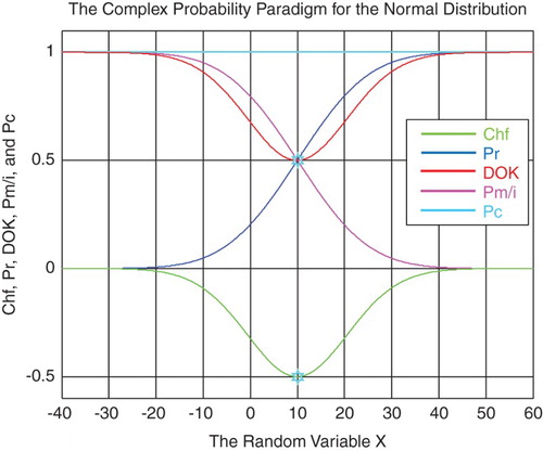
Figure 29. The CPP parameters with MChf for the normal distribution.

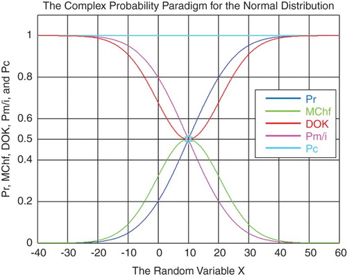
Table 10. The CPP and Chebyshev's inequality for the normal distribution for k = 1, 1.01, and 1.1.

The paradigm values	−2 < X < 22	−2.12 < X < 22.12	−3.2 < X < 23.2
k	1.000000000	1.010000000	1.100000000
	0	0.019703950	0.173553719
	1	0.980296050	0.826446281
MP of Pr	0.500000000	0.509851975	0.586776859
Exact Pr	0.682500000	0.687300000	0.728500000
MP of Pm/i	0.500000000	0.490148025	0.413223141
Exact Pm/i	0.317500000	0.312700000	0.271500000
MP of z	0.50000 + 0.50000i	0.50985 + 0.49015i	0.58678 + 0.41322i
Exact z	0.68250 + 0.31750i	0.68730 + 0.31270i	0.72850 + 0.27150i
MP of DOK	1	0.980684296	0.856567175
Exact DOK	0.566612500	0.570162580	0.604424500
MP of Chf	0	−0.019315704	−0.143432825
Exact Chf	−0.433387500	−0.429837420	−0.395575500
MP of MChf	0	0.019315704	0.143432825
Exact MChf	0.433387500	0.429837420	0.395575500
MP of PC	1	1	1
Exact PC	1	1	1

Table 11. The CPP and Chebyshev's inequality for the normal distribution for k = 1.25, 1.5, and 2.

The paradigm values	−5 < X < 25	−8 < X < 28	−14 < X < 34
k	1.250000000	1.500000000	2.000000000
	0.360000000	0.555555556	0.750000000
	0.640000000	0.444444444	0.250000000
MP of Pr	0.680000000	0.777777778	0.875000000
Exact Pr	0.788600000	0.866280000	0.954420000
MP of Pm/i	0.320000000	0.222222222	0.125000000
Exact Pm/i	0.211400000	0.133720000	0.045580000
MP of z	0.68000 + 0.32000i	0.77778 + 0.22222i	0.87500 + 0.12500i
Exact z	0.78860 + 0.21140i	0.86628 + 0.13372i	0.95442 + 0.04558i
MP of DOK	0.769600000	0.753086419	0.812500000
Exact DOK	0.666579920	0.768322076	0.912995072
MP of Chf	−0.230400000	−0.246913581	−0.187500000
Exact Chf	−0.333420080	−0.231677924	−0.087004928
MP of MChf	0.230400000	0.246913581	0.187500000
Exact MChf	0.333420080	0.231677924	0.087004928
MP of PC	1	1	1
Exact PC	1	1	1

Table 12. The CPP and Chebyshev's inequality for the normal distribution for k = 2.75, 3.5, and 10.

The paradigm values	−23 < X < 43	−32 < X < 52	−110 < X < 130
k	2.750000000	3.500000000	10.000000000
	0.867768595	0.918367346	0.990000000
	0.132231405	0.081632654	0.010000000
MP of Pr	0.933884297	0.959183673	0.995000000
Exact Pr	0.994016000	0.999567000	≈ 1
MP of Pm/i	0.066115703	0.040816327	0.005000000
Exact Pm/i	0.005984000	0.000433000	≈ 0
MP of z	0.93388 + 0.06612i	0.95918 + 0.04082i	0.99500 + 0.00500i
Exact z	0.99402 + 0.00598i	0.99957 + 0.00043i	≈ 1 + 0i
MP of DOK	0.885253739	0.925031237	0.990100000
Exact DOK	0.988103616	0.999134375	≈ 1
MP of Chf	−0.114746261	−0.074968763	−0.009900000
Exact Chf	−0.011896384	−0.000865625	≈ 0
MP of MChf	0.114746261	0.074968763	0.009900000
Exact MChf	0.011896384	0.000865625	≈ 0
MP of PC	1	1	1
Exact PC	1	1	1

7. The resultant complex random vector Z and Chebyshev’s inequality (Bidabad, 1992; Cox, 1955; Fagin, Halpern, & Megiddo, 1990; Ognjanović, Marković, Rašković, Doder, & Perović, 2012; Weingarten, 2002; Youssef, 1994)

7.1. The resultant complex random vector Z

As a general case, let us consider then this discrete probability distribution with N disjoint and independent random variables (Table 13):

Table 13. The discrete probability distribution with N random variables.

Random variables
Probabilities in
Probabilities in

We can see that We have here in  =  +  the complex random vector corresponding to each random variable for : and the corresponding vector norm of is In addition, we have The resultant complex random vector Z representing the whole random distribution is (28)

Then we can deduce the following results: the mean of the real probabilities of all the complex random vectors and the mean of the imaginary probabilities of all the complex random vectors ; hence, .

Note that we have for the random vector , which is the mean of the resultant complex random vector Z: , just like for all the complex random vectors .

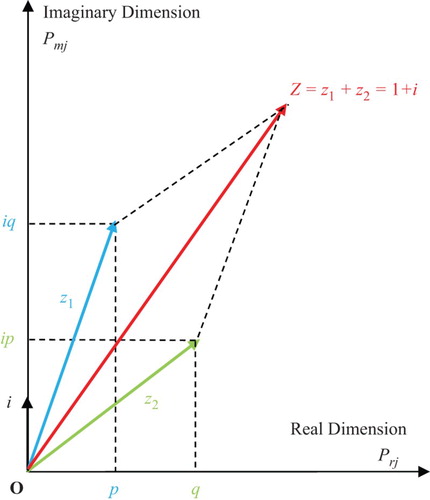
Moreover, we can note that the norm of Z can be computed in the following way: Having (29) Or we can calculate the norm of Z in a different way using To illustrate the concept of the resultant complex random vector Z, I will use Figure 30.

Figure 30. The resultant complex random vector for a general distribution with N = 2 (Bernoulli distribution) in the complex probability plane .

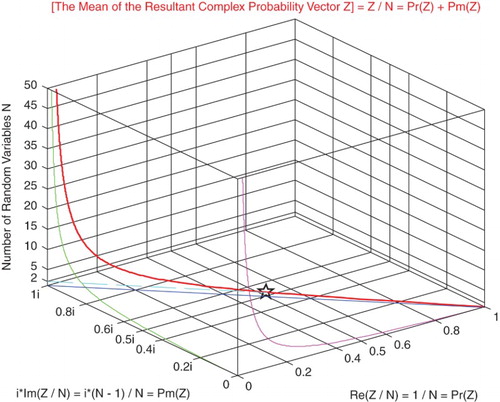
Moreover, to clarify the concept of the resultant complex random vector Z related to Chebyshev's inequality, I will present Figure 31.

Figure 31. The mean of the resultant complex vector which is Z/N function of the number of random variables N.

7.2. The knowledge and the chaos related to Z

For any complex random vector we have for :

And .

For the resultant complex random vector we have (30) (31) (32) (33)

And .

Therefore, the DOK corresponding to the resultant complex vector Z representing the whole distribution of random variables is (34) and its relative chaotic factor is (35) Similarly, its relative magnitude of the chaotic factor is (36) Thus we can verify that we have always We can deduce mathematically that (37) (38) (39) From the above, we can also deduce this conclusion:

As much as N increases, as much as the DOK in corresponding to the resultant complex vector is perfect, that is, it is equal to 1, and as much as the chaotic factor that forbids us from predicting exactly the result of the random experiment in approaches 0. Mathematically we say: If N tends to infinity then the DOK in tends to 1 and the chaotic factor tends to 0.

Moreover, This means that for we have a random experiment with only one outcome, hence, either or , which means we have, respectively, either a sure event or an impossible event in . For this we have surely the DOK is 1 and the chaotic factor is 0 since the experiment is either certain or impossible, which is absolutely logical.

It is important to note that if in addition the outcomes of the random variables are equiprobable, then we get Table 14:

Table 14. The discrete probability distribution with N equiprobable random variables.

Random variables
Probabilities in
Probabilities in

Then, Therefore and for .

Hence And Consequently, these results follow: (40) (41) and (42) Therefore (43)

7.3. Applying Chebyshev’s Inequality to Z

For a probability distribution of N disjoint and independent random variables, we have:

Since then

since

then

and since

Then .

So we can deduce the following results (Figures 32–35): (44)

Figure 32. |Z|² with the lower and upper bounds functions of N and k.

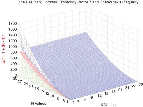
Figure 33. The midpoint of DOK(Z) function of N and k.

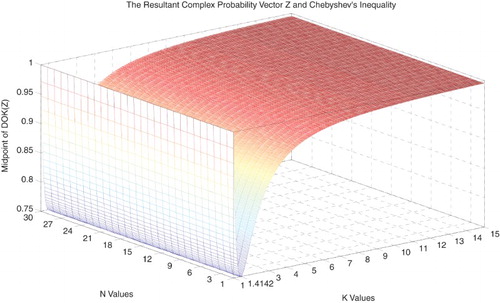
Figure 34. The midpoint of DOK(Z) with the lower and upper bounds functions of N and k.

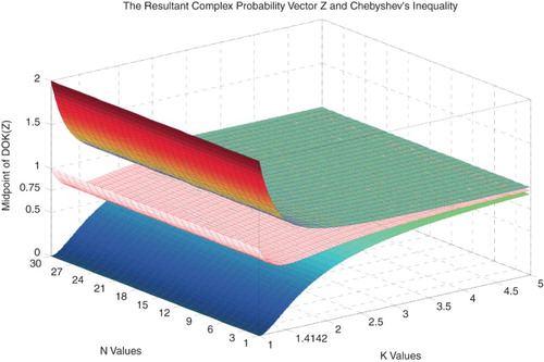
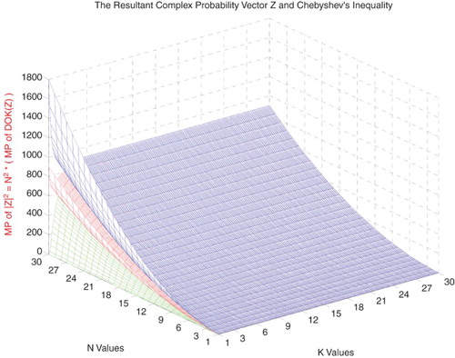
Figure 35. The midpoint of |Z|² with the lower and upper bounds functions of N and k.

Now since

Then , and

Furthermore, since

Then, and

Therefore, and since then, Thus, we have reached the same inequality for in a different way.

Figure 36. N² × Chf(Z) with the lower and upper bounds functions of N and k.

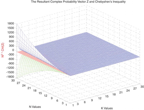
Figure 37. The midpoint of Chf(Z) function of N and k.

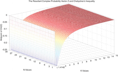
Figure 38. The midpoint of Chf(Z) with the lower and upper bounds functions of N and k.

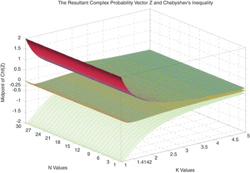
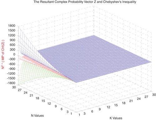
Figure 39. N² × midpoint of Chf(Z) with the lower and upper bounds functions of N and k.

Additionally we can deduce that (Figures 36–39): and

So it follows that: (45)

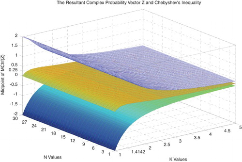
Moreover,

Since .

Then (Figures 40 and 41) (46)

Figure 40. The midpoint of MChf(Z) function of N and k.

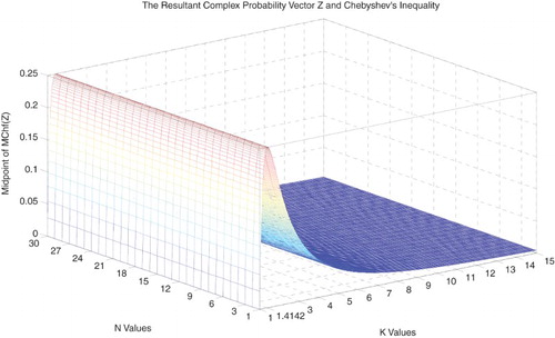
Figure 41. The midpoint of MChf(Z) with the lower and upper bounds functions of N and k.

In addition, we have from the CPP: Therefore, And since we have from the CPP: , therefore, we get the same inequality just as expected: Note that we have from the CPP always: Consequently, we can find the Midpoint of and denoted by and , respectively, and which are equal to: (47)

and And ; .

8. The complex characteristics of the probability distributions (Abou Jaoude, 2013a, 2013b, 2014, 2015a, 2015b; Abou Jaoude et al., 2010; Benton, 1966a, 1966b; Feller, 1968; Montgomery & Runger, 2003; Walpole et al., 2002)

8.1. The expectation in

8.1.1. The general probability distribution case

As a general case, let us consider then this discrete probability distribution with N random variables (Table 13):

We can see that

And similarly, we have

We have also (48) Moreover,

Furthermore, and Then,

The conjugate of Z is And let .

Now, we define the conjugate of by Therefore, we get the following relations: And .

And since and

8.1.2. The general Bernoulli distribution case

Let us consider then this general Bernoulli discrete probability distribution with N = 2 random variables (Table 15):

Table 15. The general Bernoulli distribution with N = 2.

Random outcomes
Probabilities in
Probabilities in

We can see that

With and Additionally, And similarly, we have We have also

Moreover, With , Furthermore, And the conjugate of Z is

Then and

And let

We can deduce mathematically that for any Bernoulli distribution we have that (49) (50) (51) (52) (53) (54) (55) (56)

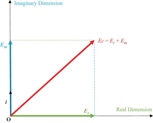
To illustrate the concept of complex expectation, I will use Figure 42.

8.2. The variance in

As a general case, let us consider then the discrete probability distribution with N random variables (Table 13).

Figure 42. The complex expectation Ec = E_r + E_m in the complex probability plane .

The expectation of the real part of the random variables is defined by The expectation of the imaginary part of the random variables is defined by The expectation of the complex random variables is defined by We have also:

The variance of the real part of the random variables is defined by: (57) The variance of the imaginary part of the random variables is defined by: (58) The variance of the complex random variables is defined by: (59) But ,

Thus (60)

8.3. A numerical example of a Bernoulli distribution

Let us consider the following Bernoulli discrete probability distribution with N = 2 random outcomes (Table 16):

Table 16. An example of a Bernoulli distribution with N = 2.

Random outcomes
Probabilities in
Probabilities in

We can see that

And similarly, we have We have also Moreover

The conjugate of Z is

Then and

And let . We can verify easily the following relations:

And we can verify that And we have: , just as expected and proved.

8.4. Numerical simulations (Gentle, 2003)

Numerical simulations verify what has been found earlier. I will use Monte Carlo simulation method with the help of the programming language C++ with its predefined pseudorandom function rand() to generate random numbers with a uniform distribution. To summarize what the seven tables that follow describe:

• Tables 17–19, are simulations of a Bernoulli distribution where the complex random vectors are chosen randomly by C++.

• Tables 20–23 are simulations of a uniform distribution with three random variables having their complex random vectors also chosen randomly by C++.

Table 17. Computation of for different of values of and which are the complex random vectors of a Bernoulli distribution and which are chosen at random.

The complex random vectors and their probabilities
Simulation #1	0.8106 + i(0.1894)	1	0.1894 + i(0.8106)	1	1 + i	1
Simulation #2	0.0084 + i(0.9916)	1	0.9916 + i(0.0084)	1	1 + i	1
Simulation #3	0.4558 + i(0.5442)	1	0.5442 + i(0.4558)	1	1 + i	1
Simulation #4	0.5225 + i(0.4775)	1	0.4775 + i(0.5225)	1	1 + i	1
Simulation #5	0.3723 + i(0.6277)	1	0.6277 + i(0.3723)	1	1 + i	1
Simulation #6	0.1908 + i(0.8092)	1	0.8092 + i(0.1908)	1	1 + i	1
Simulation #7	0.208 + i(0.792)	1	0.792 + i(0.208)	1	1 + i	1

Note: In this case, the resultant complex random vector is and is always equal to with always.

Table 18. Computation of the real, imaginary and complex expectations for different of values of and , which are chosen at random and the verification that we have always .

The complex random vectors and their characteristics
Simulation #1	0.8106 + i(0.1894)	0.1894 + i(0.8106)	1 + i	1.189	i(1.811)	1.189 + i(1.811)
Simulation #2	0.0084 + i(0.9916)	0.9916 + i(0.0084)	1 + i	1.992	i(1.008)	1.992 + i(1.008)
Simulation #3	0.4558 + i(0.5442)	0.5442 + i(0.4558)	1 + i	1.544	i(1.456)	1.544 + i(1.456)
Simulation #4	0.5225 + i(0.4775)	0.4775 + i(0.5225)	1 + i	1.478	i(1.522)	1.478 + i(1.522)
Simulation #5	0.3723 + i(0.6277)	0.6277 + i(0.3723)	1 + i	1.628	i(1.372)	1.628 + i(1.372)
Simulation #6	0.1908 + i(0.8092)	0.8092 + i(0.1908)	1 + i	1.809	i(1.191)	1.809 + i(1.191)
Simulation #7	0.208 + i(0.792)	0.792 + i(0.208)	1 + i	1.792	i(1.208)	1.792 + i(1.208)

Table 19. Computation of the real, imaginary and complex variances for different of values of and , which are chosen at random and the verification that we have always .

The complex random vectors and their characteristics
Simulation #1	0.8106 + i(0.1894)	0.1894 + i(0.8106)	1 + i	0.1535	3.278 + i(3.432)	3.432 + i(−0.8753)
Simulation #2	0.0084 + i(0.9916)	0.9916 + i(0.0084)	1 + i	0.008292	1.017 + i(1.025)	1.025 + i(−2.991)
Simulation #3	0.4558 + i(0.5442)	0.5442 + i(0.4558)	1 + i	0.248	2.119 + i(2.367)	2.367 + i(−2.129)
Simulation #4	0.5225 + i(0.4775)	0.4775 + i(0.5225)	1 + i	0.2495	2.318 + i(2.567)	2.567 + i(−1.931)
Simulation #5	0.3723 + i(0.6277)	0.6277 + i(0.3723)	1 + i	0.2337	1.883 + i(2.117)	2.117 + i(−2.35)
Simulation #6	0.1908 + i(0.8092)	0.8092 + i(0.1908)	1 + i	0.1544	1.418 + i(1.572)	1.572 + i(−2.736)
Simulation #7	0.208 + i(0.792)	0.792 + i(0.208)	1 + i	0.1647	1.459 + i(1.624)	1.624 + i(−2.705)

Table 20. Computation of for different of values of , , , which are the complex random vectors of the distribution and which are chosen at random.

The complex random vectors and their probabilities
Simulation #1	0.636 + i(0.364)	1	0.136 + i(0.864)	1	0.228 + i(0.772)	1	1 + i(2)	1
Simulation #2	0.8393 + i(0.1607)	1	0.0402 + i(0.9598)	1	0.1205 + i(0.8795)	1	1 + i(2)	1
Simulation #3	0.7802 + i(0.2198)	1	0.0220 + i(0.978)	1	0.1978 + i(0.8022)	1	1 + i(2)	1
Simulation #4	0.3619 + i(0.6381)	1	0.1381 + i(0.8619)	1	0.5 + i(0.5)	1	1 + i(2)	1
Simulation #5	0.9909 + i(0.0091)	1	0.0015 + i(0.9985)	1	0.0076 + i(0.9924)	1	1 + i(2)	1
Simulation #6	0.5205 + i(0.4795)	1	0.0533 + i(0.9467)	1	0.4262 + i(0.5738)	1	1 + i(2)	1
Simulation #7	0.0651 + i(0.9349)	1	0.2349 + i(0.7651)	1	0.7 + i(0.3)	1	1 + i(2)	1

Note: In this case, the resultant complex random vector is and is always equal to with always.

Table 21. Computation of the real, imaginary and complex expectations for different of values of , , , which are chosen at random and the verification that we have always .

The complex random vectors and their characteristics
Simulation #1	0.636 + i(0.364)	0.136 + i(0.864)	0.228 + i(0.772)	1.592	i(4.408)	1.592 + i(4.408)
Simulation #2	0.8393 + i(0.1607)	0.0402 + i(0.9598)	0.1205 + i(0.8795)	1.281	i(4.719)	1.281 + i(4.719)
Simulation #3	0.7802 + i(0.2198)	0.0220 + i(0.978)	0.1978 + i(0.8022)	1.418	i(4.582)	1.418 + i(4.582)
Simulation #4	0.3619 + i(0.6381)	0.1381 + i(0.8619)	0.5 + i(0.5)	2.138	i(3.862)	2.138 + i(3.862)
Simulation #5	0.9909 + i(0.0091)	0.0015 + i(0.9985)	0.0076 + i(0.9924)	1.017	i(4.983)	1.017 + i(4.983)
Simulation #6	0.5205 + i(0.4795)	0.0533 + i(0.9467)	0.4262 + i(0.5738)	1.906	i(4.094)	1.906 + i(4.094)
Simulation #7	0.0651 + i(0.9349)	0.2349 + i(0.7651)	0.7 + i(0.3)	2.635	i(3.365)	2.635 + i(3.365)

Table 22. Computation of the real, imaginary and complex variances for different of values of , , , which are chosen at random and the verification that we have always .

The complex random vectors and their characteristics
Simulation #1	0.636 + i(0.364)	0.136 + i(0.864)	0.228 + i(0.772)	0.6975	19.43 + i(10.77)	20.13 + i(−3.267)
Simulation #2	0.8393 + i(0.1607)	0.0402 + i(0.9598)	0.1205 + i(0.8795)	0.4431	22.27 + i(11.92)	22.71 + i(−0.1761)
Simulation #3	0.7802 + i(0.2198)	0.0220 + i(0.978)	0.1978 + i(0.8022)	0.6388	21 + i(11.35)	21.64 + i(−1.64)
Simulation #4	0.3619 + i(0.6381)	0.1381 + i(0.8619)	0.5 + i(0.5)	0.8428	14.91 + i(8.586)	15.76 + i(−7.929)
Simulation #5	0.9909 + i(0.0091)	0.0015 + i(0.9985)	0.0076 + i(0.9924)	0.03162	24.83 + i(12.93)	24.86 + i(2.802)
Simulation #6	0.5205 + i(0.4795)	0.0533 + i(0.9467)	0.4262 + i(0.5738)	0.9378	16.76 + i(9.431)	17.7 + i(−6.175)
Simulation #7	0.0651 + i(0.9349)	0.2349 + i(0.7651)	0.7 + i(0.3)	0.362	11.32 + i(6.695)	11.69 + i(−11.04)

Table 23. Computation of the real, imaginary and complex expectations and variances for different of values of , , , which are chosen at random and the verification that we have always and .

The complex random vectors and their characteristics
Simulation #1	2.635	0.362	i(3.365)	11.32 + i(6.695)	2.635 + i(3.365)	11.69 + i(−11.04)
Simulation #2	1.667	0.5556	i(4.333)	18.78 + i(10.67)	1.667 + i(4.333)	19.33 + i(−3.778)
Simulation #3	1.835	0.9288	i(4.165)	17.35 + i(9.705)	1.835 + i(4.165)	18.28 + i(−5.58)
Simulation #4	1.797	0.9167	i(4.203)	17.67 + i(9.856)	1.797 + i(4.203)	18.59 + i(−5.248)
Simulation #5	1.332	0.4876	i(4.668)	21.79 + i(11.74)	1.332 + i(4.668)	22.28 + i(−0.699)
Simulation #6	1.312	0.4817	i(4.688)	21.98 + i(11.8)	1.312 + i(4.688)	22.46 + i(−0.5012)
Simulation #7	2.428	0.7882	i(3.572)	12.76 + i(7.315)	2.428 + i(3.572)	13.54 + i(−10.03)

They are all in fact numerical simulations that confirm and quantify the results of the concepts of complex probability, expectation and variance that were determined previously.

9. Conclusion and perspectives

In the current paper I applied the Paradigm of Complex Probability to Chebyshev's inequality. Hence, I established a tight link between the new paradigm and this classical probability theorem. Thus, I developed the theory of ‘Complex Probability’ beyond the scope of my previous six papers on this topic.

I applied in this research work the pioneering model related to Chebyshev's theorem to different probability distributions which are: the uniform, the binomial, the Poisson and the normal Gauss–Laplace distributions. Moreover, as it was proved and illustrated in this work, when the CDF tends to 0 or 1 and correspondingly the real probability P_r → 0 or P_r → 1 then the DOK tends to one and the chaotic factor (Chf and MChf) tends to 0 since the state of the system is totally known. Thus, we have always: 0.5 ≤ DOK ≤ 1, −0.5 ≤ Chf ≤ 0, and 0 ≤ MChf ≤ 0.5 during the whole random process. Furthermore, we have permanently P_c² = DOK − Chf = DOK + MChf = 1 throughout the whole random evolution, which means that the phenomenon which seems to be probabilistic and stochastic in is now deterministic and certain in  =  + . This is the consequence of adding to the contributions of and hence of subtracting the chaotic factor from the DOK. Subsequently, this probability is certainly predicted at each instant in the complex set with P_c maintained as equal to one through a continuous compensation between DOK and Chf. This compensation is from the instant when the random variable x → −∞ until the instant when x → ∞. Additionally, what is important to note is that throughout the whole paper and using all the illustrated graphs and simulations, we can visualize and quantify both the system chaos (Chf and MChf) and the system certain knowledge (DOK and P_c). Also, I applied this original methodology in the current research paper to some discrete and continuous probability distributions, knowing that this novel paradigm can be applied to any random law or phenomenon not discussed here. In fact, and to summarize, throughout this whole research work I have extended Chebyshev's inequality beyond the real probability set to encompass hence the complex probability set.

In addition, I have used in this paper a new powerful tool, already defined in a personal previous paper, which is the concept of the complex random vector. In fact, it is a vector representing the real and the imaginary probabilities of an outcome, identified in the added axioms as being the term . Then I have defined and expressed the resultant complex random vector Z, which is the sum of all the complex random vectors and representing the whole distribution and system in the complex probability set . Afterward, I have used this new concept and linked it to the very well-known law of Chebyshev. I have illustrated this methodology by considering a discrete distribution with N random variables as a general case.

After that, I have determined the characteristics (expectation and variance) of discrete distributions corresponding to the imaginary probabilities and to the complex random vectors. Thus, I have showed that there is a correspondence among the real, imaginary and complex expectations as well as among the real, imaginary and complex variances for any Bernoulli distribution or for any probability distribution. Then a numerical example and simulations were considered. Additional development of these new complex paradigm tools will be done in subsequent work.

The benefits of extending Kolmogorov's axioms lead to very interesting and fruitful consequences and results illustrated in this work. Hence, I have called this original and useful new field in applied mathematics and prognostic: ‘The Complex Probability Paradigm’.

It is planned that additional development of this innovative paradigm will be done in subsequent work. It is intended that in future research studies the novel proposed prognostic approach will be elaborated more, and the complex probability paradigm as well as wide and diverse sets of stochastic processes will be applied.

Disclosure statement

No potential conflict of interest was reported by the authors.

References

- Abou Jaoude, A. (2004, August). Applied mathematics: Numerical methods and algorithms for applied mathematicians (PhD thesis). Bircham International University. Retrieved from http://www.bircham.edu
- Abou Jaoude, A. (2005, October). Computer science: Computer simulation of Monte Carlo methods and random phenomena (Ph.D. thesis). Bircham International University. Retrieved from http://www.bircham.edu
- Abou Jaoude, A. (2007, April). Applied statistics and probability: Analysis and algorithms for the statistical and stochastic paradigm (Ph.D. thesis). Bircham International University. Retrieved from http://www.bircham.edu
- Abou Jaoude, A. (2013a). The complex statistics paradigm and the law of large numbers. Journal of Mathematics and Statistics (JMSS), Science Publications, 9(4), 289–304.
- Abou Jaoude, A. (2013b). The theory of complex probability and the first order reliability method. Journal of Mathematics and Statistics (JMSS), Science Publications, 9(4), 310–324.
- Abou Jaoude, A. (2014). Complex probability theory and prognostic. Journal of Mathematics and Statistics (JMSS), Science Publications, 10(1), 1–24.
- Abou Jaoude, A. (2015a, April). The complex probability paradigm and analytic linear prognostic for vehicle suspension systems. American Journal of Engineering and Applied Sciences, 8(1), 147–175. doi: 10.3844/ajeassp.2015.147.175
- Abou Jaoude, A. (2015b). The paradigm of complex probability and the Brownian motion. Systems Science and Control Engineering, 3(1), 478–503. doi: 10.1080/21642583.2015.1108885
- Abou Jaoude, A., El-Tawil, K., & Kadry, S. (2010). Prediction in complex dimension using Kolmogorov’s set of axioms. Journal of Mathematics and Statistics (JMSS), Science Publications, 6(2), 116–124.
- Aczel, A. (2000). God’s equation. New York, NY: Dell.
- Baranoski, G. V. G., Rokne, J. G., & Xu, G. (2001, May). Applying the exponential Chebyshev inequality to the nondeterministic computation of form factors. Journal of Quantitative Spectroscopy and Radiative Transfer, 69(4), 447–467. Bibcode: 2001JQSRT. 69. 447B. doi:10.1016/S0022-4073(00)00095-9, 15 May 2001.
- Barrow, J. (1992). Pi in the sky. London: Oxford University Press.
- Beasley, T. M., Page, G. P., Brand, J. P. L., Gadbury, G. L., Mountz, J. D., & Allison, D. B. (2004, January). Chebyshev’s inequality for nonparametric testing with small N and α in microarray research. Journal of the Royal Statistical Society: C (Applied Statistics), 53(1), 95–108. doi:10.1111/j.1467-9876.2004.00428.x doi: 10.1111/j.1467-9876.2004.00428.x
- Bell, E. T. (1992). The development of mathematics. New York, NY: Dover.
- Benton, W. (1966a). Probability, encyclopedia Britannica (Vol. 18, pp. 570–574). Chicago: Encyclopedia Britannica.
- Benton, W. (1966b). Mathematical probability, encyclopedia Britannica (Vol. 18, pp. 574–579). Chicago: Encyclopedia Britannica.
- Bidabad, B. (1992). Complex probability and Markov stochastic processes. Proc. First Iranian Statistics Conference. Tehran: Isfahan University of Technology.
- Bogdanov, I., & Bogdanov, G. (2009). Au Commencement du Temps. Paris: Flammarion.
- Bogdanov, I., & Bogdanov, G. (2010). Le Visage de Dieu. Paris: Editions Grasset et Fasquelle.
- Bogdanov, I., & Bogdanov, G. (2012). La Pensée de Dieu. Paris: Editions Grasset et Fasquelle.
- Bogdanov, I., & Bogdanov, G. (2013). La Fin du Hasard. Paris: Editions Grasset et Fasquelle.
- Boursin, J.-L. (1986). Les Structures du Hasard. Paris: Editions du Seuil.
- Chan Man Fong, C. F., De Kee, D., & Kaloni, P. N. (1997). Advanced mathematics for applied and pure sciences. Amsterdam: Gordon and Breach Science.
- Cox, D. R. (1955). A use of complex probabilities in the theory of stochastic processes. Mathematical Proceedings of the Cambridge Philosophical Society, vol. 51, pp. 313–319.
- Dacunha-Castelle, D. (1996). Chemins de l’Aléatoire. Paris: Flammarion.
- Dalmedico-Dahan, A., Chabert, J.-L., & Chemla, K. (1992). Chaos Et Déterminisme. Paris: Edition du Seuil.
- Dalmedico-Dahan, A., & Peiffer, J. (1986). Une Histoire des Mathématiques. Paris: Edition du Seuil.
- Davies, P. (1993). The mind of god. London: Penguin Books.
- Ekeland, I. (1991). Au Hasard. La Chance, la Science et le Monde. Paris: Editions du Seuil.
- Fagin, R., Halpern, J., & Megiddo, N. (1990). A logic for reasoning about probabilities. Information and Computation, 87, 78–128. doi: 10.1016/0890-5401(90)90060-U
- Feller, W. (1968). An introduction to probability theory and its applications (3rd ed.). New York, NY: Wiley.
- Ferentinos, K. (1982). On Tchebycheff’s type inequalities. Trabajos de Estadistica y de Investigacion Operativa, 33, 125–132. doi: 10.1007/BF02888707
- Gentle, J. (2003). Random number generation and Monte Carlo methods (2nd ed.). Sydney: Springer.
- Gleick, J. (1997). Chaos, making a new science. New York, NY: Penguin Books.
- Greene, B. (2003). The elegant universe. New York, NY: Vintage.
- Gullberg, J. (1997). Mathematics from the birth of numbers. New York, NY: W.W. Norton.
- Hawking, S. (2002). On the shoulders of giants. London: Running Press.
- Hawking, S. (2005). God created the integers. London: Penguin Books.
- Hawking, S. (2011). The dreams that stuff is made of. London: Running Press.
- He, S., Zhang, J., & Zhang, S. (2010). Bounding probability of small deviation: A fourth moment approach. Mathematics of Operations Research, 35(1), 208–232. doi:10.1287/moor.1090.0438 doi: 10.1287/moor.1090.0438
- Kabán, A. (2012). Non-parametric detection of meaningless distances in high dimensional data. Statistics and Computing, 22(2), 375–85. doi:10.1007/s11222-011-9229-0
- Katarzyna, S., & Dominik, S. (2010). On Markov-Type inequalities. International Journal of Pure and Applied Mathematics, 58(2), 137–152.
- Kuhn, T. (1970). The structure of scientific revolutions (2nd ed.). Chicago: Chicago Press.
- Montgomery, D. C., & Runger, G. C. (2003). Applied statistics and probability for engineers (3rd ed.). New York, NY: John Wiley & Sons.
- Ognjanović, Z., Marković, Z., Rašković, M., Doder, D., & Perović, A. (2012). A probabilistic temporal logic that can model reasoning about evidence. Annals of Mathematics and Artificial Intelligence, 65, 1–24. doi: 10.1007/s10472-012-9294-x
- Penrose, R. (1999). traduction Française: Les Deux Infinis et L’Esprit Humain. Roland Omnès. Paris: Flammarion.
- Pickover, C. (2008). Archimedes to Hawking. Oxford: Oxford University Press.
- Poincaré, H. (1968). La Science et l’Hypothèse (1st ed.). Paris: Flammarion.
- Reeves, H. (1988). Patience dans L’Azur, L’Evolution Cosmique. Paris: Le Seuil.
- Ronan, C. (1988). traduction Française: Histoire Mondiale des Sciences. Claude Bonnafont. Paris: Le Seuil.
- Science Et Vie. (1999). Le Mystère des Mathématiques. Numéro 984.
- Srinivasan, S. K., & Mehata, K. M. (1988). Stochastic processes (2nd ed.). New Delhi: McGraw-Hill.
- Stepić, A. I., & Ognjanović, Z. (2014). Complex valued probability logics. Publications De L’institut Mathématique, Nouvelle Série, tome, 95(109), 73–86. doi:10.2298/PIM1409073I doi: 10.2298/PIM1409073I
- Stewart, I. (1996). From here to infinity (2nd ed.). Oxford: Oxford University Press.
- Stewart, I. (2002). Does god play dice? (2nd ed.). Oxford: Blackwell.
- Stewart, I. (2012). In pursuit of the unknown. Oxford: Basic Books.
- Van Kampen, N. G. (2006). Stochastic processes in physics and chemistry (Revised and Enlarged Edition). Sydney: Elsevier.
- Walpole, R., Myers, R., Myers, S., & Ye, K. (2002). Probability and statistics for engineers and scientists (7th ed.). Upper Saddle River, NJ: Prentice Hall.
- Warusfel, A., & Ducrocq, A. (2004). Les Mathématiques, Plaisir et Nécessité (1st ed.). Paris: Edition Vuibert.
- Weingarten, D. (2002). Complex probabilities on RN as real probabilities on CN and an application to path integrals. Physical Review Letters, 89, 240201. doi: 10.1103/PhysRevLett.89.240201
- Wikipedia, the free encyclopedia, Probability Theory. Retrieved from https://en.wikipedia.org/
- Wikipedia, the free encyclopedia, Probability Distribution. Retrieved from https://en.wikipedia.org/
- Wikipedia, the free encyclopedia, Probability Density Function. Retrieved from https://en.wikipedia.org/
- Wikipedia, the free encyclopedia, Probability Space. Retrieved from https://en.wikipedia.org/
- Wikipedia, the free encyclopedia, Probability Measure. Retrieved from https://en.wikipedia.org/
- Wikipedia, the free encyclopedia, Probability Axioms. Retrieved from https://en.wikipedia.org/
- Wikipedia, the free encyclopedia, Chebyshev’s Inequality. Retrieved from https://en.wikipedia.org/
- Wikipedia, the free encyclopedia, Pafnuty Chebyshev. Retrieved from https://en.wikipedia.org/
- Wikipedia, the free encyclopedia, Markov’s Inequality. Retrieved from https://en.wikipedia.org/
- Youssef, S. (1994). Quantum mechanics as Bayesian complex probability theory. Modern Physics Letters A, 9, 2571–2586. doi: 10.1142/S0217732394002422