Nonlinear process fault detection and identification using kernel PCA and kernel density estimation

ABSTRACT

Kernel principal component analysis (KPCA) is an effective and efficient technique for monitoring nonlinear processes. However, associating it with upper control limits (UCLs) based on the Gaussian distribution can deteriorate its performance. In this paper, the kernel density estimation (KDE) technique was used to estimate UCLs for KPCA-based nonlinear process monitoring. The monitoring performance of the resulting KPCA–KDE approach was then compared with KPCA, whose UCLs were based on the Gaussian distribution. Tests on the Tennessee Eastman process show that KPCA–KDE is more robust and provide better overall performance than KPCA with Gaussian assumption-based UCLs in both sensitivity and detection time. An efficient KPCA-KDE-based fault identification approach using complex step differentiation is also proposed.

KEYWORDS:

• Fault detection and identification
• process monitoring
• nonlinear systems
• multivariatestatistics
• kernel density estimation

1. Introduction

There has been an increasing interest in multivariate statistical process monitoring methods in both academic research and industrial applications in the last 25 years (Chiang, Russell, & Braatz, 2001; Ge, Song, & Gao, 2013; Russell, Chiang, & Braatz, 2000; Yin, Ding, Xie, & Luo, 2014; Yin, Li, Gao, & Kaynak, 2015). Principal component analysis (PCA) (Jolliffe, 2002; Wold, Esbensen, & Geladi, 1987) is probably the most popular among these techniques. PCA is capable of compressing high-dimensional data with little loss of information by projecting the data onto a lower-dimensional subspace defined by a new set of derived variables (principal components (PCs)) (Wise & Gallagher, 1996). This also addresses the problem of dependency between the original process variables. However, PCA is a linear technique; therefore, it does not consider or reveal nonlinearities inherent in many real industrial processes (Lee, Yoo, Choi, Vanrolleghem, & Lee, 2004). Hence, its performance is degraded when it is applied to processes that exhibit significant nonlinear variable correlations.

To address the nonlinearity problem, Kramer (1992) proposed a nonlinear PCA based on auto-associative neural network (NN). Dong & McAvoy (1996) suggested a nonlinear PCA that combined principal curve and NN. Their approach involved: (i) using principal curve method to obtain associated scores and the correlated data, (ii) using an NN model to map the original data into scores, and (iii) mapping the scores into the original variables. Nonlinear PCA methods have also been proposed by (Cheng & Chiu, 2005; Hiden, Willis, Tham, & Montague, 1999; Jia, Martin, & Morris, 2000; Kruger, Antory, Hahn, Irwin, & McCullough, 2005). However, most of these methods are based on NNs and require the solution of a nonlinear optimization problem.

Scholkopf, Smola, & Muller (1998) proposed Kernel PCA (KPCA) as a nonlinear generalization of the PCA. A number of studies adopting the technique for nonlinear process monitoring have also been reported in the literature (Cho, Lee, Choi, Lee, & Lee, 2005; Choi, Lee, Lee, Park, & Lee, 2005; Ge et al. 2013). KPCA is performed in two steps: (i) mapping the input data into a high-dimensional feature space, and (ii) performing standard PCA in the feature space. Usually, high-dimensional mapping can seriously increase computational time. This difficulty is addressed in kernel methods by defining inner products of the mapped data points in the feature space, then expressing the algorithm in a way that needs only the values of the inner products. Computation of the inner products in the feature space is then done implicitly in the input space by choosing a kernel that corresponds to an inner product in the feature space. Unlike NN-based methods, KPCA does not involve solving a nonlinear optimization problem; it only solves an eigenvalue problem. In addition, KPCA does not require specifying the number of PCs to extract before building the model (Choi et al., 2005).

Similar to the PCA, the Hotelling's statistic and the Q statistic (also known as squared prediction error, SPE) are two indices commonly used in KPCA-based process monitoring. The is used to monitor variations in the model space while the Q statistic is used to monitor variations in the residual space. In a linear method such as PCA, computation of the upper control limits (UCLs) of and Q statistics is based on the assumption that random variables included in the data are Gaussian. The actual distribution of and Q statistics can be analytically derived based on this assumption. Hence, the UCLs can also be derived analytically. However, many real industrial processes are nonlinear. Even though the sources of randomness of these processes could be assumed as Gaussian, variables included in measured data are non-Gaussian due to inherent nonlinearities. Hence, adopting UCLs for fault detection based on the multivariate Gaussian assumption in such processes is inappropriate and may lead to misleading results (Ge & Song, 2013).

An alternative solution to the non-Gaussian problem is to derive the UCLs from the underlying probability density functions (PDFs) estimated directly from the and the Q statistics via a non-parametric technique such as kernel density estimation (KDE). This approach has been suggested in various linear techniques, such as PCA (Chen, Wynne, Goulding, & Sandoz, 2000; Liang, 2005), independent component analysis (Xiong, Liang, & Qian, 2007), and canonical variate analysis (Odiowei & Cao, 2010). It is even more important to adopt this kind of approach to derive meaningful UCLs for a nonlinear technique such as the KPCA. This is because the Gaussian-assumption-based UCLs for latent variables obtained through a nonlinear technique will not be valid at all. Unfortunately, this issue has not attracted enough attention in the literature. In this work, the KDE approach is adopted to derive UCLs for PCA and KPCA. Then, their fault detection performances in the Tennessee Eastman (TE) process are compared with their Gaussian-assumption-based equivalents. The results show that the KDE-based approaches perform better than their counterparts with Gaussian-assumption-based UCLs. The contributions of this work can be summarized as follows:

• To combine the KPCA with KDE for the first time to show that it is not appropriate to use the Gaussian-assumption-based UCLs with a nonlinear approach such as the KPCA.

• To compare the robustness of KPCA–KDE and KPCA associated with Gaussian-assumption-based UCLs.

• Propose an efficient KPCA-KDE-based fault identification approach using complex step differentiation.

The paper is organized as follows. The KPCA algorithm, KPCA-based fault detection and identification, and the KDE technique are discussed in Section 2. Application of the monitoring approaches to the TE benchmark process is presented in Section 3. Finally, conclusions drawn from the study are given in Section 4.

2. KPCA–KDE-based process monitoring

2.1. Kernel PCA algorithm

Given m training samples , the data can be projected onto a high-dimensional feature space using a nonlinear mapping, . The covariance matrix in the feature space is then computed as (1) where , for is assumed to have zero mean and unit variance. To diagonalize the covariance matrix, we solve the eigenvalue problem in the feature space as (2) where λ is an eigenvalue of , satisfying , and is the corresponding eigenvector ().

The eigenvector can be expressed as a linear combination of the mapped data points as follows: (3) Using to multiply both sides of Equation (2(2) ) gives (4) Substituting Equations (1(1) ) and (3(3) ) in Equation (4(4) ) we have (5) Instead of performing eigenvalue decomposition directly on in Equation (1(1) ) and finding eigenvalues and PCs, we apply the kernel trick by defining an (kernel) matrix as follows: (6) for all . Introducing the kernel function of the form in Equation (5(5) ) enables the computation of the inner products in the feature space as a function of the input data. This precludes the need to carry out the nonlinear mappings and the explicit computation of inner products in the feature space (Lee et al., 2004; Scholkopf et al., 1998). Applying the kernel matrix, we re-write Equation (5(5) ) as (7) Notice that , and therefore, Equation (7(7) ) can be represented as (8) Equation (8(8) ) is equivalent to the eigenvalue problem (9) Furthermore, the kernel matrix can be mean centred as follows: (10) where is an matrix in which each element is equal to . Eigen decomposition of is equivalent to performing PCA in . This, essentially, amounts to resolving the eigenvalue problem in Equation (9(9) ), which yields eigenvectors and the corresponding eigenvalues .

Since the kernel matrix, is symmetric, the derived PCs are orthonormal, that is, (11) where represents the Dirac delta function.

The score vectors of the nonlinear mapping of mean-centred training observations , , can then be extracted by projecting onto the PC space spanned by the eigenvectors , , (12) Applying the kernel trick, this can be expressed as (13)

2.2. Fault detection metrics

The Hotelling's of the jth samples in the feature space used for KPCA fault detection is computed as (14) where , represents the PC scores of the jth samples, q is the number of PCs retained and represents the inverse of the matrix of eigenvalues corresponding to the retained PCs. The control limit of can be estimated from its distribution. If all scores are of Gaussian distributions, then the control limit corresponding to a significance level, α, can be derived from the F-distribution analytically as (15) is the value of the F-distribution corresponding to a significance level, α with degrees of freedom q and m−q for the numerator and denominator, respectively.

Furthermore, a simplified computation of the Q-statistic has been proposed (Lee et al., 2004). For the jth samples, (16)

If all scores are of normal distributions, the control limit of the Q-statistic at the confidence level can be derived as follows (Jackson, 1991): (17) where , are the eigenvalues, and is the normal percentile.

The alternative method of computing control limits directly from the PDFs of the and Q statistics is explained in the next section.

2.3. Kernel density estimation

KDE is a procedure for fitting a data set with a suitable smooth PDF from a set of random samples. It is used widely for estimating PDFs, especially for univariate random data (Bowman & Azzalini, 1977). The KDE is applicable for the and Q statistics since both are univariate although the process characterized by these statistics is multivariate.

Given a random variable y, its PDF can be estimated from its m samples, , , as follows: (18) where K is a kernel function while h is the bandwidth or smoothing parameter. The importance of selecting the bandwidth and methods of obtaining an optimum value are documented in Chen et al. (2000) and Liang (2005).

Integrating the density function over a continuous range gives the probability. Thus, assuming the PDF , the probability of y to be less than c at a specified significance level, α is given by (19) Consequently, the control limits of the monitoring statistics ( and Q) can be calculated from their respective PDF estimates: (20) (21)

2.4. On-line monitoring

For a mean-centred test observation, , the corresponding kernel vector, is calculated with the training samples, , as follows: (22) The test kernel vector is then centred as shown below: (23) where . The corresponding test score vector, is calculated using (24) This can be re-written as (25) In vector form, (26) where .

2.5. Outline of KPCA–KDE fault detection procedure

Tables 1 and 2 show the outline of KPCA–KDE-based fault detection procedure.

Table 1. Off-line model development.

TR1.	Obtain data under normal operating conditions (NOC) and scale the data using the mean and standard deviation of the columns of the data set which represent the different variables
TR2.	Decide on the type of kernel function to use and determine the kernel parameter
TR3.	Construct the kernel matrix of the NOC data and centre it using Equation (10(10) )
TR4.	Obtain eigenvalues and their corresponding eigenvectors and rearrange them in a descending order
TR5.	Orthonormalize the eigenvectors using Equation (11(11) )
TR6.	Obtain nonlinear components using Equation (13(13) )
TR7.	Compute monitoring indices and Q) based on the kernelized NOC data using Equations (14(14) ) and (16(16) )
TR8.	Determine control limits of and Q using Equations (20(20) ) and (21(21) )

Table 2. On-line monitoring.

TT1.	Acquire test sample and normalize using the mean and standard deviation values used in step 1 of the off-line stage
TT2.	Compute the kernel vector of the test sample using Equation (22(21) )
TT3.	Centre the kernel vector according to Equation (23(22) )
TT4.	Obtain the PC of the test sample from Equation (25(24) )
TT5.	Compare the and Q of the test sample with their respective control limits obtained in the model development stage
TT6.	If both and Q are less than their monitoring statistics, the process is in-control. If either or Q exceeds its control limit, the process is out-of-control and therefore fault identification is carried out to identify the source of the fault

To provide a more intuitive picture, a flowchart of the procedure is presented in Figure 1.

Figure 1. KPCA–KDE fault detection procedure.

2.6. Fault variable identification

After a fault has been detected, it is important that the variables most strongly associated with the fault are identified in order to facilitate the location of root causes. Contribution plots which show the contributions of variables to the high statistical index values in a fault region is a common method that is used to identify faults. However, nonlinear PCA-based fault identification is not as straightforward as that of linear PCA due to the nonlinear relationship between the transformed and the original process variables.

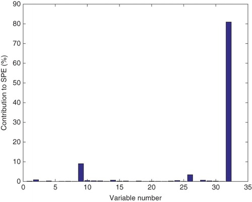
In this article, fault variables were identified using a sensitivity analysis principle (Petzold, Barbara, Tech, Li, Cao, & Serban, 2006). The method is based on calculating the rate of change in system output variables resulting from changes in the problem causing parameters (Deng, Tian, & Chen, 2013). Given a test data vector with n variables, the contribution of the variable to a monitoring index is defined by (27) where and . In this work, the partial derivatives were obtained by differentiating the functions defining and Q at a given reference fault instant using complex step differentiation (Martins, Sturdza, & Alonso, 2003). This is an efficient generalized approach for obtaining variable contributions in fault identification studies that use multivariate statistical methods.

3. Application

3.1. Tennessee Eastman process

The TE process is a simulation of a real industrial process manifesting both nonlinear and dynamic properties (Downs & Vogel, 1993). It is widely used as a benchmark process for evaluating and comparing process monitoring and control approaches (Chiang et al., 2001). The process consists of five key units: separator, compressor, reactor, stripper and condenser, and eight components coded A to H. The control structure of the process is presented in Figure 2.

Figure 2. Control structure of TE process.

There are 960 samples and 53 variables, which include 22 continuous variables, 19 composition measurements sampled by 3 composition analysers, and 12 manipulated variables in the TE process. Sampling is done at 3-minute intervals while each fault is introduced at sample number 160. Information on disturbances and baseline operating conditions of the process are documented in (Downs & Vogel, 1993; McAvoy & Ye, 1994).

3.2. Application procedure

Five hundred samples obtained under NOC were used as the training data set and all 960 samples obtained under each of the faulty operating conditions were used as test data. All 22 continuous variables and 11 manipulated variables were used in this study. The agitation speed of the reactor's stirrer (the 12th manipulated variable) was not included because it is constant. A total of 20 faults in the process were studied. Descriptions of the variables and faults studied are presented in Tables 3 and 4.

Table 3. TE process monitoring variables.

No.	Description	No.	Description
1	A feed (stream 1)	18	Stripper temperature
2	D feed (stream 2)	19	Stripper stream flow
3	E feed (stream 4)	20	Compressor work
4	Total feed (stream 4)	21	Reactor cooling water outlet temperature
5	Recycle flow (stream 8)	22	Condenser cooling water outlet temperature
6	Reactor feed rate (stream 6)	23	D feed flow (stream 2)
7	Reactor pressure	24	E feed flow (stream 3)
8	Reactor level	25	A feed flow (stream 1)
9	Reactor temperature	26	Total feed flow (stream 4)
10	Purge rate	27	Compressor recycle valve
11	Separator temperature	28	Purge valve
12	Separator level	29	Separator pot liquid flow (stream 10)
13	Separator pressure	30	Stripper liquid product flow
14	Separator under flow (stream 10)	31	Stripper steam valve
15	Stripper stream valve	32	Reactor cooling water flow
16	Stripper pressure	33	Condenser cooling water flow
17	Stripper under flow(stream 11)

Table 4. Fault descriptions in the TE process.

Fault	Description	Type
1	A/C feed ratio, B composition constant	Step
2	B composition, A/C ratio constant	Step
3	D feed temperature	Step
4	Reactor cooling water inlet temperature	Step
5	Condenser cooling water inlet temperature	Step
6	A feed loss	Step
7	C header pressure loss-reduced availability	Step
8	A, B, C feed composition	Random variation
9	D feed temperature	Random variation
10	C feed temperature	Random variation
11	Reactor cooling water inlet temperature	Random variation
12	Condenser cooling water inlet temperature	Random variation
13	Reaction kinetics	Slow drift
14	Reactor cooling water valve	Sticking
15	Condenser cooling water valve	Sticking
16	Unknown
17	Unknown
18	Unknown
19	Unknown
20	Unknown

Several methods have been proposed for determining the number of retained PCs. Some of these methods are scree tests, the average eigenvalue approach, cross-validation, parallel analysis, Akaike information criterion, and the cumulative percent eigenvalue. However, none of these methods have been proved analytically to be the best in all situations (Chiang et al., 2001). In this paper, the number of PCs that explained over 90% of the total variance were retained. Based on this approach, 16 and 17 PCs were selected for PCA and KPCA, respectively.

Another, important parameter for kernel-based methods in model development for process monitoring is the choice of kernel and its width. The radial basis kernel which is a common choice for process monitoring studies (Lee et al., 2004; Stefatos & Hamza, 2007) was used in this paper. The value of the kernel parameter c was determined using the relation , where W is a constant, which is dependent on the process being monitored, n and are the dimension and variance of the input space, respectively (Lee et al., 2004; Mika et al., 1999). The value of W was set at 40 with validation from the training data.

The and Q statistics were used jointly for fault detection due to their complementary nature. This means that a fault detection was acknowledged when either of the monitoring statistics detected a fault. This is because detectable process variation may not always occur in both the model space and the residual space at the same time.

3.3. Fault detection rule

Since measurements obtained from chemical processes are usually noisy, monitoring indices may exceed their thresholds randomly. This amounts to announcing the presence of a fault when no disturbance has actually occurred, that is, a false alarm. In other words, a monitoring index may exceed its threshold once but if no fault is present, the monitoring index may not stay above its threshold in subsequent measurements. Conversely, a fault has likely occurred if the monitoring index stays above its threshold in several consecutive measurements. A fault detection rule is used to address the problem of spurious alarms (Choi & Lee, 2004; Tien, Lin, & Jun, 2004; van Sprang, Ramaker, Westerhuis, Gurden, & Smilde, 2002). A detection rule also provides a uniform basis for comparing different monitoring methods. In this paper, successful fault detection was counted when a monitoring index exceeds its control limit in at least two consecutive observations. All algorithms recorded a false alarm rate (FAR) of zero when tested with the training data based on this criterion. Computation of the metrics for evaluating the monitoring performance of the different techniques was therefore based on this criterion.

3.4. Computation of monitoring performance metrics

Monitoring performance was based on three metrics: fault detection rates (FDRs), FARs, and detection delay. FDR is the percentage of fault samples identified correctly. It was computed as (28) where denotes the number of fault samples identified correctly and is the total number of fault samples. FAR was calculated as the percentage of normal samples identified as faults (or abnormal) during the normal operation of the plant. (29) where represents the number of normal samples identified as faults and is the total number of normal samples. Detection delay was computed as the time that elapsed before a fault introduced was detected.

3.5. Results and discussion

KPCA-based fault detection is demonstrated using Faults 11 and 12 of the TE process. Fault 11 is a random variation in the reactor cooling water inlet temperature, while Fault 12 is a random variation in the condenser cooling water inlet temperature. The monitoring charts for the two faults are shown in Figures 3 and  4, respectively. The solid curves represent the monitoring indices, while the dash-dot and dash lines represent the control limits at 99% confidence level based on Gaussian distribution and KDE, respectively. It can be seen that in both cases, especially in the control charts, the KDE-based control limits are below the Gaussian distribution-based control limits. That is, the monitoring indices exceed the KDE-based control limits to a greater extent compared to the Gaussian distribution-based control limits. This implies that using the KDE-based control limits with the KPCA technique gives higher monitoring performance compared to using the Gaussian distribution-based control limits.

Figure 3. Monitoring charts for Fault 11.

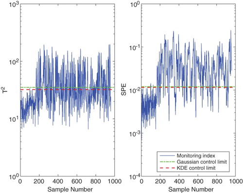
Figure 4. Monitoring charts for Fault 12.

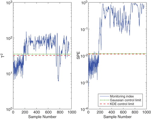
Table 5 shows the detection rates for PCA, PCA–KDE, KPCA, and KPCA–KDE for all 20 faults studied. The results show that the KDE versions have overall higher FDRs compared to the corresponding Gaussian distribution-based versions. Furthermore, in Table 6, it can be seen that the detection delays of the KDE-based versions are either equal to or lower than the non-KDE-based techniques. This implies that the approaches based on KDE-derived UCLs detected faults earlier than their Gaussian distribution-based counterparts. Thus, associating KDE-based control limits with the KPCA technique for fault detection provides better monitoring compared to using control limits based on the Gaussian assumption.

Table 5. Fault detection rates (%).

Fault	PCA	PCA–KDE	KPCA	KPCA–KDE
1	99.75	99.75	99.75	99.75
2	98.25	98.75	98.63	98.63
3	0.13	0.88	1.63	1.75
4	99.88	99.88	99.88	99.88
5	23.63	25.75	26.38	26.88
6	99.88	99.88	99.88	99.88
7	99.88	99.88	99.88	99.88
8	96.88	97.38	98.00	98.00
9	0.25	1.13	1.63	2.25
10	35.75	41.63	51.13	53.50
11	74.75	77.50	78.13	79.88
12	97.50	97.63	97.50	97.63
13	95.50	95.75	95.38	95.63
14	99.75	99.75	99.75	99.75
15	0	1.13	2.13	2.88
16	27.50	36.13	39.75	44.62
17	92.50	93.88	93.00	93.50
19	5.50	9.88	10.13	13.50
20	49.25	53.00	57.13	57.75

Table 6. Detection delay, DD (min).

Fault	PCA	PCA–KDE	KPCA	KPCA–KDE
1	6	6	6	6
2	39	30	33	33
3	2346	1656	1725	1725
4	3	3	3	3
5	3	3	3	3
6	3	3	3	3
7	3	3	3	3
8	48	48	48	48
9	2346	1665	1725	1725
10	186	186	180	180
11	15	15	15	15
12	42	30	60	42
13	102	102	111	105
14	6	6	6	6
15	ND	1656	1725	1725
16	81	78	81	81
17	45	45	45	45
18	24	24	24	24
19	213	24	213	36
20	105	102	105	105

Note: ND, not detected.

KPCA–KDE-based fault identification is demonstrated using Fault 11 as an example. The occurrence of Fault 11 induces change in the reactor cooling water flow rate, which causes the reactor temperature to fluctuate. Both the - and SPE-based contribution plots at sample 300 shown in Figures 5 and 6, respectively, identified the two fault variables correctly. Variable 9 is the reactor temperature while variable 32 corresponds to the reactor cooling water flow rate. Although it is possible for the control loops to compensate the change in the reactor temperature after a longer time has elapsed, the fluctuations in both variables affected early after the introduction of the fault were correctly identified by the contribution plots.

Figure 5. -based contribution plot for Fault 11.

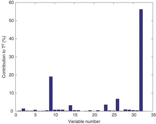
Figure 6. SPE-based contribution plot for Fault 11.

3.6. Test of robustness

To test the robustness of the KPCA–KDE technique, fault detection was performed by varying two parameters: bandwidth and the number of PCs retained. Figure 7 shows the monitoring charts for KPCA and KPCA–KDE with W=40 for Fault 14. This fault represents sticking of the reactor cooling water valve, which is quit easily detected by most statistical process monitoring approaches. At W=40, both KPCA and KPCA–KDE recoded zero false alarms (Figure 7). However, at W=10, KPCA recorded a false alarm rate of 8.13% while the FAR for KPCA–KDE was still zero (Figure 8). Also, Table 7 shows that the KPCA recorded a similar high FAR when 25 PCs were retained. Conversely, the KPCA–KDE approach still recorded zero false alarms.

Figure 7. KPCA-based control charts for Fault 14 at W=40 in the formula .

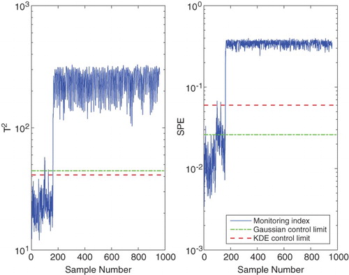
Figure 8. KPCA–KDE-based control charts for Fault 14 at W=10 in the formula .

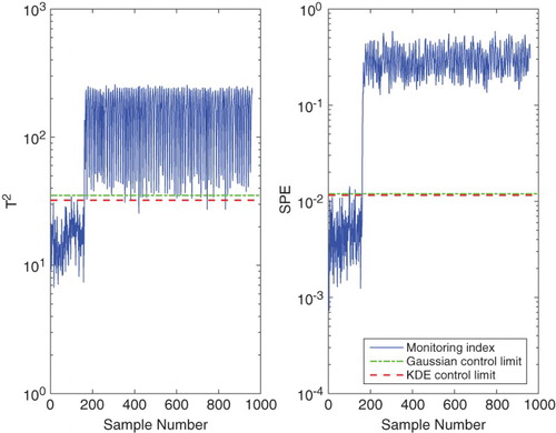
Table 7. Monitoring results at different number ofPCs retained.

	KPCA			KPCA–KDE
PCs	FDR	FAR	DD	FDR	FAR	DD
10	99.88	0	3	99.88	0	3
15	99.75	0	6	99.75	0	6
20	96.75	0	6	99.88	0	3
25	99.88	8.13	3	99.75	0	6

Thus, apart from generally providing higher FDRs and earlier detections, the KPCA–KDE is more robust than the KPCA technique with control limits based on the Gaussian assumption. A more sensitive technique is better for process operators since less faults will be missed. Secondly, when faults are detected early, operators will have more time to find the root cause of the fault so that remedial actions can be taken before a serious upset occurs. Thirdly, although methods are available for obtaining optimum design parameters for developing process monitoring models, there is no guarantee that the optimum values are used all the time. The reason for this may range from lack of experience of personnel to lack of or limited understanding of the process itself. Therefore, the more robust a technique is, the better it is for process operations.

4. Conclusion

This paper investigated nonlinear process fault detection and identification using the KPCA–KDE technique. In this approach, the thresholds used for constructing control charts were derived directly from the PDFs of the monitoring indices instead of using thresholds based on the Gaussian distribution. The technique was applied to the benchmark Tennessee Eastman process and its fault detection performance was compared with the KPCA technique based on the Gaussian assumption.

The overall results show that KPCA–KDE detected faults more and earlier than the KPCA with control limits based on the Gaussian distribution. The study also shows that the UCLs based on KDE are more robust than those based on the Gaussian assumption because the former follow the actual distribution of the monitoring statistics more closely. In general, the work corroborates the claim that using KDE-based control limits give better monitoring results in nonlinear processes than using control limits based on the Gaussian assumption. A generalizable approach for computing variable contributions in fault identification studies that centre on multivariate statistical methods was also demonstrated.

Disclosure statement

No potential conflict of interest was reported by the authors.

Additional information

Funding

The first author was supported by Bayelsa State Scholarship Board (Government of Bayelsa State of Nigeria) [BSSB/AD/ CON/VOL.1 PHD.006].

References

- Bowman, A. W., & Azzalini, A. (1977). Applied smoothing techniques for data analysis: The kernel approach with s-plus illustrations. Oxford: Clarendon Press.
- Chen, Q., Wynne, R. J., Goulding, P., & Sandoz, D. (2000). The application of principal component analysis and kernel density estimation to enhance process monitoring. Control Engineering Practice, 8(5), 531–543. doi: 10.1016/S0967-0661(99)00191-4
- Cheng, C., & Chiu M. -S. (2005). Non-linear process monitoring using JITL-PCA. Chemometrics Intelligent Laboratory Systems, 76, 1–13. doi: 10.1016/j.chemolab.2004.08.003
- Chiang, L., Russell, E., & Braatz, R. (2001). Fault detection and diagnosis in industrial systems. London: Springer-Verlag.
- Cho J. -H., Lee J. -M., Choi, S. W., Lee, D., & Lee I. -B. (2005). Fault identification for process monitoring using kernel principal component analysis. Chemical Engineering Science, 60(1), 279–288. doi: 10.1016/j.ces.2004.08.007
- Choi, S. W., & Lee I. -B. (2004). Nonlinear dynamic process monitoring based on dynamic kernel PCA. Chemical Engineering Science, 59, 5897–5908. doi: 10.1016/j.ces.2004.07.019
- Choi, S. W., Lee, C., Lee J. -M., Park, J. H., & Lee I. -B. (2005). Fault detection and identification of nonlinear processes based on kernel PCA. Chemometrics and Intelligent Laboratory Systems, 75, 55–67. doi: 10.1016/j.chemolab.2004.05.001
- Deng, X., Tian, X., & Chen, S. (2013). Modified kernel principal component analysis based on local structure analysis and its application to nonlinear process fault diagnosis. Chemometrics and Intelligent Laboratory Systems, 127(15), 195–209. doi: 10.1016/j.chemolab.2013.07.001
- Dong, D., & McAvoy, T. J. (1996). Non-linear principal component analysis-based on principal curves and neural networks. Computers and Chemical Engineering, 20(1), 65–78. doi: 10.1016/0098-1354(95)00003-K
- Downs, J., & Vogel, E. (1993). A plant-wide industrial process control problem. Computers and Chemical Engineering, 17(3), 245–255. doi: 10.1016/0098-1354(93)80018-I
- Ge, Z., & Song, Z. (2013). Multivariate statistical process control: Process monitoring methods and applications. London: Springer-Verlag.
- Ge, Z., Song, Z., & Gao, F. (2013). Review of recent research on data-based process monitoring. Industrial and Engineering Chemistry Research, 52, 3543–3562. doi: 10.1021/ie302069q
- Hiden, H. G., Willis, M. J., Tham, M. T., & Montague, G. A. (1999). Nonlinear principal component analysis using genetic programming. Computers and Chemical Engineering, 23, 413–425. doi: 10.1016/S0098-1354(98)00284-1
- Jackson, J. (1991). A user's guide to principal components. New York, NY: Wiley.
- Jia, F., Martin, E. B., & Morris, A. J. (2000). Non-linear principal components analysis with application to process fault detection. International Journal of Systems Science, 31(11), 1473–1487. doi: 10.1080/00207720050197848
- Jolliffe, I. (2002). Principal component analysis (2nd ed). New York, NY: Springer-Verlag.
- Kramer, M. A. (1992). Autoassociative neural networks. Computers and Chemical Engineering, 16(4), 313–328. doi: 10.1016/0098-1354(92)80051-A
- Kruger, U., Antory, D., Hahn, J., Irwin, G. W., & McCullough, G. (2005). Introduction of a nonlinearity measure for principal component models. Computers and Chemical Engineering, 29(11–12), 2355–2362. doi: 10.1016/j.compchemeng.2005.05.013
- Lee J. -M., Yoo, C. K., Choi, S. W., Vanrolleghem, P. A., & Lee I. -B. (2004). Nonlinear process monitoring using kernel principal component analysis. Chemical Engineering Science, 59, 223–234. doi: 10.1016/j.ces.2003.09.012
- Liang, J. (2005). Multivariate statistical process monitoring using kernel density estimation. Developments in Chemical Engineering and Mineral Processing, 13(1–2), 185–192. doi: 10.1002/apj.5500130117
- Martins, J. R. R. A., Sturdza, P., & Alonso, J. J. (2003). The complex-step derivative approximation. ACM Transaction on Mathematical Software, 29(3), 245–262. doi: 10.1145/838250.838251
- McAvoy T. J., & Ye, N. (1994). Base control for the Tenessee Eastman problem. Computers and Chemical Engineering, 18, 383–413. doi: 10.1016/0098-1354(94)88019-0
- Mika, S., Schölkopf, B., Smola, A., Müller, K. R., Scholz, M., & Rätsch, G. (1999). Kernel PCA and de-noising in feature spaces. Advances in Neural Information Processing System, 11, 536–542.
- Odiowei P. E. P., & Cao, Y. (2010). Nonlinear dynamic process monitoring using canonical variate analysis and kernel density estimations. IEEE Transactions on Industrial Informatics, 6(1), 36–44. doi: 10.1109/TII.2009.2032654
- Petzold, L., Barbara, S., Tech, V., Li, S., Cao, Y., & Serban, R. (2006). Sensitivity analysis of differential-algebraic equations and partial differential equations. Computers & Chemical Engineering, 30(10–12), 1553–1559. doi: 10.1016/j.compchemeng.2006.05.015
- Russell, E., Chiang, L., & Braatz, R. (2000). Data-driven methods for fault detection and diagnosis in chemical processes. London: Springer-Verlag.
- Schölkopf B., Smola, A. J., & Müller K.-R. (1998). Non-linear component analysis as a kernel eigenvalue problem. Neural Computation, 10(5), 1299–1399. doi: 10.1162/089976698300017467
- van Sprang, E. N. M., Ramaker H. -J., Westerhuis, J. A., Gurden, S. P., & Smilde, A. K. (2002). Critical evaluation of approaches for on-line batch process monitoring. Chemical Engineering Science, 57(18), 3979–3991. doi: 10.1016/S0009-2509(02)00338-X
- Stefatos, G., & Hamza, A. B. (2007). Statistical process control using kernel PCA. 15th Mediterranean Conference on Control and Automation, Anthens, Greece, 1418–1423.
- Tien, D. X., Lin, K. W., & Jun, L. (2004). Comparative study of PCA approaches in process monitoring and fault detection. 30th Annual Conference on the IEEE Industrial Electronic Society, November 2-6, Busan Korea, 2594–2599.
- Wise B. M., & Gallagher N . B. (1996). The process chemometrics approach to process monitoring and fault detection. Journal of Process Control, 6, 329–348. doi: 10.1016/0959-1524(96)00009-1
- Wold, S., Esbensen, K., & Geladi, P. (1987). Principal component analysis. Chemometrics and Intelligent Laboratory Systems, 2(1–3), 37–52. doi: 10.1016/0169-7439(87)80084-9
- Xiong, L., Liang, J., & Qian, J. (2007). Multivariate statistical monitoring of an industrial polypropylene catalyser reactor with component analysis and kernel density estimation. Chinese Journal of Engineering, 15(4), 524–532. doi: 10.1016/S1004-9541(07)60119-0
- Yin, S., Ding, S. X., Xie, X. S., & Luo, H. (2014). A review on basic data-driven approaches for industrial process monitoring. IEEE Transactions on Industrial Electronics, 61(11), 6418–6428. doi: 10.1109/TIE.2014.2301773
- Yin, S., Li, X., Gao, H., & Kaynak, O. (2015). Data-based techniques focused on modern industry: An overview. IEEE Transactions on Industrial Electronics, 62(1), 657–667. doi: 10.1109/TIE.2014.2308133