The paradigm of complex probability and analytic nonlinear prognostic for vehicle suspension systems

ABSTRACT

Adding three novel axioms to Kolmogorov's five established probability axioms which were laid in 1933 extends classical probability theory to encompass the imaginary set of numbers. Therefore, all random experiments will be executed in the complex set which is the sum of the real set with its real probability component, and the corresponding imaginary set with its imaginary probability component. The purpose of extending Kolmogorov's axioms is to add supplementary imaginary dimensions to any random event that occurs in the ‘real’ laboratory and hence to be able to evaluate the associated complex probability in the complex plane which is always equal to one. My purpose in this work is to link the complex probability paradigm to the vehicle suspension system analytic prognostic in the nonlinear damage accumulation case. Hence, by calculating the parameters of the new prognostic model, we will be able to determine the magnitude of the chaotic factor, the degree of our knowledge, the complex probability, the system failure and survival probabilities, and the remaining useful lifetime probability, after that N load cycles have been applied to the suspension, and which are all functions of the system degradation subject to random effects.

KEYWORDS:

• Complex set
• probability norm
• degree of our knowledge
• chaotic factor
• nonlinear damage
• degradation
• remaining useful lifetime
• prognostic

Nomenclature

	=	real probability set of events
	=	imaginary probability set of events
	=	complex probability set of events
i	=	the imaginary number where
EKA	=	extended Kolmogorov's axioms
CPP	=	complex probability paradigm
Prob	=	probability of any event
Pr	=	probability in the real set  = system failure probability
Pm	=	probability in the imaginary set corresponding to the real probability in  = system survival probability
Pm/i	=	probability in the set corresponding to the imaginary probability in
Pc	=	probability of an event in with its associated event in , it is the probability in the complex set
Z	=	complex probability number and vector, it is the sum of Pr and Pm
DOK	=	= degree of our knowledge of the random experiment and event, it is the square of the norm of Z.
Chf	=	chaotic factor
MChf	=	magnitude of the chaotic factor
N	=	number of load cycles
NC	=	number of load cycles till system failure
	=	load amplitude mean in one cycle
fj(N)	=	probability density function for each road mode j
F(N)	=	cumulative distribution function
ψ	=	simulation magnifying factor
D	=	degradation indicator of a system
RUL	=	remaining useful lifetime of a system
Prob[RUL(N)]	=	probability of RUL after N load cycles

1. Introduction

Firstly, let us present in this section an overview of probability theory history. The scientific study of probability is a modern development of mathematics. In fact, there has been an interest in quantifying the ideas of probability for millennia as a result of the widespread of gambling, however, exact mathematical descriptions appeared much later. The development of the mathematics of probability was slow due to many reasons: although games of chance provided the motivation for the mathematical study of probability, fundamental issues were still obscured by the gamblers’ superstitions (Freund, 1973; Kuhn, 1970; Poincaré, 1968; Stewart, 1996; Wikipedia, Probability). Richard Jeffrey indicated that:

Before the middle of the seventeenth century, the term ‘probable’ (Latin probabilis) meant approvable, and was applied in that sense, univocally, to opinion and to action. A probable action or opinion was one such as sensible people would undertake or hold, in the circumstances. (1992)

However, the word ‘probable’, in legal contexts especially, could also apply to propositions for which there was good evidence (Stewart, 2012; Warusfel & Ducrocq, 2004).

In the sixteenth century, Gerolamo Cardano, the Italian polymath, efficiently defined odds as the ratio of favourable to unfavourable outcomes. This implies that the probability of an event is given by the ratio of favourable outcomes to the total number of possible outcomes (Gorrochum, 2012). Besides Cardano's elementary work, the correspondence of Pierre de Fermat and Blaise Pascal in 1654 initiated the doctrine of probabilities. In 1657 precisely, the earliest known scientific treatment of the subject was provided by Christiaan Huygens (Abrams). The subject was treated as a branch of mathematics in 1713 by Jakob Bernoulli (posthumously) in his Ars conjectandi and in 1718 by Abraham de Moivre in his Doctrine of chances (Ivancevic & Ivancevic, 2008). For the history of the early development of the very concept of mathematical probability, one can refer to the work of Ian Hacking entitled The emergence of probability (Hacking, 2006), and of James Franklin named The science of conjecture (Barrow, 1992; Franklin, 2001; Greene, 2003; Hawking, 2005).

In 1722, Roger Cotes (posthumously) in his Opera miscellanea discussed the theory of errors. However, in 1755, Thomas Simpson was the first to apply the theory to the discussion of errors of observation in his memoir which was printed in 1756. The axioms that positive and negative errors are equally probable, and that certain assignable limits define the range of all errors, were laid down in the reprint of this memoir in 1757. Continuous errors and a description of a probability curve were also discussed by Simpson (Bogdanov & Bogdanov, 2012, 2013; Penrose, 1999). Moreover, Marquis Pierre-Simon de Laplace proposed the two laws of error. The first law stated that the frequency of an error could be expressed as an exponential function of the numerical magnitude of the error, disregarding sign and was published in 1774. The second law of error stated that the frequency of the error is an exponential function of the square of the error and was proposed by Laplace in 1778 (Wilson, 1923). The second law of error is called the normal distribution or the Gauss law. ‘It is difficult historically to attribute that law to Gauss, who in spite of his well-known precocity had probably not made this discovery before he was two years old’ (Bogdanov & Bogdanov, 2009, 33, 2010, 49).

The principle of the maximum product of the probabilities of a system of concurrent errors was introduced in 1778 by Daniel Bernoulli. The method of least squares was developed and introduced by Adrien-Marie Legendre in 1805 in his Nouvelles méthodes pour la détermination des orbites des comètes (New methods for determining the orbits of comets) (Seneta, 2016). Robert Adrain who is an Irish-American writer and the editor of ‘The analyst’ ignored Legendre's contribution, and first deduced in 1808 the law of facility of error, where c is a constant depending on the precision of observation, and h is a scale factor ensuring that the area under the curve equals 1. Adrain gave two proofs of this law. The second proof is essentially similar to the proof given by John Herschel in 1850. The first proof was given by Gauss and it seems to have been known in Europe in 1809 (the third after Adrain's). Further proofs were given by Laplace in 1810 and 1812, Gauss in 1823, James Ivory in 1825 and 1826, Hagen in 1837, Friedrich Bessel in 1838, W. F. Donkin in 1844 and 1856, and Morgan Crofton in 1870. Other contributors were Ellis in 1844, De Morgan in 1864, Glaisher in 1872, and Giovanni Schiaparelli in 1875. In 1856, Peters's formula for r, the probable error of a single observation, is well known (Davies, 1993; Wikipedia, Probability density function; Wikipedia, Probability space).

The probability general theory was developed in the nineteenth century by authors such as Laplace, Sylvestre Lacroix in 1816, Littrow in 1833, Adolphe Quetelet in 1853, Richard Dedekind in 1860, Helmert in 1872, Hermann Laurent in 1873, Liagre, Didion, and Karl Pearson. The exposition of the theory was improved by Augustus De Morgan and George Boole (Wikipedia, Probability axioms; Wikipedia, Probability measure). In 1906, the notion of Markov chains was introduced by Andrey Markov (http://www.statslab.cam.ac.uk/∼rrw1/markov/M.pdf). This notion played an essential role in the theory of stochastic processes and its applications. In 1931, Andrey Kolmogorov, developed ‘measure theory’ which is the basis of the modern theory of probability (Vitanyi, 1988). Like other theories,

the theory of probability is a representation of probabilistic concepts in formal terms – that is, in terms that can be considered separately from their meaning. These formal terms are manipulated by the rules of mathematics and logic, and any results are interpreted or translated back into the problem domain. (Wikipedia, Probability theory)

There have been at least two successful attempts to formalise probability, namely the Kolmogorov formulation and the Cox formulation.

In Kolmogorov’s formulation, sets are interpreted as events and probability itself as a measure on a class of sets. In Cox’s theorem, probability is taken as a primitive (that is, not further analyzed) and the emphasis is on constructing a consistent assignment of probability values to propositions. In both cases, the laws of probability are the same, except for technical details. (Hawking, 2011; Wikipedia, Probability distribution)

Uncertainty can be quantified by other methods such as the Dempster–Shafer theory or possibility theory. However, those two theories are essentially different and are not compatible with the laws of probability as usually understood (Aczel, 2000; Hawking, 2002).

Based on Sir Isaac Newton's concepts, we understand that in a deterministic universe there would be no probability if all conditions were known (Laplace's demon). However, there are situations in which sensitivity to initial conditions exceeds our ability to measure them, that is, to know them. In the case of a roulette wheel, if the force of the hand and the period of that force are known, the number on which the ball will stop would be a certainty. However, as Thomas A. Bass' Newtonian Casino revealed and as a practical matter, this would likely be true only of a roulette wheel that had not been exactly levelled. Certainly, knowledge of inertia and friction of the wheel, weight, smoothness and roundness of the ball, variations in hand speed during the turning and so forth were also assumed. Hence, a probabilistic description can be more useful than Newtonian mechanics for analyzing the pattern of outcomes of repeated rolls of a roulette wheel. The same situation is faced by physicists in the kinetic theory of gases. As a matter of fact, the system, while deterministic in principle, is so complex that only a statistical description of its properties is feasible. Actually, the number of molecules is typically of the order of magnitude of Avogadro's constant which is nearly equal to 6.02 × 10²³ (Boltzmann, 1995; Cercignani, 2010; Pickover, 2008; Planck, 1969; Reeves, 1988; Ronan, 1988).

Furthermore, the description of quantum phenomena requires probability theory (Burgi, 2010). The random character of all physical processes that occur at sub-atomic scales and which are governed by the laws of quantum mechanics was a revolutionary discovery of early twentieth-century physics. The objective wave function evolves deterministically. Nevertheless, according to the Copenhagen interpretation, it deals with probabilities of observing. The experiment outcome is being explained by a wave function collapse when an observation is made. However, the loss of determinism for the sake of instrumentalism did not meet with universal approval. Albert Einstein famously remarked in a letter to Max Born: ‘I am convinced that God does not play dice’ (Jedenfalls bin ich überzeugt, 1916–1955). Like Einstein, Erwin Schrödinger, who discovered the wave function, believed that quantum mechanics is a statistical approximation of an underlying deterministic reality (Moore, 1992). In some modern interpretations of the statistical mechanics of measurement, quantum decoherence is invoked to account for the appearance of subjectively probabilistic experimental outcomes (Balibar, 2002; Hoffmann, 1975).

Secondly, let us introduce in this section also prognostic theory as well as my adopted model. Recent developments in system design technology such as in aerospace, defense, petro-chemistry, and automobiles are represented earlier in the literature by simulated models during the conception step and this is to ensure the high availability of the industrial systems. Knowing that, the integration of diagnostic–prognostic models in these industrial systems is facilitated by these developments. In fact, the monitoring of the degradation indicators is used indirectly in failure prognostic and is just a measurement of an unwanted situation. Therefore, the diagnostic is not only a failure detection procedure but it also indicates the actual state and the historic of the system. Hence, a predictive maintenance was done by my previous prognostic model (Abou Jaoude, El-Tawil, Kadry, Noura, & Ouladsine, 2010, 2011; El-Tawil, Abou Jaoude, Kadry, Noura, & Ouladsine, 2010; El-Tawil, Kadry, & Abou Jaoude, 2009). Consequently, from a predefined threshold of degradation, the remaining useful lifetime (RUL) was estimated. Based on a physical dynamic vehicle suspension system, my research work elaborated a procedure to create a failure prognostic model that will be more developed and further improved in the current paper.

Prognostic is a methodology that aims to predict the RUL of a system in service. RUL can be expressed in hours of functioning, in kilometers run or in cycles. Vachtsevanos et al. (2006) define prognostics as the ability to ‘predict and prevent’ possible fault or system degradation before failures occur. Prognosis has been defined by Lemaitre and Chaboche (1990) as ‘prediction of when a failure may occur’, that is, a mean to calculate the remaining useful life of an asset. If we can effectively predict the condition of machines and systems, maintenance actions can be taken ahead of time. In order to make a good and reliable prognosis, it must have a good and reliable diagnosis (Abou Jaoude, El-Tawil, Kadry, Noura, & Ouladsine, 2011). Furthermore, in prognostic theory, it is well known that each system passes by three phases during its whole life. The last phase represents the degradation period of the system and which leads to failure by progressive deterioration. It is important for industrialists to predict, at each instant, the remaining lifetime in order to prevent expensive and unexpected failure. Early detection also helps in avoiding catastrophic failures. Adopting preventive systematic maintenance to increase the system availability proves to be an expensive strategy due to the frequent replacement of generally expensive accessories. This strategy is not efficient because most of equipment failures are not related only to the number of hours of functioning (Abou Jaoude, Noura, El-Tawil, Kadry, & Ouladsine, 2012a, 2012b).

Moreover, I introduced a prognostic approach that seeks to provide an intelligent maintenance. A proposed analytic prognostic methodology based on some laws of damage in fracture mechanics was developed (Abou Jaoude, 2012). The damages are generally: crack propagation, corrosions, chloride attack, creep, excessive deformation and deflection, and damage accumulation. Whenever their analytic laws are available, the advantage of a prognostic approach based on a known damage law for a mechanical system is that it is adaptable to new situations and useful in determining the RUL of the system. In fact, any prognostic methodology must lie on a type of damage. In my research work, the case of fatigue degradation has been chosen due to the fact that it can be mathematically formulated by the analytic Paris–Erdogan's law. A degradation indicator D was taken to describe the evolution from an initial micro-damage till the total system failure. Additionally, damages have been assumed by many researchers to accumulate linearly (Palmgren–Miner's law) even though it is unlikely to be the case of brittle material. In my previous paper (Abou Jaoude & El-Tawil, 2013a), I explored the nonlinear side of cumulative damage to take into account the nature of the applied constraints and influent environment that can accentuate the nonlinear aspect related to some materials behaviour subject to fatigue effects (Abou Jaoude & El-Tawil, 2013b; El-Tawil & Abou Jaoude, 2013).

The procedure proposed in all my work belongs to the model-based prognosis approach related to the physical model. It is focused on developing and implementing effective diagnostic and prognostic technologies with the ability to detect faults in the early stages of degradation. Early detection and analysis may lead to better prediction and end-of-life estimations by tracking and modelling the degradation process. The idea is to use these estimations to make accurate and precise prediction of the time to failure of components (Abou Jaoude, 2013a, 2015a).

Thirdly and finally, this research paper is organised as follows: After the introduction in Section 1, the purpose and the advantages of the present work are presented in Section 2. Afterward, in Section 3, I explain and illustrate the extended Kolmogorov's axioms and hence the complex probability paradigm (CPP), with their original parameters and interpretation. In Section 4, my published analytic prognostic model of fatigue for vehicle suspension systems in the nonlinear cumulative damage case is recapitulated. Moreover, in Section 5, the CPP new and basic assumptions are laid down, elaborated, and applied to analytic nonlinear prognostic. Furthermore, the simulations of the novel model for the three road conditions and modes are illustrated in Section 6. Finally, I conclude the work by doing a comprehensive summary in Section 7, and then present the list of references cited in the current research work.

2. The purpose and the advantages of the present work

All our work in classical probability theory is to compute probabilities. The original idea in this paper is to add new dimensions to our random experiment which will make the work totally deterministic. In fact, probability theory is a nondeterministic theory by nature, which means that the outcome of the stochastic events is due to chance and luck. By adding new dimensions to the event occurring in the ‘real’ laboratory which is , we make the work deterministic and hence a random experiment will have a certain outcome in the complex set of probabilities . It is of great importance that the stochastic system becomes totally predictable since we will be perfectly knowledgeable to foretell the outcome of chaotic and random events that occur in nature for example in statistical mechanics, in all stochastic processes, or in the well-established field of prognostic. Therefore, the work that should be done is to add to the real set of probabilities , the contributions of which is the imaginary set of probabilities that will make the event in absolutely deterministic. If this is found to be fruitful, then a new theory in stochastic sciences and prognostic would be elaborated and this is to understand deterministically those phenomena that used to be random phenomena in . This is what I called ‘The Complex Probability Paradigm’ that was initiated and elaborated in my seven previous papers (Abou Jaoude, 2013b, 2013c, 2014, 2015b, 2015c, 2016; Abou Jaoude, El-Tawil, & Kadry, 2010).

Moreover, although the analytic nonlinear prognostic laws are deterministic and very well known in Abou Jaoude and El-Tawil (2013a) but there are random and chaotic factors (such as temperature, humidity, applied load location, and water action) that affect the system and make its degradation function deviate from its calculated trajectory predefined by these deterministic laws. An updated follow-up of the degradation behaviour with time or cycle number, and which is subject to chaotic and non-chaotic effects, is done by what I called the system failure probability due to its definition that evaluates the jumps in the degradation function D.

Furthermore, my purpose in this current work is to link the CPP to the vehicle suspension system analytic prognostic in the nonlinear damage accumulation case. In fact, the system failure probability derived from prognostic will be included in and applied to the CPP. This will lead to the novel and original prognostic model illustrated in this paper. Hence, by calculating the parameters of the new prognostic model, we will be able to determine the magnitude of the chaotic factor (MChf), the degree of our knowledge (DOK), the complex probability, the system failure and survival probabilities, and the RUL probability, after that N load cycles have been applied to the suspension, and which are all functions of the system degradation subject to chaos and random effects.

Consequently, to summarise, the objectives and the advantages of the present work are to:

1. Extend classical probability theory to the set of complex numbers, hence to relate probability theory to the field of complex analysis in mathematics. This task was initiated and elaborated in my seven previous papers.

2. Do an updated follow-up of the degradation D behaviour with time or cycle number which is subject to chaos. This follow-up is accomplished by the system real failure probability due to its definition that evaluates the jumps in D; and hence, to relate probability theory to a system degradation in an original and a new way.

3. Apply the new probability axioms and paradigm to prognostic; thus, I will extend the concepts of prognostic to the complex probability set .

4. Prove that any random and stochastic phenomenon can be expressed deterministically in the complex set .

5. Quantify both the DOK and the chaos magnitude of the system degradation and its RUL.

6. Draw and represent graphically the functions and parameters of the novel paradigm associated with a suspension prognostic.

7. Show that the classical concepts of random degradation and RUL have a probability of occurring always equal to 1 in the complex set; hence, no chaos, no disorder, and no ignorance exist in (complex set) =  (real set) +  (imaginary set).

8. Prove that by adding supplementary and new dimensions to any random experiment whether it is a suspension system or any other stochastic system, we will be able to do prognostic in a deterministic way in the complex set .

9. Pave the way to apply the original paradigm to other topics in statistical mechanics, in stochastic processes, and to the field of prognostics in engineering. These will be the subjects of my subsequent research papers.

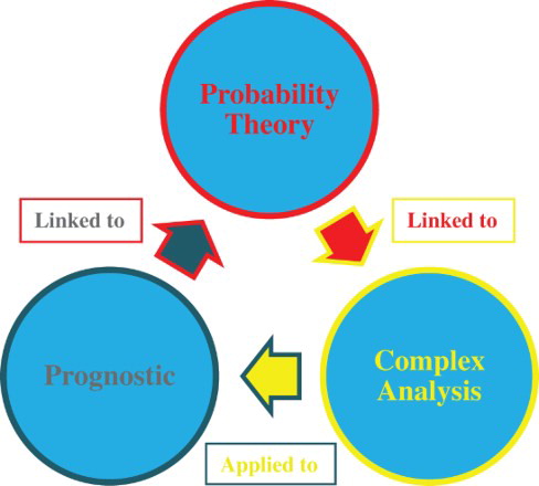
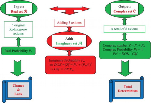
To conclude, compared with existing literature, the main contribution of this research paper is to apply the original CPP to the concepts of random degradation and RUL of a vehicle suspension system thus to the field of analytic prognostic in the nonlinear damage accumulation case. Figure 1 summarises the objectives of the current research paper.

Figure 1. The diagram of the principal objectives of this research work.

3. The extended set of probability axioms

In this section, I will present the extended set of probability axioms of the CPP.

3.1. The original Andrey N. Kolmogorov set of axioms

The simplicity of Kolmogorov's system of axioms may be surprising. Let E be a collection of elements {E₁, E₂, … } called elementary events and let F be a set of subsets of E called random events. The five axioms for a finite set E are as follows (Benton, 1966, 1966b; Feller, 1968; Montgomery & Runger, 2003; Walpole, Myers, Myers, & Ye, 2002):

• Axiom 1. F is a field of sets.

• Axiom 2. F contains the set E.

• Axiom 3. A non-negative real number P_rob(A), called the probability of A, is assigned to each set A in F. We have always 0 ≤ P_rob(A) ≤ 1.

• Axiom 4. P_rob(E) equals 1.

• Axiom 5. If A and B have no elements in common, the number assigned to their union is:

hence, we say that A and B are disjoint; otherwise, we have And we say also that which is the conditional probability. If both A and B are independent, then: .

Moreover, we can generalise and say that for N disjoint (mutually exclusive) events (for ), we have the following additivity rule:

And we say also that for N independent events (for ), we have the following product rule:

3.2. Adding the imaginary part

Now, we can add to this system of axioms an imaginary part such that

• Axiom 6. Let be the probability of an associated event in (the imaginary part) to the event A in (the real part). It follows that , where i is the imaginary number with .

• Axiom 7.  We construct the complex number or vector having a norm such that .

• Axiom 8. Let Pc denote the probability of an event in the complex probability universe , where . We say that Pc is the probability of an event A in with its associated event in such that

We can see that the system of axioms defined by Kolmogorov could be hence expanded to take into consideration the set of imaginary probabilities by adding three new axioms (Abou Jaoude, 2013b, 2013c, 2014, 2015b, 2015c, 2016; Abou Jaoude, El-Tawil, & Kadry, 2010).

3.3. The purpose of extending the axioms

It is apparent from the set of axioms that the addition of an imaginary part to the real event makes the probability of the event in always equal to 1. In fact, if we begin to see the set of probabilities as divided into two parts, one is real and the other is imaginary, understanding will follow directly. The random event that occurs in the real probability set (like tossing a coin and getting a head) has a corresponding probability . Now, let be the set of imaginary probabilities and let be the DOK of this phenomenon. is always, and according to Kolmogorov's axioms, the probability of an event.

A total ignorance of the set makes: and in this case is equal to: .

Conversely, a total knowledge of the set in makes: and . Here, we have because the phenomenon is totally known, that is, its laws and variables are completely determined; hence, our DOK of the system is 1=100%.

Now, if we can tell for sure that an event will never occur, that is, like ‘getting nothing’ (the empty set), is accordingly = 0, that is the event will never occur in . will be equal to: , and , because we can tell that the event of getting nothing surely will never occur; thus, the DOK of the system is 1=100% (Abou Jaoude, El-Tawil, & Kadry, 2010).

We can infer that we have always: and (1) And what is important is that in all cases we have (2)

In fact, according to an experimenter in , the game is a game of chance: the experimenter does no't know the output of the event. He will assign to each outcome a probability and he will say that the output is nondeterministic. But in the universe , an observer will be able to predict the outcome of the game of chance since he takes into consideration the contribution of , so we write: Hence, is always equal to 1. In fact, the addition of the imaginary set to our random experiment resulted in the abolition of ignorance and indeterminism. Consequently, the study of this class of phenomena in is of great usefulness since we will be able to predict with certainty the outcome of experiments conducted. In fact, the study in leads to unpredictability and uncertainty. So instead of placing ourselves in , we place ourselves in then study the phenomena, because in the contributions of are taken into consideration and therefore a deterministic study of the phenomena becomes possible. Conversely, by taking into consideration the contribution of the set , we place ourselves in and by ignoring we restrict our study to nondeterministic phenomena in (Bell, 1992; Boursin, 1986; Dacunha-Castelle, 1996; Srinivasan & Mehata, 1988; Stewart, 2002; Van Kampen, 2006).

Moreover, it follows from the above definitions and axioms that (Abou Jaoude, El-Tawil, & Kadry, 2010) (3) will be called the chaotic factor in our experiment and will be denoted accordingly by ‘Chf’. We will see why I have called this term the chaotic factor; in fact:

• In case , that is the case of a certain event, then the chaotic factor of the event is equal to 0.

• In case , that is the case of an impossible event, then Chf = 0. Hence, in both two cases, there is no chaos since the outcome is certain and is known in advance.

• In case , (Figures 2 and 3).

Figure 2. Chf, DOK, and Pc for the uniform probability distribution in 2D.

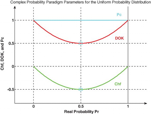
Figure 3. DOK, Chf, and Pc for the uniform probability distribution in 3D with .

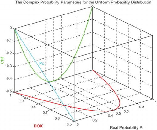
We notice that .

What is interesting here is thus we have quantified both the DOK and the chaotic factor of any random event and hence we write now: (4) Then we can conclude that therefore .

This directly means that if we succeed to subtract and eliminate the chaotic factor in any random experiment, then the output will always be with a probability equal to 1 (Dalmedico-Dahan, Chabert, & Chemla, 1992; Dalmedico-Dahan & Peiffer, 1986; Ekeland, 1991; Gleick, 1997; Gullberg, 1997; Science Et Vie, 1999).

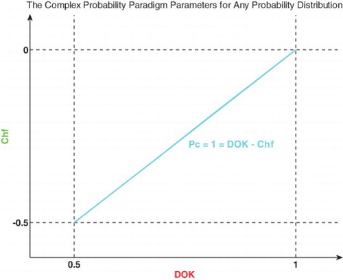
Figure 4 shows the linear relation between both DOK and Chf.

Figure 4. Graph of for any distribution

Furthermore, we need in our current study the absolute value of the chaotic factor that will give us the magnitude of the chaotic and random effects on the studied system materialised by the random cycle number N and a probability density function (PDF), and which lead to an increasing system chaos in and sometimes to a premature system failure. This new term will be denoted accordingly MChf (Abou Jaoude, 2015b, 2015c, 2016). Hence, we can deduce the following: (5) And

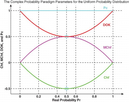
Figure 5 shows the linear relation between both DOK and MChf. Moreover, Figures 6–10 show the graphs of Chf, MChf, DOK, and Pc as functions of the real probability P_r for a uniform probability distribution.

Figure 5. Graph of for any distribution.

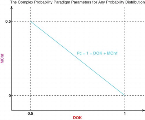
Figure 6. MChf, DOK, and Pc for the uniform probability distribution in 2D.

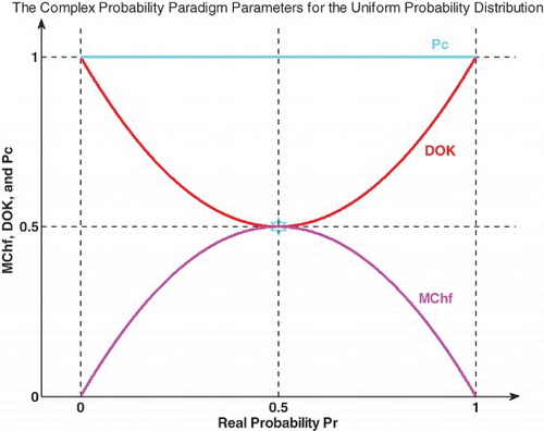
Figure 7. DOK, MChf, and Pc for the uniform probability distribution in 3D with .

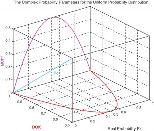
Figure 8. Chf and MChf for the uniform probability distribution in 2D.

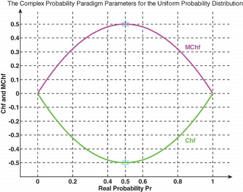
Figure 9. Chf and MChf for the uniform probability distribution in 3D with MChf + Chf = 0.

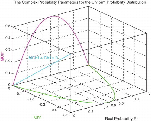
Figure 10. Chf, MChf, DOK, and Pc for the uniform probability distribution in 2D.

To summarise and to conclude, as the degree of our certain knowledge in the real universe is unfortunately incomplete, the extension to the complex set includes the contributions of both the real set of probabilities and the imaginary set of probabilities . Consequently, this will result in a complete and perfect degree of knowledge in (since Pc = 1). In fact, in order to have a certain prediction of any random event, it is necessary to work in the complex set in which the chaotic factor is quantified and subtracted from the computed degree of knowledge to lead to a probability in equal to one (Pc² = DOK − Chf = DOK + MChf = 1). This hypothesis is verified in my seven previous research papers by the mean of many examples encompassing both discrete and continuous distributions (Abou Jaoude, 2013b, 2013c, 2014, 2015b, 2015c, 2016; Abou Jaoude, El-Tawil, & Kadry, 2010). The extended Kolmogorov axioms (EKA for short) or the CPP can be illustrated in Figure 11:

Figure 11. The EKA or the CPP diagram.

4. Previous research work: analytic prognostic and nonlinear damage accumulation

I will do in this section a comprehensive summary of my previously published paper (Abou Jaoude & El-Tawil, 2013a) and I will just cite the results that this current article needs.

4.1. A brief introduction to the adopted methodology (Abou Jaoude & El-Tawil, 2013a)

The purpose of my previous research work, that will be improved in the current paper and will be related to CPP, was to create an analytic model of prognostic capable of predicting the degradation D and the RUL trajectories of a vehicle suspension system under a given environment and starting from an initial known damage.

The fatigue failure is one of the famous damage phenomena in mechanical systems like in vehicles where the suspension systems are subject to the fluctuation of roads stresses and loads . This type of loadings leads to a crack propagation that can accelerate rapidly. Usually, micro-cracks exist originally in the materials due to the fabrication process where stresses remain after manufacture. These micro-cracks are detected, measured, and denoted by a₀. The advantage of the choice of fatigue damage for my developed prognostic methodology is that it is a failure mechanism very well studied in the literature and described under many known analytic laws such as the very well-known damage law of Paris–Erdogan. This mechanism has relatively the simplest formulation in comparison to other damage phenomena. Knowing that, fatigue characterises the main failure cause of industrial equipment.

Furthermore, an indicator of degradation that varies from zero to one was derived. My proposed model was based on the link between this indicator D and the crack length a. Knowing that, failure occurs when a reaches a critical length after N_C critical load cycles. Hence, my model was given by a simple function relating the instantaneous degradation to actual crack length as a measurement of actual damage after N load cycles.

Furthermore, the aim was to evaluate the evolution of the system lifetime at each instant. For this purpose, the degradation trajectories had been used in terms of cycles' number or the time of operation. From these degradation trajectories, the RULs’ variations were deduced. Therefore, to demonstrate the effectiveness of my model, many industrial examples had been considered in the model simulation in these previous research papers and work (Abou Jaoude, 2012, 2013a, 2015a; Abou Jaoude & El-Tawil, 2013a, 2013b; Abou Jaoude, El-Tawil, Kadry, Noura, et al., 2010; Abou Jaoude, El-Tawil, et al., 2011; Abou Jaoude, Kadry, El-Tawil, Noura, & Ouladsine, 2011; Abou Jaoude et al., 2012a, 2012b; El-Tawil & Abou Jaoude, 2013; El-Tawil et al., 2010). One of these examples was the vehicle suspension system where three modes of road profiles (severe = mode 1, fair = mode 2, and good road conditions = mode 3) were simulated and examined. In such industrial systems, this model proved that it is very convenient and it provided a useful tool for a prognostic analysis. Additionally, it is less expensive than other models that need a large number of data and measurements.

4.2. Fatigue crack growth

The stress intensity factor was introduced for the correlation between the crack growth rate, da/dN, and the stress intensity factor range, ΔK. The Paris–Erdogan's law (Lemaitre & Chaboche, 1990) permits us to determine the propagation rate of the crack length a after its detection. This law of damage growth is given by the equation: (6) where is the increase of the crack length a per cycle, N is the crack growth rate, is the stress intensity factor, is the function of the component's crack geometry, is the range of the applied stress in a cycle, C and m are experimentally obtained constants of materials; and .

4.3. Nonlinear cumulative damage modelling

To study the prognosis of a degrading component, my idea is to predict and estimate the end of life of the component by tracking and modelling the degradation function. My damage model, whose evolution is up to the point of macro-crack initiation, is represented in Figure 12.

Figure 12. The nonlinear law of damage.

The initial detectable crack a₀ is measured by a sensor and its value is incorporated in the damage prognostic model through the initial damage. It is given by the following expression: (7)

To facilitate the analysis, it is convenient to adopt a damage measurement D ∈ [0,1] evaluated by the nonlinear cumulative damage law. The state of damage in a specimen at a particular cycle during fatigue is represented by a scalar damage function D(N). The value D = 0 corresponds to no damage, and D = 1 corresponds to the appearance of the first macro-crack (total damage).

4.4. An expression for degradation

The following model is chosen for the nonlinear prognostic study. It represents the nonlinear evolution of damage D in terms of the number of cycle N given under the following first-order nonlinear ordinary differential equation (Lemaitre & Chaboche, 1990): (8) where

• is the number of cycles at failure as a normalising constant (N_C = 10⁷).

• is the stress range in a loading cycle.

• is the fatigue limit (endurance limit of the material) taken to be equal to 180 MPa, where .

• is the stress amplitude in one cycle, this parameter is the input load depending on the road profile and whose mean is taken to be equal to 280 MPa.

• m and α are constants depending on the material and the loading condition (m ≈ 2.91 and α ≈ 2.23). These constants are defined in Lemaitre and Chaboche (1990) as a consequence of experimental and empirical studies.

This nonlinear ordinary differential equation (8) needs to be solved in order to find an expression for D(N). The solution is as follows: Therefore, the general prognostic analytic nonlinear model function, which is a recursive relation for the sequence of D, is given by (9)

Consequently, the previous recursive relation leads to a sequence of D_N values whose limit is D_C = 1: (10)

To take into account various states of roads, I consider three different types of roads which are severe, fair, and good. Furthermore, as the stress-load is expressed in terms of time t or N, we can plot the degradation trajectories of D(N) as well as of RUL(N) in terms of t or along the total number of loading cycles N. Hence, we apply the nonlinear model of damage developed in order to calculate the prognostic of the suspension system.

4.5. RUL computation

The main goal in a prognostic study is the evaluation of the RUL of the system. The RUL can be deduced from the damage curve D(N) since it is its complement. Then, at each cycle N, the length from cycle N to the critical cycle N_C corresponding to the threshold D = 1, is the required RUL. The entire RUL is deduced from the expression: (11) where

• N_C is the necessary cycle number to reach failure (appearance of the first macro-cracks).

• N₀ is the initial cycle number taken generally equal to 0.

Then, my prognostic procedure yields the RULs for the three modes of roads that can now be easily deduced from these three curves at any instant or any active cycle N as follows:

• For mode 1: RUL₁(N) = N_C1 − N;

• For mode 2: RUL₂(N) = N_C2 − N;

• For mode 3: RUL₃(N) = N_C3 − N;

4.6. Environment effects in the proposed prognostic model

The environment effects can be taken into account through the two parameters C and m. These parameters are related to the material in its environment. C and m depend on the testing conditions (such as the loading ratio σ), on the geometry and size of the specimen, and on the initial crack length. These two parameters govern the behaviour of the material during the fatigue process through the crack propagation. The influencing parameters on this process such as temperature, humidity, geometry dimensions, material nature, water action, soil action, applied load location, and body shape can be random and can also be represented by C and m. Moreover, it is very important to mention here that these two parameters can be as well stochastic variables and expressed by probability distributions materialising the environment chaotic effects on the system. Knowing that, these two parameters are evaluated by the mean of experiments in true conditions. Examples from various and other prognostic studies are (Lemaitre & Chaboche, 1990; Vachtsevanos et al., 2006): C = 5.2 × 10⁻¹³ (free air), C = 1.3 × 10⁻¹⁴ (under soil, like for pipelines), C = 2 × 10⁻¹¹ (offshore, like for pipelines), and m = 3 (metal).

5. The CPP applied to prognostic

In this section, I will present the novel CPP after applying it to prognostic.

5.1. The basic parameters of the new model (Abou Jaoude, 2004, 2005, 2007; Chan Man Fong, De Kee, & Kaloni, 1997)

In systems engineering, it is very well known that degradation and the RUL prediction is deeply related to many factors (such as temperature, humidity, applied load location, and water action) that generally have a chaotic and random behaviour which decreases the degree of our certain knowledge of the system. As a consequence, the system lifetime becomes a random variable and is measured by the arbitrary cycles number N_C which is determined when sudden failure occurs due to these chaotic causes and stochastic factors. From the CPP, we can deduce that if we add to a random variable probability measure in the real set the corresponding imaginary part , then we can predict the exact probabilities of D and RUL with certainty in the whole set since Pc = 1 permanently. As a matter of fact, prognostic consists in the prediction of the RUL of a system at any instant t or cycle N during the system functioning. Hence, we can apply this original idea and methodology to the prognostic analysis of the system degradation and the RUL evolution and prediction.

Let us consider a degradation trajectory D(N) of a system where a specific instant (or cycle) N_k is studied. The variable N_k denotes here the system age that is measured by the number of cycles (Figure 13). Referring to Figures 13 and 14, we can infer that at the system age N_k, the prognostic study must give the prediction of the failure instant N_C. Therefore, the RUL predicted here at the cycle number N_k has the following value: (12)

Figure 13. CPP and the prognostic of degradation.

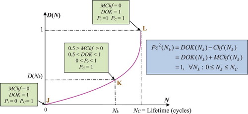
In fact, at the beginning (N_k = 0) (point J) the system is intact, then the system failure probability P_r = 0, the chaotic factor in our prediction is zero (MChf = 0) since no chaos exists yet, and our knowledge of the undamaged and unharmed system is certain and complete (DOK = 1); therefore,

If N_k = N_C (point L) the system is completely damaged, then RUL(N_C) = N_C − N_C = 0 and hence the system failure probability is one (P_r = 1). At this point, failure occurs. Hence, our knowledge of the completely worn-out system is certain (DOK = 1) and chaos has finished its harmful task so it is no more applicable (MChf = 0).

If 0 < N_k < N_C (point K, where J < K < L), the occurrence probability of this instant and the prediction probability of D and RUL are both less than one and uncertain in (0 < P_r < 1). This is the consequence of non-zero chaotic factors affecting the system (MChf > 0). The DOK of the system subject to chaos is hence imperfect and is accordingly less than 1 in (0.5 < DOK < 1).

Additionally, by applying here the CPP paradigm, we can therefore determine at any instant N_k () and at any point inclusively and between J and L, the system D and RUL with certainty in the set since in we have Pc = 1 always.

Furthermore, we can define two complementary events and with their respective probabilities by Then, let the probability in terms of the cycle number N_k be equal to (13) where is the classical cumulative probability distribution function (CDF) of the random variable N.

Since ; therefore, at a load cycle N = N_k we have (14)

Moreover, let us define two particular instants:

• N = N₀ = 0 which is assumed to be the initial time of functioning (system raw state) corresponding to D = D₀.

• And, N = N_C  is the failure instant (system wear-out state) corresponding to the degradation D = D_C = 1.

Consequently, the boundary conditions are the following:

• For N = N₀ = 0, we have D = D₀ ≈ 0 (the initial damage that may be nearly zero) and

• For N = N_C, we have D = D_C = 1 and .

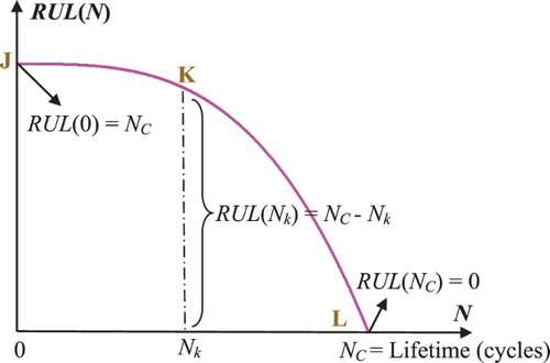
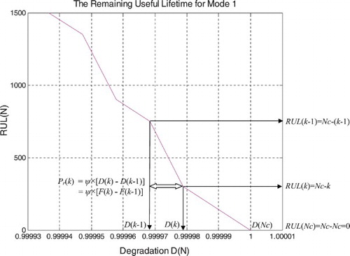
We note also that, since F(N_k) is defined as a cumulative probability function, F(N_k) is a non-decreasing function that varies between 0 and 1. In addition, since RUL(N_k) = N_C − N_k and N_k is always increasing , RUL(N_k) is a non-increasing RUL function (Figure 14).

Figure 14. The prognostic of RUL.

5.2. The new prognostic model (Beden, Abdullah, & Ariffin, 2009; Bidabad, 1992; Christensen, 2007; Cox, 1955; Fagin, Halpern, & Megiddo, 1990; Guan, Jha, & Liu, 2010; Huang, 2012; Husin, Rahman, Kadirgama, Noor, & Bakar, 2010; Ognjanović, Marković, Rašković, Doder, & Perović, 2012; Sankavaram et al., 2009; Stepić & Ognjanović, 2014; Weingarten, 2002; Xiang & Liu, 2010; Youssef, 1994)

Let us present now the basic assumption of the new prognostic model. We consider first the CDF F(N) of the random cycle number variable N as being equal to the degradation function itself, that means: (15) We note that we are dealing here with discrete random functions depending on the discrete random number of load cycles N.

This basic assumption is plausible since:

1. Both F and D are non-decreasing functions.

2. Both are cumulative functions starting from 0 and ending with 1.

3. Both functions are without measure units: F is an indicator quantifying chance and randomness, as well as D which is an indicator quantifying degradation and system damage.

Then, we assume that the real system failure probability at the instant is equal to (Figures 15 and 16) (16) where

• is the number of load cycles;

• N₀ = 0 is the initial number of cycles at the simulation beginning. It corresponds to a degradation D = D(N₀) = D₀ which is generally considered to be nearly equal to 0. Hence, since F(N_k) = D(N_k), F(N₀) = D(N₀) ≈ 0, but F(N₀) will be considered throughout this paper as being equal to zero;

• N₁ is the first load cycle;

• N_k is the kth load cycle;

• N_C is the number of cycles till system failure = the critical number of load cycles. It corresponds to D = D_C = 1. It follows directly that F(N_C) = D_C = 1.

• is the simulation magnifying factor that does not depend on the road profile. It is 14,000 for the three modes of roads (mode 1 = severe road conditions, mode 2 = fair road conditions, and mode 3 = good road conditions).

Figure 15. P_r, degradation, and the CDF step function.

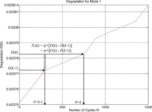
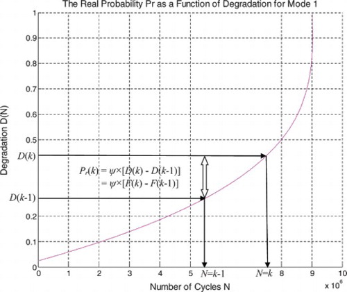
Figure 16. P_r as a function of Degradation D(N).

Thus, initially we have Moreover, (17) where is the usual PDF. Knowing that, from classical probability theory, we have always: Therefore, we can deduce that (18) This result is reasonable since is here a PDF (Figure 17).

Figure 17. Degradation and P_r.

We can observe that D(N) = F(N) is a discrete CDF where the amount of the jump is ; therefore, is a function of degradation and damage evolution (Figures 15 and 16). And we can realise from the previous calculations that is a PDF. Consequently, we can understand now that measures the probability of the system failure or degradation. Accordingly, what we have done here is that we have linked probability theory to degradation measure.

Notice that and

• If

• if .

This, since the degradation is very flat near 0 and starts increasing with N, becoming very acute at N = N_C; hence, near N_C, P_r is the greatest and is equal to 1 (Figures 16 and 17).

Furthermore, we have And This implies that (Figure 18) (19)

Figure 18. P_r, D, and RUL.

5.3. Analysis and extreme chaotic and random conditions

Although the analytic nonlinear prognostic laws are deterministic and very well known in Abou Jaoude & El-Tawil (2013a) but there are general parameters that can be random and chaotic (such as temperature, humidity, geometry dimensions, material nature, water action, soil action, applied load location, and body shape). Additionally, many variables in the equation (9) of degradation which are considered as deterministic can also have a stochastic behaviour, such as the initial crack length (potentially existing from the manufacturing process) and the applied load magnitude (due to the driving on roads of different profile conditions). All those random factors, represented in the model by their mean values, affect the system and make its degradation function deviate from its calculated trajectory predefined by these deterministic laws. An updated follow-up of the degradation behaviour with time or cycle number, and which is subject to chaotic and non-chaotic effects, is done by due to its definition that evaluates the jumps in D. In fact, chaos modifies and affects all the environment and system parameters included in the degradation equation (Equation (9)). Consequently, chaos total effect on the suspension contributes to shape the degradation curve D and is materialised by and counted in the system failure probability . Actually, quantifies the resultant of all the deterministic (non-random) and nondeterministic (random) factors and parameters which are included in the equation of D, which influence the system, and which determine the consequent final degradation curve. Accordingly, an accentuated effect of chaos on the system can lead to a bigger (or smaller) jump in the degradation trajectory and hence to a greater (or smaller) probability of failure . If for example, due to extreme deterministic causes and random factors, D jumps directly from to 1, then RUL goes straight from N_C to 0 and consequently jumps instantly from 0 to 1: where N goes directly from 0 to N_C.

In the ideal extreme case, if the system never deteriorates (no loads or stresses) and with zero chaotic causes and random factors, then the resultant of all the deterministic and nondeterministic effects is null (like in the system idle state). Consequently, the system stays indefinitely at and RUL remains equal to N_C. So accordingly the jump in D is always 0. Therefore, ideally, the probability of failure stays 0: where .

Figure 15 shows the real failure probability P_r(N) as a function of the random suspension degradation step CDF in terms of the number of load cycles N for mode 1 of roads.

Figure 16 shows the real failure probability P_r(N) as a function of the random suspension degradation in terms of the number of load cycles N for mode 1 of roads.

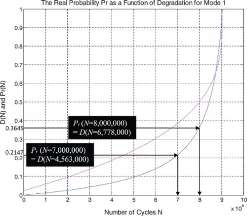
Figure 17 shows the real failure probability P_r(N) and the random suspension degradation D(N) as functions of the number of load cycles N for mode 1 of roads.

Figure 18 shows the real failure probability P_r(N) as a function of the random suspension degradation D(N) and the random suspension RUL(N) in terms of the number of load cycles N for mode 1 of roads.

5.4. The evaluation of the new paradigm parameters

We can infer from what has been elaborated previously the following: (20) (21) (22) (23)

The DOK: (24) The chaotic factor: (25)

Chf is null when P_r(N_k) = P_r(0) = 0 (point J) and when P_r(N_k) = P_r(N_C) = 1 (point L) (Figures 13 and 14).

The magnitude of the chaotic factor: (26) MChf is null when P_r(N_k) = P_r(0) = 0 (point J) and when P_r(N_k) = P_r(N_C) = 1 (point L) (Figures 13 and 14).

At any instant , the probability expressed in the complex set is the following: (27) then Pc(N_k) = P_r(N_k) + P_m(N_k)/i = P_r(N_k) + [1 − Pr(N_k)] = 1 always.

Hence, the prediction of D(N_k) and RUL(N_k) of the system in the set is permanently certain.

Let us consider thereafter the suspension system under its three road modes to simulate the cumulative distribution function F(N_k) = D(N_k) and to draw, to visualise, as well as to quantify all the CPP and prognostic parameters.

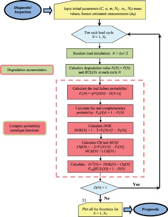
5.5. Flowchart of the complex probability nonlinear prognostic model

The following flowchart summarises all the procedures of the proposed complex probability prognostic model:

6. Simulation of the new paradigm

In this section, I will do the simulation of the novel prognostic model for the three modes of roads and load cycles. Note that all the numerical values found in the paradigm functions analysis for the three modes of roads were computed using the MATLAB version 2016 software.

6.1. The parameters analysis in the suspension prognostic for mode 1

I rescaled RUL = [0; 9,047,700] to [0; 1] in order to fit and represent it with all the CPP parameters and D which vary in [0; 1] on the same graph while having all of them as functions of the number of cycles N = [0; 9,047,700].

We notice from Figures 19–24 that the DOK is maximum (DOK = 1) when MChf is minimum (MChf = 0) (points J and L) and that means when the MChf decreases our certain knowledge (DOK) in increases.

Figure 19. Suspension degradation under nonlinear damage law for severe mode of road excitation.

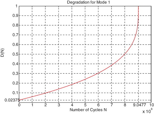
Figure 20. Suspension RUL as a function of degradation for severe mode of road excitation.

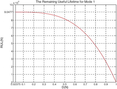
Figure 21. Degradation and CPP parameters for mode 1.

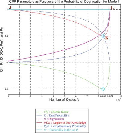
Figure 22. Degradation and CPP parameters with MChf for mode 1.

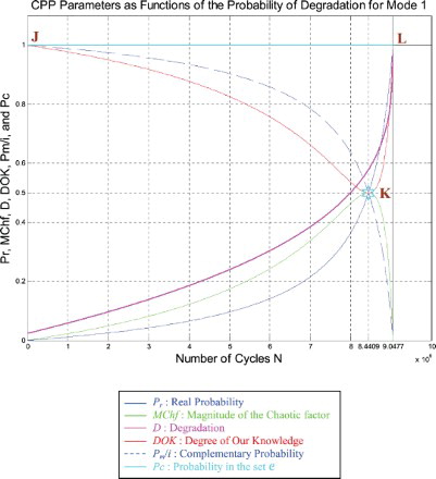
Figure 23. Degradation, rescaled RUL, and CPP parameters for mode 1.

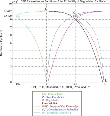
Figure 24. Degradation, rescaled RUL, and CPP parameters with MChf for mode 1.

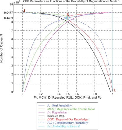
At the beginning (point J) P_r(N = N₀ = 0) = 0, the system is intact (nearly zero damage: D = D₀ = 0.02375 ≈ 0) and has zero chaotic factor (Chf(0) = MChf(0) = 0) before any usage, where at this instant (cycles number) DOK(0) = 1, RUL(0) = N_C − 0 = N_C = 9,047,700 cycles = N_C/1, and Rescaled [RUL(0)] = 0.97625. We have here the probability of the system collapse P_r(0) is 0; hence, this is the system raw state. At this point P_m/i(0) = 1, thus Pc(0) = P_r(0) + P_m/i(0) = 0 + 1 = 1 and Pc²(0) = DOK(0) + MChf(0) = 1 + 0 = 1 • Pc(0) = 1. Moreover, the complex random vector Z(0) = P_r(0) + P_m(0) = 0 + 1i = i • , just as predicted by the theory.

Afterwards N starts to increase (N > 0), then RUL(N) = N_C − N with , keeping constantly Pc(N) = P_r(N) + P_m/i(N) = 1 and Pc²(N) = DOK(N) + MChf(N) = 1 • Pc(N) = 1, therefore, MChf starts to increase also during the system functioning due to the environment and intrinsic conditions, thus leading to a decrease in DOK.

If N = N_C/2 = 9,047,700/2 = 4,523,850 cycles = half-life of the suspension system, then RUL = N_C − N_C/2 = 4,523,850 cycles = N_C/2, Rescaled (RUL) = 0.7875, D = 0.2125, DOK = 0.8528, Chf = −0.1472, MChf = 0.1472, P_r = 0.0800, P_m/i = 0.9200, with Pc = P_r + P_m/i = 0.0800 + 0.9200 = 1 and Pc² = DOK + MChf = 0.8528 + 0.1472 = 1 • Pc = 1. Moreover, the complex probability vector Z = P_r + P_m = 0.0800 + 0.9200i• , just as predicted by CPP.

If D = 0.5, then N = 7,996,000 cycles, RUL = N_C − N = 1,051,700 cycles ≈ N_C/8.603, Rescaled(RUL) = 0.5, DOK = 0.5373, Chf = −0.4627, MChf = 0.4627, P_r = 0.3635, P_m/i = 0.6365, with Pc = P_r + P_m/i = 0.3635 + 0.6365 = 1 and Pc² = DOK + MChf = 0.5373 + 0.4627 = 1 • Pc = 1. Moreover, Z = P_r + P_m = 0.3635 + 0.6365i • . At this point, both the rescaled RUL and D intersect. We can see that with the increase of N and a subsequent decrease of RUL, the probability of failure P_r increases also. Furthermore, notice in Figure 24 the complete symmetry at the vertical axis D = 1/2 = degradation half-way to complete damage.

If N = 8,440,900 cycles (point K) both DOK (minimum) and MChf (maximum) reach 0.5 where RUL(N) = N_C − N = 9,047,700 − 8,440,900 = 606,800 cycles ≈ N_C/14.911, Rescaled (RUL) = 0.4206, D = 0.5794, P_r = 0.5, P_m/i = 0.5, and Chf = −0.5, with Pc = P_r + P_m/i = 0.5 + 0.5 = 1 and Pc² = DOK + MChf = 0.5 + 0.5 = 1 • Pc = 1, as always. Moreover, Z = P_r + P_m = 0.5 + 0.5i • , just as expected. Thus, all the CPP parameters will intersect at point K. We have here the maximum of chaos and the minimum of the system knowledge; therefore, the probability of the system crash is P_r = 1/2 = probability half-way to complete damage.

If D = 0.9, then N = 9,015,000 cycles, RUL = N_C − N = 32,700 cycles ≈ N_C/276.688, Rescaled(RUL) = 0.1, DOK = 0.9007, Chf = −0.0993, MChf = 0.0993, P_r = 0.9476, P_m/i = 0.05240, Pc = P_r + P_m/i = 0.9476 + 0.05240 = 1 and Pc² = DOK + MChf = 0.9007 + 0.0993 = 1 • Pc = 1. Moreover, Z = P_r + P_m = 0.9476 + 0.05240i • . Here, since D = 0.9 which is very close to 1, the failure probability P_r is very near to 1 as we will reach total damage very soon.

With the increase of the time of functioning, N reaches at the end N_C, MChf and Chf return to zero since chaos has finished its harmful task so it is no more applicable, DOK returns to 1 where we reach total damage (D = 1) at N = N_C = 9,047,700 cycles and hence the breakdown of the system (point L). At this last point, failure here is certain, this is the system wear-out state; therefore, P_r = 1, P_m/i = 0, RUL(N) = N_C − N = N_C − N_C = 0, Rescaled (RUL) = 0, with Pc = P_r + P_m/i = 1 + 0 = 1 and Pc² = DOK + MChf = 1 + 0 = 1 • Pc = 1. Thus, the logical consequence of the value of DOK(N_C) = 1 follows since our knowledge of the entirely deteriorated system is total and complete, just like DOK(N₀) = 1 where our knowledge of the entirely unharmed system is total and complete also. Moreover, Z = P_r + P_m = 1 + 0i = 1 • the square of the norm of the vector Z is , just as predicted by CPP.

We note that the same logic and analysis concerning the degradation, the RUL, as well as all the CPP parameters apply for all the three modes of roads. In fact, the same consequences and results will be reached for the other two road modes, just like mode 1.

6.1.1. The complex probability cubes for mode 1

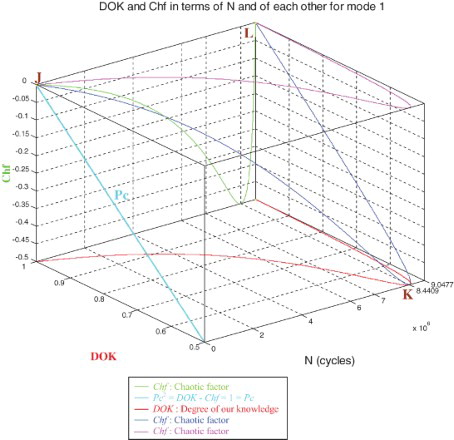
In the first cube (Figure 25), we can see the simulation of DOK and Chf as functions of each other and of the cycles number N for mode 1 of roads. The line in cyan is the projection of Pc²(N) = DOK(N) − Chf(N) = 1 = Pc(N) on the plane N = 0. This line starts at point J (DOK = 1, Chf = 0) when N = 0 cycles, reaches the point (DOK = 0.5, Chf = −0.5) when N = 8,440,900 cycles, and returns at the end to J (DOK = 1, Chf = 0) when N = N_C = 9,047,700 cycles. The other curves are the graphs of DOK(N) (red) and Chf(N) (green, blue, pink) in different planes. Notice that they all have a minimum at point K (DOK = 0.5, Chf = −0.5, N = 8,440,900 cycles). Point L corresponds to (DOK = 1, Chf = 0, N = N_C = 9,047,700 cycles). The three points J, K, and L are the same as in Figures 21–24.

Figure 25. DOK and Chf in terms of N and of each other for mode 1.

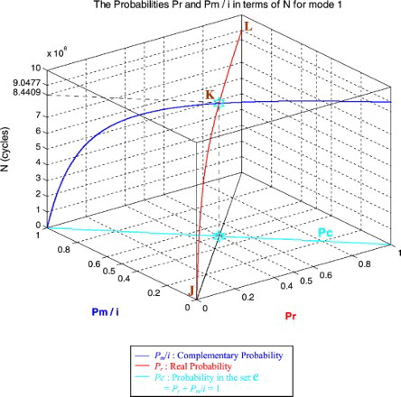
In the second cube (Figure 26), we can notice the simulation of the failure probability P_r(N) and its complementary real probability P_m/i(N) in terms of the cycles number N for mode 1 of roads. The line in cyan is the projection of Pc²(N) = P_r(N) + P_m/i(N) = 1 = Pc(N) on the plane N = 0. This line starts at the point (P_r = 0, P_m/i = 1) and ends at the point (P_r = 1, P_m/i = 0). The red curve represents P_r(N) in the plane P_r(N) = P_m/i(N). This curve starts at point J (P_r = 0, P_m/i = 1, N = 0 cycles), reaches point K (P_r = 0.5, P_m/i = 0.5, N = 8,440,900 cycles), and gets at the end to L (P_r = 1, P_m/i = 0, N = N_C = 9,047,700 cycles). The blue curve represents P_m/i(N) in the plane P_r(N) + P_m/i(N) = 1. Notice the importance of point K which is the intersection of the red and blue curves at N = 8,440,900 cycles and when P_r(N) = P_m/i(N) = 0.5. The three points J, K, and L are the same as in Figures 21–24.

Figure 26. P_r and P_m/i in terms of N and of each other for mode 1.

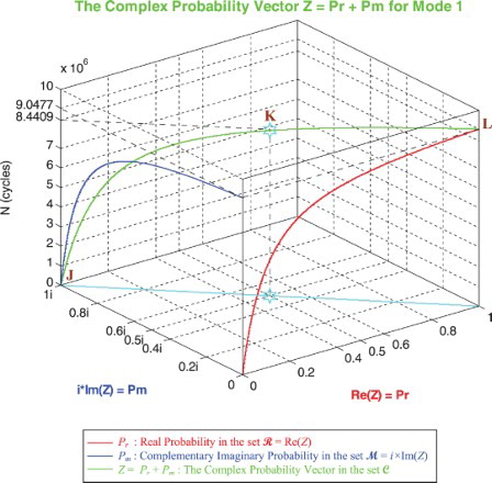
In the third cube (Figure 27), we can notice the simulation of the complex random vector Z(N) in as a function of the real failure probability P_r(N) = Re(Z) in and of its complementary imaginary probability P_m(N) = i × Im(Z) in , and this in terms of the cycles number N for mode 1 of roads. The red curve represents P_r(N) in the plane P_m(N) = 0 and the blue curve represents P_m(N) in the plane P_r(N) = 0. The green curve represents the complex probability vector Z(N) = P_r(N) + P_m(N) = Re(Z) + i × Im(Z) in the plane P_r(N) = iP_m(N) + 1. The curve of Z(N) starts at point J (P_r = 0, P_m = i, N = 0 cycles) and ends at point L (P_r = 1, P_m = 0, N = N_C = 9,047,700 cycles). The line in cyan is P_r(0) = iP_m(0) + 1 and it is the projection of the Z(N) curve on the complex probability plane whose equation is N = 0 cycles. This projected line starts at point J (P_r = 0, P_m = i, N = 0 cycles) and ends at the point (P_r = 1, P_m = 0, N = 0 cycles). Notice the importance of point K corresponding to N = 8,440,900 cycles and when P_r = 0.5 and P_m = 0.5i. The three points J, K, and L are the same as in Figures 21–24. Note that similar cubes can be drawn for modes 2 and 3 with their corresponding N_C and points J, K, and L.

Figure 27. The complex probability vector Z in terms of N for mode 1.

6.2. The parameters analysis in the suspension prognostic for mode 2

Just like for mode 1 simulations, I rescaled RUL = [0; 12,063,800] to [0; 1] in order to fit and represent it with all the CPP parameters and D which vary in [0; 1] on the same graph while having all of them as functions of the number of cycles N = [0; 12,063,800].

We note from Figures 28–33 that the DOK is maximum (DOK = 1) when MChf is minimum (MChf = 0) (points J and L) and that means when the MChf decreases our certain knowledge (DOK) in increases.

At the beginning (point J) P_r(N = N₀ = 0) = 0, the system is intact (nearly zero damage: D = D₀ = 0.02375 ≈ 0) and has zero chaotic factor (Chf(0) = MChf(0) = 0) before any usage. At this instant (cycles number) DOK(0) = 1 and RUL(0) = N_C − 0 = N_C = 12,063,800 cycles = N_C/1, Rescaled[RUL(0)] = 0.97625. Here P_m/i(0) = 1, with Pc(0) = P_r(0) + P_m/i(0) = 0 + 1 = 1 and Pc²(0) = DOK(0) + MChf(0) = 1 + 0 = 1 • Pc(0) = 1. Moreover, the complex random vector Z(0) = P_r(0) + P_m(0) = 0 + 1i = i • , just as predicted by the theory.

Afterward N starts to increase (N > 0), then RUL(N) = N_C − N with , keeping constantly Pc(N) = P_r(N) + P_m/i(N) = 1 and Pc²(N) = DOK(N) + MChf(N) = 1 • Pc(N) = 1, therefore MChf starts to increase also during the system functioning due to the environment and intrinsic conditions, thus leading to a decrease in DOK.

If N = N_C/2 = 12,063,800/2 = 6,031,900 cycles = half-life of the suspension system, then RUL = N_C − N_C/2 = 12,063,800 − 6,031,900 = 6,031,900 cycles = N_C/2, Rescaled (RUL) = 0.7875, D = 0.2125, DOK = 0.8528, Chf = −0.1472, MChf = 0.1472, P_r = 0.0800, P_m/i = 0.9200, with Pc = P_r + P_m/i = 0.0800 + 0.9200 = 1 and Pc² = DOK + MChf = 0.8528 + 0.1472 = 1 • Pc = 1. Moreover, the complex probability vector Z = P_r + P_m = 0.0800 + 0.9200i • , just as predicted.

If D = 0.5, then N = 10,660,000 cycles, RUL = N_C− N = 1,403,800 cycles ≈ N_C/8.594, Rescaled(RUL) = 0.5, DOK = 0.5369, Chf = −0.4631, MChf = 0.4631, P_r = 0.3641, P_m/i = 0.6359, with Pc = P_r + P_m/i = 0.3641 + 0.6359 = 1 and Pc² = DOK + MChf = 0.5369 + 0.4631 = 1 • Pc = 1. Moreover, Z = P_r + P_m = 0.3641 + 0.6359i • . At this point, both the rescaled RUL and D intersect. We can see that with the increase of N and a subsequent decrease of RUL, the probability of failure P_r increases also. Furthermore, notice in Figure 33 the complete symmetry at the vertical axis D = 1/2 = degradation half-way to complete damage.

If N = 11,255,000 cycles (point K) both DOK (minimum) and MChf (maximum) reach 0.5 where RUL(N) = N_C − N = 12,063,800 − 11,255,000 = 808,800 cycles ≈ N_C/14.916, Rescaled (RUL) = 0.4213, D = 0.5787, P_r = 0.5, P_m/i = 0.5, and Chf = −0.5, with Pc = P_r + P_m/i = 0.5 + 0.5 = 1, and Pc² = DOK + MChf = 0.5 + 0.5 = 1 • Pc = 1, as always. Moreover, Z = P_r + P_m = 0.5 + 0.5i • , just as expected. Thus, all the CPP parameters will intersect at point K. We have here the maximum of chaos and the minimum of the system certain knowledge; therefore, the probability of the system crash is P_r = 1/2 = probability half-way to complete damage. We note that relatively to mode 1 (severe road conditions), point K in Figures 30–33 is no more at (8,440,900; 0.5) but shifted to the right and is now at (11,255,000; 0.5) since the degradation curve for mode 2 (fair road conditions) is naturally different. Hence, DOK, Chf, and MChf are more skewed to the left relatively to mode 1.

If D = 0.9, then N = 12,040,000 cycles, RUL = N_C − N = 23,800 cycles ≈ N_C/506.882, Rescaled(RUL) = 0.1, DOK = 0.9326, Chf = −0.0674, MChf = 0.0674, P_r = 0.9651, P_m/i = 0.0349, Pc = P_r + P_m/i = 0.9651 + 0.0349 = 1 and Pc² = DOK + MChf = 0.9326 + 0.0674 = 1 • Pc = 1. Moreover, Z = P_r + P_m = 0.9651 + 0.0349i • . Here, since D = 0.9 which is very close to 1, the failure probability P_r is very near to 1 as we will reach total damage very soon.

With the increase of the time of functioning, N reaches at the end N_C, MChf and Chf return to zero since chaos has finished its harmful task so it is no more applicable, DOK returns to 1 where we reach total damage (D = 1) at N = N_C = 12,063,800 cycles and hence the breakdown of the system (point L). At this last point, failure here is certain, this is the system wear-out state; therefore, P_r = 1, P_m/i = 0, RUL(N) = N_C − N = N_C − N_C = 0, Rescaled (RUL) = 0, with Pc = P_r + P_m/i = 1 + 0 = 1 and Pc² = DOK + MChf = 1 + 0 = 1 • Pc = 1. Thus, the logical consequence of the value of DOK(N_C) = 1 follows since our knowledge of the entirely deteriorated system is total and complete, just like DOK(N₀) = 1 where our knowledge of the entirely unharmed system is total and complete also. Moreover, Z = P_r + P_m = 1 + 0i = 1 • the square of the norm of the vector Z is , just as predicted by CPP.

We note that the same logic and analysis for mode 1 of roads are applied to mode 2 of roads concerning the degradation, the RUL, as well as all the CPP parameters. In fact, the same consequences and results will be reached for road mode 3, just like the first two modes.

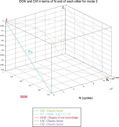
6.2.1. The complex probability cubes for mode 2

In the first cube (Figure 34), we can see the simulation of DOK and Chf as functions of each other and of the cycles number N for mode 2 of roads. The line in cyan is the projection of Pc²(N) = DOK(N) − Chf(N) = 1 = Pc(N) on the plane N = 0. This line starts at point J (DOK = 1, Chf = 0) when N = 0 cycles, reaches the point (DOK = 0.5, Chf = −0.5) when N = 11,255,000 cycles, and returns at the end to J (DOK = 1, Chf = 0) when N = N_C = 12,063,800 cycles. The other curves are the graphs of DOK(N) (red) and Chf(N) (green, blue, pink) in different planes. Notice that they all have a minimum at point K (DOK = 0.5, Chf = −0.5, N = 11,255,000 cycles). Point L corresponds to (DOK = 1, Chf = 0, N = N_C = 12,063,800 cycles). The three points J, K, and L are the same as in Figures 30–33.

Figure 28. Suspension degradation under nonlinear damage law for fair mode of road excitation.

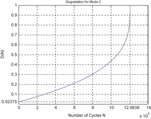
Figure 29. Suspension RUL as a function of degradation for fair mode of road excitation.

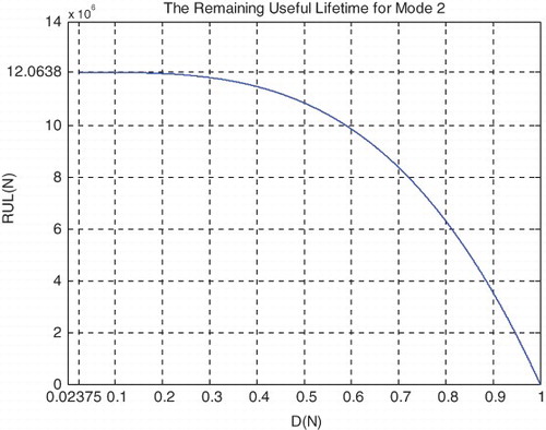
Figure 30. Degradation and CPP parameters for mode 2.

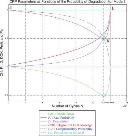
Figure 31. Degradation and CPP parameters with MChf for mode 2.

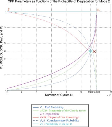
Figure 32. Degradation, rescaled RUL, and CPP parameters for mode 2.

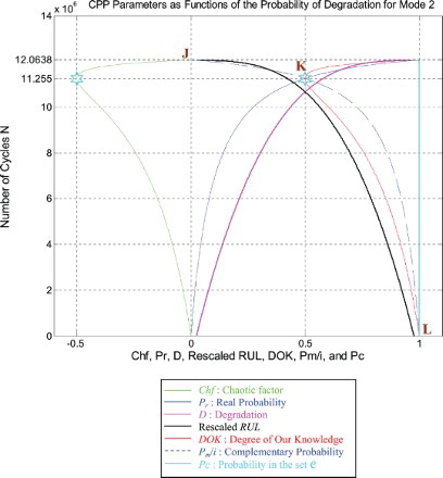
Figure 33. Degradation, rescaled RUL, and CPP parameters with MChf for mode 2.

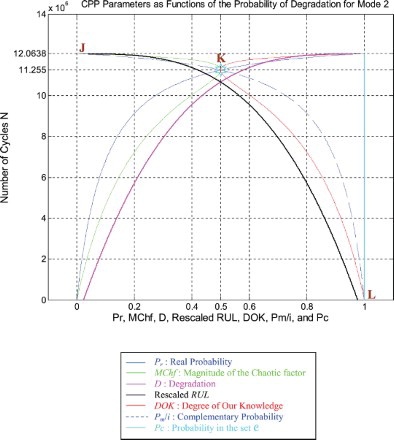
Figure 34. DOK and Chf in terms of N and of each other for mode 2.

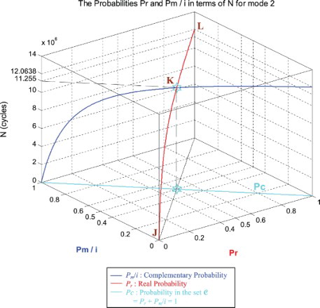
In the second cube (Figure 35), we can notice the simulation of the failure probability P_r(N) and its complementary real probability P_m/i(N) in terms of the cycles number N for mode 2 of roads. The line in cyan is the projection of Pc²(N) = P_r(N) + P_m/i(N) = 1 = Pc(N) on the plane N = 0. This line starts at the point (P_r = 0, P_m/i = 1) and ends at the point (P_r = 1, P_m/i = 0). The red curve represents P_r(N) in the plane P_r(N) = P_m/i(N). This curve starts at point J (P_r = 0, P_m/i = 1, N = 0 cycles), reaches point K (P_r = 0.5, P_m/i = 0.5, N = 11,255,000 cycles), and gets at the end to L (P_r = 1, P_m/i = 0, N = N_C = 12,063,800 cycles). The blue curve represents P_m/i(N) in the plane P_r(N) + P_m/i(N) = 1. Notice the importance of point K which is the intersection of the red and blue curves at N = 11,255,000 cycles and when P_r(N) = P_m/i(N) = 0.5. The three points J, K, and L are the same as in Figures 30–33.

Figure 35. P_r and P_m/i in terms of N and of each other for mode 2.

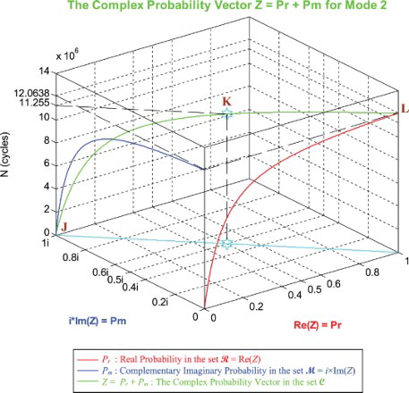
In the third cube (Figure 36), we can notice the simulation of the complex random vector Z(N) in as a function of the real failure probability P_r(N) = Re(Z) in and of its complementary imaginary probability P_m(N) = i × Im(Z) in , and this in terms of the cycles number N for mode 2 of roads. The red curve represents P_r(N) in the plane P_m(N) = 0 and the blue curve represents P_m(N) in the plane P_r(N) = 0. The green curve represents the complex probability vector Z(N) = P_r(N) + P_m(N) = Re(Z) + i × Im(Z) in the plane P_r(N) = iP_m(N) + 1. The curve of Z(N) starts at point J (P_r = 0, P_m = i, N = 0 cycles) and ends at point L (P_r = 1, P_m = 0, N = N_C = 12,063,800 cycles). The line in cyan is P_r(0) = iP_m(0) + 1 and it is the projection of the Z(N) curve on the complex probability plane whose equation is N = 0 cycles. This projected line starts at point J (P_r = 0, P_m = i, N = 0 cycles) and ends at point (P_r = 1, P_m = 0, N = 0 cycles). Notice the importance of point K corresponding to N = 11,255,000 cycles and when P_r = 0.5 and P_m = 0.5i. The three points J, K, and L are the same as in Figures 30–33. Note that similar cubes can be drawn for mode 3 with its corresponding N_C and points J, K, and L.

Figure 36. The complex probability vector Z in terms of N for mode 2.

6.3. The parameters analysis in the suspension prognostic for mode 3:

Just like for modes 1 and 2 simulations, I rescaled RUL = [0; 18,095,400] to [0; 1] in order to fit and represent it with all the CPP parameters and D which vary in [0; 1] on the same graph while having all of them as functions of the number of cycles N = [0; 18,095,400].

We note from Figures 37–42 that the DOK is maximum (DOK = 1) when MChf is minimum (MChf = 0) (points J and L) and that means when the MChf decreases our certain knowledge (DOK) in increases.

At the beginning (point J) P_r(N = N₀ = 0) = 0, the system is intact (nearly zero damage: D = D₀ = 0.02375 ≈ 0) and has zero chaotic factor (Chf(0) = MChf(0) = 0) before any usage, where at this instant (cycles number) DOK(0) = 1, RUL(0) = N_C − 0 = N_C = 18,095,400 cycles = N_C/1, and Rescaled [RUL(0)] = 0.97625. Here P_m/i(0) = 1 with Pc(0) = P_r(0) + P_m/i(0) = 0 + 1 = 1 and Pc²(0) = DOK(0) + MChf(0) = 1 + 0 = 1 • Pc(0) = 1. Moreover, the complex random vector Z(0) = P_r(0) + P_m(0) = 0 + 1i = i • , just as predicted by the theory.

Afterward N starts to increase (N > 0), then RUL(N) = N_C − N with P_r(N) = ψ × [D(N) − D(N − 1)] ≠ 0, keeping constantly Pc(N) = P_r(N) + P_m/i(N) = 1 and Pc²(N) = DOK(N) + MChf(N) = 1 • Pc(N) = 1, therefore MChf starts to increase also during the system functioning due to the environment and intrinsic conditions, thus leading to a decrease in DOK.

If N = N_C/2 = 18,095,400/2 = 9,047,700 cycles = half-life of the suspension system, then RUL = N_C − N_C/2 = 18,095,400 − 9,047,700 = 9,047,700 cycles = N_C/2, Rescaled (RUL) = 0.7874, D = 0.2126, DOK = 0.8528, Chf = −0.1472, MChf = 0.1472, P_r = 0.0800, P_m/i = 0.9200, with Pc = P_r + P_m/i = 0.0800 + 0.9200 = 1 and Pc² = DOK + MChf = 0.8528 + 0.1472 = 1 • Pc = 1. Moreover, the complex probability vector Z = P_r + P_m = 0.0800 + 0.9200i • .

If D = 0.5, then N = 15,990,000 cycles, RUL = N_C − N = 2,105,400 cycles ≈ N_C/8.595, Rescaled(RUL) = 0.5, DOK = 0.5370, Chf = −0.4630, MChf = 0.4630, P_r = 0.3639, P_m/i = 0.6361, with Pc = P_r + P_m/i = 0.3639 + 0.6361 = 1 and Pc² = DOK + MChf = 0.5370 + 0.4630 = 1 • Pc = 1. Moreover, Z = P_r + P_m = 0.3639 + 0.6361i • . At this point, both the rescaled RUL and D intersect. We can see that with the increase of N and consequently the decrease of RUL, the probability of failure P_r increases also. Furthermore, notice in Figure 42 the complete symmetry at the vertical axis D = 1/2 = degradation half-way to complete damage.

If N = 16,882,000 cycles (point K) both DOK (minimum) and MChf (maximum) reach 0.5 where RUL(N) = N_C − N = 18,095,400 − 16,882,000 = 1,213,400 cycles ≈ N_C/14.913, Rescaled (RUL) = 0.4214, D = 0.5786, P_r = 0.5, P_m/i = 0.5, and Chf = −0.5 with Pc = P_r + P_m/i = 0.5 + 0.5 = 1 and Pc² = DOK + MChf = 0.5 + 0.5 = 1 • Pc = 1, as always. Moreover, the complex probability vector Z = P_r + P_m = 0.5 + 0.5i • , just as expected. Hence, all the CPP parameters will intersect at point K. We have here the maximum of chaos and the minimum of the system knowledge; therefore, the probability of the system crash is P_r = 1/2 = probability half-way to complete damage. We note that relatively to mode 1 (severe road conditions) and mode 2 (fair road conditions), point K in Figures 39–42 is no more at (8,440,900; 0.5) or (11,255,000; 0.5) but shifted more to the right and is now at (16,882,000; 0.5) since the degradation curve for mode 3 (good road conditions) is eventually different. Hence, DOK, Chf, and MChf are more negatively skewed relatively to modes 1 and 2.

If D = 0.9, then N = 18,060,000 cycles, RUL = N_C − N = 35,400 cycles ≈ N_C/511.169, Rescaled(RUL) = 0.1, DOK = 0.9364, Chf = −0.0636, MChf = 0.0636, P_r = 0.9671, P_m/i = 0.0329, with Pc = P_r + P_m/i = 0.9671 + 0.0329 = 1 and Pc² = DOK + MChf = 0.9364 + 0.0636 = 1 • Pc = 1. Moreover, Z = P_r + P_m = 0.9671 + 0.0329i • , just as expected. Here, since D = 0.9 which is very close to 1, then the failure probability P_r is very near to 1 as we will reach total damage very soon.

With the increase of the time of functioning, N reaches at the end N_C, MChf and Chf return to zero since chaos has finished its harmful task so it is no more applicable, DOK returns to 1 where we reach total damage (D = 1) at N = N_C = 18,095,400 cycles and hence the breakdown of the system (point L). At this last point, failure here is certain, this is the system wear-out state; therefore, P_r = 1, P_m/i = 0, RUL(N) = N_C − N = N_C − N_C = 0, Rescaled (RUL) = 0, with Pc = P_r + P_m/i = 1 + 0 = 1 and Pc² = DOK + MChf = 1 + 0 = 1 • Pc = 1. Thus, the logical consequence of the value of DOK(N_C) = 1 follows since our knowledge of the entirely deteriorated system is total and complete, just like DOK(N₀) = 1 where our knowledge of the entirely unharmed system is total and complete also. Moreover, Z = P_r + P_m = 1 + 0i = 1 • the square of the norm of the vector Z is , just as predicted by CPP.

6.3.1. The complex probability cubes for mode 3

In the first cube (Figure 43), we can see the simulation of DOK and Chf as functions of each other and of the cycles number N for mode 3 of roads. The line in cyan is the projection of Pc²(N) = DOK(N) − Chf(N) = 1 = Pc(N) on the plane N = 0. This line starts at point J (DOK = 1, Chf = 0) when N = 0 cycles, reaches the point (DOK = 0.5, Chf = −0.5) when N = 16,882,000 cycles, and returns at the end to J (DOK = 1, Chf = 0) when N = N_C = 18,095,400 cycles. The other curves are the graphs of DOK(N) (red) and Chf(N) (green, blue, pink) in different planes. Notice that they all have a minimum at point K (DOK = 0.5, Chf = −0.5, N = 16,882,000 cycles). Point L corresponds to (DOK = 1, Chf = 0, N = N_C = 18,095,400 cycles). The three points J, K, and L are the same as in Figures 39–42.

In the second cube (Figure 44), we can notice the simulation of the failure probability P_r(N) and its complementary real probability P_m/i(N) in terms of the cycles number N for mode 3 of roads. The line in cyan is the projection of Pc²(N) = P_r(N) + P_m/i(N) = 1 = Pc(N) on the plane N = 0. This line starts at the point (P_r = 0, P_m/i = 1) and ends at the point (P_r = 1, P_m/i = 0). The red curve represents P_r(N) in the plane P_r(N) = P_m/i(N). This curve starts at point J (P_r = 0, P_m/i = 1, N = 0 cycles), reaches point K (P_r = 0.5, P_m/i = 0.5, N = 16,882,000 cycles), and gets at the end to L (P_r = 1, P_m/i = 0, N = N_C = 18,095,000 cycles). The blue curve represents P_m/i(N) in the plane P_r(N) + P_m/i(N) = 1. Notice the importance of point K which is the intersection of the red and blue curves at N = 16,882,000 cycles and when P_r(N) = P_m/i(N) = 0.5. The three points J, K, and L are the same as in Figures 39–42.

In the third cube (Figure 45), we can notice the simulation of the complex random vector Z(N) in as a function of the real failure probability P_r(N) = Re(Z) in and of its complementary imaginary probability P_m(N) = i × Im(Z) in , and this in terms of the cycles number N for mode 3 of roads. The red curve represents P_r(N) in the plane P_m(N) = 0 and the blue curve represents P_m(N) in the plane P_r(N) = 0. The green curve represents the complex probability vector Z(N) = P_r(N) + P_m(N) = Re(Z) + i × Im(Z) in the plane P_r(N) = iP_m(N) + 1. The curve of Z(N) starts at point J (P_r = 0, P_m = i, N = 0 cycles) and ends at point L (P_r = 1, P_m = 0, N = N_C = 18,095,000 cycles). The line in cyan is P_r(0) = iP_m(0) + 1 and it is the projection of the Z(N) curve on the complex probability plane whose equation is N = 0 cycles. This projected line starts at point J (P_r = 0, P_m = i, N = 0 cycles) and ends at the point (P_r = 1, P_m = 0, N = 0 cycles). Notice the importance of point K corresponding to N = 16,882,000 cycles and when P_r = 0.5 and P_m = 0.5i. The three points J, K, and L are the same as in Figures 39–42.

6.4. The parameters visualisation in the suspension prognostic for the three modes

Furthermore, the simulations given in Figures 46–51 recapitulate all the previous ones in Figures 19–45. They are three-in-one figures.

6.5. Simulations interpretation, final analysis, and the general prognostic equations

In this section, I will interpret all the simulations, do a final analysis, and present the novel general prognostic equations. Firstly, I linked probability theory represented by the CDF F(N) with prognostic represented by the degradation D(N) by supposing that F(N) = D(N) and I gave the justification for this assumption. In doing so, the deterministic D(N) taken from deterministic analytic nonlinear prognostic becomes a nondeterministic CDF. Thus, the discrete and deterministic variable of load cycles N becomes a discrete random variable. Therefore, the resultant of all the factors acting on the suspension which was deterministic becomes a random resultant since D(N) measures now the suspension random degradation as a function of the random cycle number N. Hence, all the exact parameters values of the D(N) equation (9) now become mean values of the random factors affecting the system and are represented by PDFs as functions of the random variable of load cycles N (refer to Section 4.4). In fact, this is the real world case where randomness is omnipresent in one form or another. What we experience and consider as a deterministic phenomenon is nothing in reality but an approximation and a simplification of an actual stochastic and chaotic experiment due to the impact of a huge number of deterministic and nondeterministic factors and forces (a lottery machine is a good example).

Consequently, an updated follow-up of the random degradation behaviour with time or cycle number, and which is subject to chaotic and non-chaotic effects, is done by the quantity due to its definition that evaluates the jumps in the stochastic degradation CDF D(N). Hence, Referring to classical probability theory, this makes the system probability of failure at N = N_k, with and , just like any PDF.

Figure 37. Suspension degradation under nonlinear damage law for good mode of road excitation.

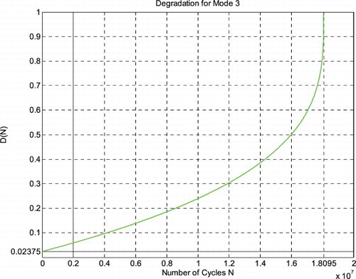
Figure 38. Suspension RUL as a function of degradation for good mode of road excitation.

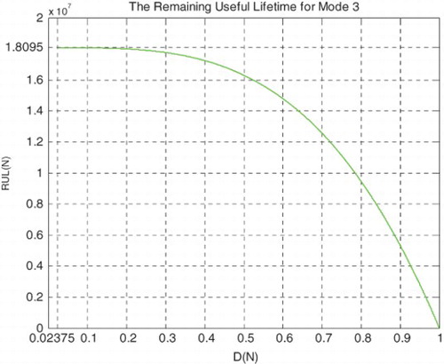
Figure 39. Degradation and CPP parameters for mode 3.

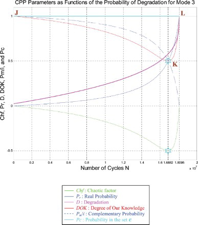
Figure 40. Degradation and CPP parameters with MChf for mode 3.

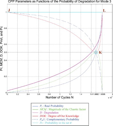
Figure 41. Degradation, rescaled RUL, and CPP parameters for mode 3.

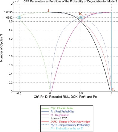
Figure 42. Degradation, rescaled RUL, and CPP parameters with MChf for mode 3.

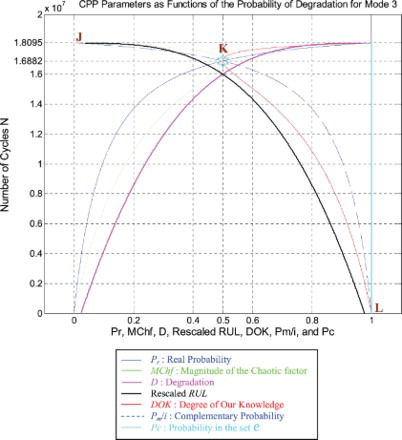
Figure 43. DOK and Chf in terms of N and of each other for mode 3.

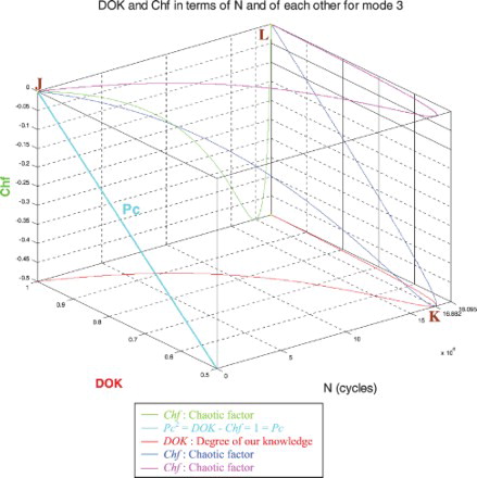
Figure 44. P_r and P_m/i in terms of N and of each other for mode 3.

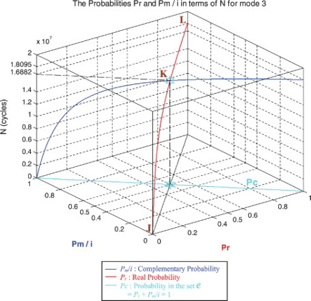
Figure 45. The complex probability vector Z in terms of N for mode 3.

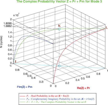
Figure 46. Suspension degradation under nonlinear damage law for the three modes of road excitation.

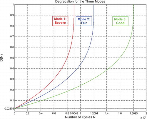
Figure 47. Suspension RUL as a function of degradation for the three modes of road excitation.

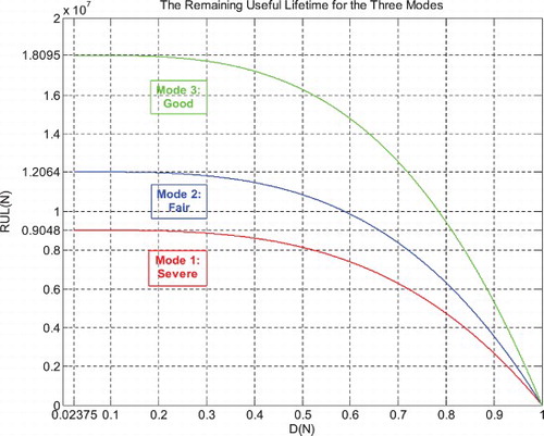
Figure 48. Degradation and CPP parameters for the three modes.

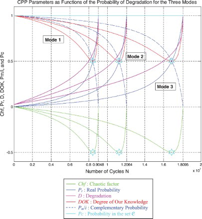
Figure 49. Degradation and CPP parameters with MChf for the three modes.

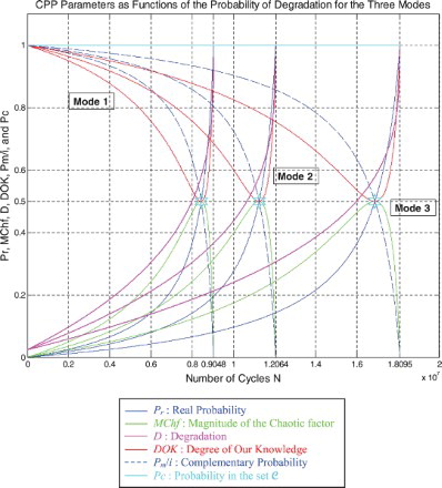
Figure 50. Degradation, rescaled RUL, and CPP parameters for the three modes.

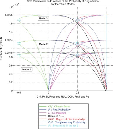
Figure 51. Degradation, rescaled RUL, and CPP parameters with MChf for the three modes.

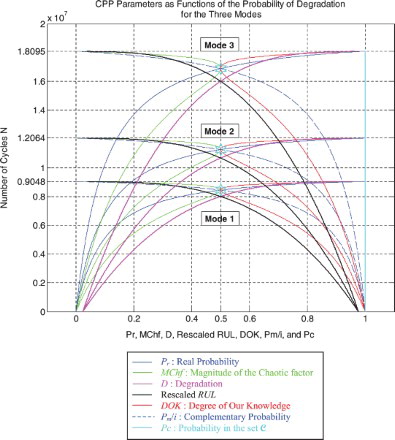
In addition, in the simulations, I have taken a constant and very small increments in N which lead to very small increments in D and hence in . So by multiplying those very small jumps in D by a simulation magnifying factor that I called and = 14,000 we get: if N tends to 0, then tends to 0, and if N tends to N_C, then tends to 1, so and as if were a CDF although mathematically speaking it is not at all. This, since is not cumulative, it is just times the probability of failure at N = N_k. Hence, in the simulations, becomes now the probability that the system failure occurs at N = N_k.

Therefore, D(N_k) = F(N_k) = P_rob(0 ≤ N ≤ N_k) =P_rob (N = 0 or N = 1 or N = 2 or … or N = N_k) = sum of all failure probabilities between 0 and N_k = probability that failure will occur somewhere between 0 and N_k. So if N_k = 0, then = probability that failure will occur at N = 0 and before. If N_k = N_C, then = sum of all failure probabilities between 0 and N_C = probability that failure will occur somewhere between 0 and N_C. If N_k > N_C, then = probability that failure will occur beyond N_C. We can see that failure probability increases with the increase of the load cycle number N_k until at the end it becomes 1 when .

Hence, if and , then: This implies that and If and , then the prognostic equation in the new model is (28) with .

In the general prognostic case, if we have the system failure PDF, then we can include it in Equation (28) and determine degradation and vice versa. Then, all the other model CPP functions (Chf, MChf, DOK, Z, P_r, P_m, P_m/i, Pc) will follow. This would be our new prognostic model general equation: (29)

Additionally, in the three road modes’ simulations, and by applying CPP to the suspension prognostic, we succeeded in the novel prognostic model to quantify in (our real laboratory) both our certain knowledge represented by DOK and chaos represented by Chf and MChf. These three CPP parameters are caused and evaluated by the resultant of all the deterministic (non-random) and nondeterministic (random) factors affecting the suspension system. Knowing that, in the new model, the factors’ resultant effect on D and RUL is concretised by the jumps in their curves and is accordingly measured and expressed in by P_r and in by P_m. As defined in CPP, is an imaginary extension of the real probability set and the complex set is the sum of both probability sets; hence, . Since P_m = i(1 − P_r), it is the complementary probability in of P_r. So if P_r is defined as the system failure probability in at the cycle number N = N_k, then P_m is the corresponding probability in the set that the system failure will not occur at the same cycle number N = N_k. Thus, P_m is the associated probability in the set of the system survival at N = N_k. Accordingly, P_m/i = 1 − P_r is the associated probability but in the set of the system survival at the same cycle number. From classical probability theory, we know that the sum in of both complementary probabilities is surely 1. This sum is nothing but P_C which is equal to P_r + P_m/i = P_r + (1 − P_r) = 1 always. The sum in of both complementary probabilities is the complex random number and vector Z which is equal to P_r + P_m = P_r + i(1 − P_r). And as it was shown and illustrated in the complex probability cubes paragraphs, we understand that Z is the sum in of the real failure probability and of the imaginary survival probability in the complex probability plane whose equation is P_r(N) = iP_m(N) + 1 for , , . What is interesting is that the square of the norm of Z which is is nothing but DOK, as it was proved in CPP and in the new model. Moreover, since MChf = −2iP_rP_m = 2P_rP_m/i, it is twice the product in of both the failure probability and the survival probability and it measures the magnitude of chaos since it is always zero or positive. All these facts are shown and proved in all the simulations.

From all the above, we can conclude that since D(N) is a CDF, the factors resultant is random, the jumps in D are the failure probabilities , then we are dealing with a random experiment, thus the natural appearance of Chf, MChf, DOK, Z, and hence Pc. So we obtain (30) (31) (32) (33) (34)

Furthermore, in the new model we have Note that, since N and D are random, RUL is also a random function of N. Thus, we have in the set : (35)

Then, we get always: everywhere.

This implies that And

Hence, we reach a new and general prognostic equation for RUL. If and , then: (36) (37)

In the ideal case, if all the factors are 100% deterministic, then we have in : the probability of failure for is 0 and is 1 for , accordingly the probability of system survival for is 1 and is 0 for , since certain failure will occur only at . So degradation is determined surely everywhere and its CDF is replaced by a deterministic function and curve. Therefore, chaos is null and hence Chf = MChf = 0 and DOK = 1 always for all . Thus, and .

Consequently, at each instant N in the novel prognostic model, the random D(N) and RUL(N) are certainly predicted in the complex set with Pc² = DOK − Chf = DOK + MChf maintained as equal to one through a continuous compensation between DOK and Chf. This compensation is from the instant N = 0 where D(N) = D₀ = 0.02375 ≈ 0 until the failure instant N_C where D(N_C) = 1. We can also understand that DOK is the measure of our certain knowledge (100% probability) about the expected event, it does not include any uncertain knowledge (with a probability less than 100%). We can see that in computing Pc² we have eliminated and subtracted in the equation above all the random factors and chaos (Chf) from our random experiment, hence no chaos exists in , it only exists (if it does) in ; therefore, this have yielded a 100% deterministic experiment and outcome in since the probability Pc is equal to 1. This is one of the advantages of extending to and hence of working in . Hence, in the novel prognostic model, our knowledge of all the parameters and indicators (P_rob, D, RUL, etc.) is always perfect, constantly complete, and totally predictable since Pc = 1 permanently, independently of any road profile or random factors.

We note finally that the same methodology, logic, and analysis for road mode 1 were applied to road modes 2 and 3 regarding the degradation, the RUL, as well as all the CPP parameters. Thus, we can consequently infer that whatever the environment and road conditions are, the results and conclusions are similar. This proves the validity of the new axioms developed and of the original prognostic model adopted.

7. Conclusion and perspectives

The high availability of technological systems, such as in aerospace, defense, petro-chemistry, and automobile, is an important goal of earlier recent developments in system design technology knowing that expensive failure can generally occur suddenly. To make the classical strategies of maintenance more efficient and to take into account the evolving product state and environment, a new analytic prognostic model was developed in my previous publications and work as a complement of existent maintenance strategies. This model was applied to vehicle suspension systems that are subject to fatigue failure under repetitive cyclic loading. Knowing that, the fatigue effects will initiate micro-cracks that can propagate suddenly and will lead to failure. This model is based on an existing damage law in fracture mechanics which is the crack propagation law of Paris–Erdogan. From a predefined threshold of degradation D_C, the RUL is estimated by this prognostic model. Damages were assumed in Abou Jaoude and El-Tawil (2013a) to be accumulated nonlinearly to take into consideration the more complex behaviour of loading and materials. The degradation model developed in this previous work is based on the accumulation of a damage measurement D after each loading cycle. When this measure reaches the predefined threshold D_C, the system is considered in wear-out state. Furthermore, the stochastic influence was included later, as well as here, to make the model more accurate and realistic. The model is applied to the automobile industry; hence, a prognostic assessment of the suspension component permits us to enhance its maintenance strategies.

Additionally, in the current paper I applied and linked the theory of EKA to the analytic and nonlinear prognostic of vehicle suspension systems. Hence, I established a tight bond between the new paradigm and degradation or the RUL. Thus, I developed the theory of ‘complex probability’ beyond the scope of my previous seven papers on this topic.

In fact, although the analytic nonlinear prognostic laws are deterministic and very well known in Abou Jaoude and El-Tawil (2013a) but there are general parameters that can be random and chaotic (such as temperature, humidity, geometry dimensions, material nature, water action, soil action, applied load location, and body shape). Additionally, many variables in Equation (9) of degradation which are considered as deterministic can also have a stochastic behaviour, such as the initial crack length (potentially existing from the manufacturing process) and the applied load magnitude (due to the driving on roads of different profile conditions). All those random factors, represented in the model by their mean values, affect the system and make its degradation function deviate from its calculated trajectory predefined by these deterministic laws. An updated follow-up of the degradation behaviour with time or cycle number, and which is subject to chaotic and non-chaotic effects, is done by the system failure probability due to its definition that evaluates the jumps in D. In fact, chaos modifies and affects all the environment and system parameters included in the degradation equation. Consequently, chaos total effect on the suspension contributes to shape the degradation curve D and is materialised by and counted in the system failure probability. Actually, quantifies the resultant of all the deterministic (non-random) and nondeterministic (random) factors and parameters which are included in the equation of D, which influence the system, and which determine the consequent final degradation curve. Accordingly, an accentuated effect of chaos on the system can lead to a bigger (or smaller) jump in the degradation trajectory and hence to a greater (or smaller) probability of failure.

Moreover, as it was proved and illustrated in the new model, when the degradation index is 0 or 1 and correspondingly the RUL is N_C or 0, then the DOK is one and the chaotic factor (Chf and MChf) is 0 since the state of the system is totally known. During the process of degradation (0 < D < 1), we have 0.5 < DOK < 1, −0.5 < Chf < 0, and 0 < MChf < 0.5. Notice that during this whole process, we have always Pc² = DOK − Chf = DOK + MChf = 1, that means that the phenomenon which seems to be random and stochastic in is now deterministic and certain in , and this after adding to the contributions of and hence after subtracting the chaotic factor from the DOK. Furthermore, I have determined the probabilities of the system failure and of survival corresponding to each instant N, as well as the probability of RUL after N load cycles, which are all functions of the random degradation jump. Therefore, at each cycle N, D(N) and RUL(N) are surely predicted in the complex set with Pc maintained as equal to 1. Furthermore, using all these illustrated graphs and simulations throughout the whole paper, we can visualise and quantify both the system chaos (Chf and MChf) and the certain knowledge (DOK and Pc) of the suspension system. This is certainly very interesting and fruitful and shows once again the benefits of extending Kolmogorov's axioms and thus the originality and usefulness of this new field in applied mathematics and prognostic that can be called verily: ‘the complex probability paradigm’.

As a prospective and future work, it is planned to develop more the novel proposed prognostic paradigm and to apply it to a wide set of dynamic systems such as onshore and offshore pipelines.

Disclosure statement

No potential conflict of interest was reported by the authors.

References

- Abou Jaoude, A. (2004). Applied mathematics: Numerical methods and algorithms for applied mathematicians (Ph.D. thesis). Bircham International University. Retrieved from http://www.bircham.edu
- Abou Jaoude, A. (2005). Computer science: Computer simulation of Monte Carlo methods and random phenomena (Ph.D. thesis). Bircham International University. Retrieved from http://www.bircham.edu
- Abou Jaoude, A. (2007). Applied statistics and probability: Analysis and algorithms for the statistical and stochastic paradigm (Ph.D. thesis). Bircham International University. Retrieved from http://www.bircham.edu
- Abou Jaoude, A. (2012). Advanced analytical model for the prognostic of industrial systems subject to fatigue (Ph.D. thesis). Aix-Marseille Université and the Lebanese University, defended on December 7.
- Abou Jaoude, A. (2013a). Automatic control and prognostic (chap. 3, pp. 115–152). Saarbrucken: Scholars’ Press.
- Abou Jaoude, A. (2013b). The complex statistics paradigm and the law of large numbers. Journal of Mathematics and Statistics, 9(4), 289–304. doi: 10.3844/jmssp.2013.289.304
- Abou Jaoude, A. (2013c). The theory of complex probability and the first order reliability method. Journal of Mathematics and Statistics, 9(4), 310–324. doi: 10.3844/jmssp.2013.310.324
- Abou Jaoude, A. (2014). Complex probability theory and prognostic. Journal of Mathematics and Statistics, 10(1), 1–24. doi: 10.3844/jmssp.2014.1.24
- Abou Jaoude, A. (2015a). Analytic and linear prognostic model for a vehicle suspension system subject to fatigue. Systems Science & Control Engineering, 3(1), 81–98. doi: 10.1080/21642583.2014.987359
- Abou Jaoude, A. (2015b). The paradigm of complex probability and the Brownian motion. Systems Science and Control Engineering, 3(1), 478–503. doi: 10.1080/21642583.2015.1108885
- Abou Jaoude, A. (2015c). The complex probability paradigm and analytic linear prognostic for vehicle suspension systems. American Journal of Engineering and Applied Sciences, 8(1), 147–175. doi: 10.3844/ajeassp.2015.147.175
- Abou Jaoude, A. (2016). The paradigm of complex probability and Chebyshev’s inequality. Systems Science and Control Engineering, 4(1), 99–137. doi: 10.1080/21642583.2016.1185044
- Abou Jaoude, A., & El-Tawil, K. (2013a). Analytic and nonlinear prognostic for vehicle suspension systems. American Journal of Engineering and Applied Sciences, 6(1), 42–56. doi: 10.3844/ajeassp.2013.42.56
- Abou Jaoude, A., & El-Tawil, K. (2013b). Stochastic prognostic paradigm for petrochemical pipelines subject to fatigue. American Journal of Engineering and Applied Sciences, 6(2), 145–160. doi: 10.3844/ajeassp.2013.145.160
- Abou Jaoude, A., El-Tawil, K., & Kadry, S. (2010). Prediction in complex dimension using Kolmogorov’s set of axioms. Journal of Mathematics and Statistics, 6(2), 116–124. doi: 10.3844/jmssp.2010.116.124
- Abou Jaoude, A., El-Tawil, K., Kadry, S., Noura, H., & Ouladsine, M. (2010). Analytic prognostic model for a dynamic system. International Review of Automatic Control, 3(6), 568–577.
- Abou Jaoude, A., El-Tawil, K., Kadry, S., Noura, H., & Ouladsine, M. (2011). Prognostic model for buried tubes. Paper presented at the International Conference on Advanced Research and Applications in Mechanical Engineering (ICARAME’11), Notre Dame University, Louaizé.
- Abou Jaoude, A., Kadry, S., El-Tawil, K., Noura, H., & Ouladsine, M. (2011). Analytic prognostic for petrochemical pipelines. Journal of Mechanical Engineering Research, 3(3), 64–74.
- Abou Jaoude, A., Noura, H., El-Tawil, K., Kadry, S., & Ouladsine, M. (2012a). Lifetime analytic prognostic for petrochemical pipes subject to fatigue. Paper presented at SAFEPROCESS, Eighth IFAC Symposium on Fault Detection, Supervision and Safety of Technical Processes, Mexico City.
- Abou Jaoude, A., Noura, H., El-Tawil, K., Kadry, S., & Ouladsine, M. (2012b). Analytic prognostic model for stochastic fatigue of petrochemical pipelines. Paper presented at Australian Control Conference (AUCC 2012), Sydney.
- Abrams, W. A brief history of probability (2nd moment). Retrieved May 23, 2008, from http://www.secondmoment.org/articles/probability.php.
- Aczel, A. (2000). God‘s equation. New York: Dell.
- Balibar, F. (2002). Albert Einstein: Physique, philosophie, politique (1st ed.). Paris: Le Seuil.
- Barrow, J. (1992). Pi in the sky. London: Oxford University Press.
- Beden, S. M., Abdullah, S., & Ariffin, A. K. (2009). Review of fatigue crack propagation models for metallic components. European Journal of Scientific Research, 28(3), 364–397.
- Bell, E. T. (1992). The development of mathematics. New York: Dover.
- Benton, W. (1966a). Probability, encyclopedia Britannica (Vol. 18). Chicago, IL: Encyclopedia Britannica.
- Benton, W. (1966b). Mathematical probability, encyclopedia Britannica (Vol. 18). Chicago, IL: Encyclopedia Britannica.
- Bidabad, B. (1992). Complex probability and Markov stochastic processes. Paper presented at the Proceedings of First Iranian Statistics Conference, Tehran. Isfahan University of Technology.
- Bogdanov, I., & Bogdanov, G. (2009). Au commencement du temps. Paris: Flammarion.
- Bogdanov, I., & Bogdanov, G. (2010). Le Visage de Dieu. Paris: Editions Grasset et Fasquelle.
- Bogdanov, I., & Bogdanov, G. (2012). La Pensée de Dieu. Paris: Editions Grasset et Fasquelle.
- Bogdanov, I., & Bogdanov, G. (2013). La Fin du Hasard. Paris: Editions Grasset et Fasquelle.
- Boltzmann, L. (1995). Lectures on gas theory. New York: Dover.
- Boursin, J.-L. (1986). Les structures du Hasard. Paris: Editions du Seuil.
- Burgi, M. (2010). Interpretations of negative probabilities (p. 1). arXiv:1008.1287v1
- Cercignani, C. (2010). Ludwig Boltzmann, the man who trusted atoms. Oxford: Oxford University Press.
- Chan Man Fong, C. F., De Kee, D., & Kaloni, P. N. (1997). Advanced mathematics for applied and pure sciences. Amsterdam: Gordon and Breach.
- Christensen, R. M. (2007). A physically based cumulative damage formalism. Stanford, CA: Lawrence Livermore National Laboratory and Stanford University.
- Cox, D. R. (1955). A use of complex probabilities in the theory of stochastic processes. Mathematical Proceedings of the Cambridge Philosophical Society, 51, 313–319. doi: 10.1017/S0305004100030231
- Dacunha-Castelle, D. (1996). Chemins de l’Aléatoire. Paris: Flammarion.
- Dalmedico-Dahan, A., Chabert, J.-L., & Chemla, K. (1992). Chaos Et Déterminisme. Paris: Edition du Seuil.
- Dalmedico-Dahan, A., & Peiffer, J. (1986). Une Histoire des Mathématiques. Paris: Edition du Seuil.
- Davies, P. (1993). The mind of God. London: Penguin Books.
- Ekeland, I. (1991). Au Hasard. La Chance, la Science et le Monde. Paris: Editions du Seuil.
- El-Tawil, K., & Abou Jaoude, A. (2013). Stochastic and nonlinear based prognostic model. Systems Science & Control Engineering, 1(1), 66–81. doi: 10.1080/21642583.2013.850754
- El-Tawil, K., Abou Jaoude, A., Kadry, S., Noura, H., & Ouladsine, M. (2010, November). Prognostic based on analytic laws applied to petrochemical pipelines. Paper presented at the International Conference on Computer-aided Manufacturing and Design (CMD 2010), China.
- El-Tawil, K., Kadry, S., & Abou Jaoude, A. (2009, September 18--22). Life time estimation under probabilistic fatigue of cracked plates for multiple limits states. Paper presented at the International Conference on Numerical Analysis and Applied Mathematics (ICNAAM 2009), Rethymno, Crete (Greece).
- Fagin, R., Halpern, J., & Megiddo, N. (1990). A logic for reasoning about probabilities. Information and Computation, 87, 78–128. doi: 10.1016/0890-5401(90)90060-U
- Feller, W. (1968). An introduction to probability theory and its applications (3rd ed.). New York: Wiley.
- Franklin, J. (2001). The science of conjecture: Evidence and probability before Pascal. London: Johns Hopkins University Press.
- Freund, J. E. (1973). Introduction to probability. New York: Dover.
- Gleick, J. (1997). Chaos, making a new science. New York: Penguin Books.
- Gorrochum, P. (2012). Some laws and problems in classical probability and how Cardano anticipated them. Chance Magazine. Retrieved from http://chance.amstat.org/
- Greene, B. (2003). The elegant universe. New York: Vintage.
- Guan, X., Jha, R., & Liu, Y. (2010). Trans-dimensional MCMC for fatigue prognosis model determination, updating, and averaging. Paper presented at the Annual Conference of the Prognostics and Health Management Society (PHM), Portland.
- Gullberg, J. (1997). Mathematics from the birth of numbers. New York: W.W. Norton & Company.
- Hacking, I. (2006). The emergence of probability: A philosophical study of early ideas about probability, induction and statistical inference. Cambridge: Cambridge University Press.
- Hawking, S. (2002). On the shoulders of giants. London: Running Press.
- Hawking, S. (2005). God created the integers. London: Penguin Books.
- Hawking, S. (2011). The dreams that stuff is made of. London: Running Press.
- Hoffmann, B., in collaboration with Helen Dukas. (1975). Albert Einstein, Créateur et Rebelle (1st ed.). Paris: Editions du Seuil.
- Huang, C. (2012, June). Structural health monitoring system for deepwater risers with vortex-induced vibration: Nonlinear modeling, blind identification fatigue/damage estimation and local monitoring using magnetic flux leakage [A thesis submitted in partial fulfillment of the requirements for the degree doctor of philosophy]. Houston, TX: Mechanical Engineering and Material Science.
- Husin, Z., Rahman, M. M., Kadirgama, K., Noor, M. M., & Bakar, R. A. (2010). Prediction of fatigue life on lower suspension arm subjected to variable amplitude loading. Paper presented at the National Conference in Mechanical Engineering Research and Postgraduate Studies, 2nd NCMER 2010 (pp. 100–116), Malaysia.
- Ivancevic, V. G., & Ivancevic, T. T. (2008). Quantum leap: From Dirac and Feynman, across the universe, to human body and mind. Hackensack, NJ: World Scientific.
- Jedenfalls bin ich überzeugt, daß der Alte nicht würfelt (1916–1955). Letter to Max Born, 4 December 1926. In Einstein/Born Briefwechsel.
- Jeffrey, R. (1992). Probability and the art of judgment. Cambridge: Cambridge University Press.
- Kuhn, T. (1970). The structure of scientific revolutions (2nd ed.). Chicago: Chicago Press.
- Lemaitre, J., & Chaboche, J. (1990). Mechanics of solid materials. New York: Cambridge University Press.
- Montgomery, D. C., & Runger, G. C. (2003). Applied statistics and probability for engineers (3rd ed.). New York: Wiley.
- Moore, W. J. (1992). Schrödinger: Life and thought. Cambridge: Cambridge University Press.
- Ognjanović, Z., Marković, Z., Rašković, M., Doder, D., & Perović, A. (2012). A probabilistic temporal logic that can model reasoning about evidence. Annals of Mathematics and Artificial Intelligence, 65, 1–24. doi: 10.1007/s10472-012-9294-x
- Penrose, R. (1999). traduction Française: Les Deux Infinis et L’Esprit Humain, Roland Omnès. Paris: Flammarion.
- Pickover, C. (2008). Archimedes to Hawking. Oxford: Oxford University Press.
- Planck, M. (1969). Treatise on thermodynamics. New York: Dover.
- Poincaré, H. (1968). La Science et l’Hypothèse (1st ed.). Paris: Flammarion.
- Reeves, H. (1988). Patience dans L’Azur, L’Evolution Cosmique. Paris: Le Seuil.
- Ronan, C. (1988). traduction Française: Histoire Mondiale des Sciences. Paris: Claude Bonnafont, Le Seuil.
- Sankavaram, C., Kodali, A., Ayala, D. F. M., Pattipati, K., Singh, S., & Bandyopadhyay, P. (2009). Model-based and data-driven prognosis of automotive and electronic systems. Paper presented at the Fifth Annual IEEE Conference on Automation Science and Engineering, Bangalore.
- Science Et Vie. (1999). Le Mystère des Mathématiques. Numéro 984.
- Seneta, E. W. (2016). Adrien-Marie Legendre (version 9). StatProb: The Encyclopedia Sponsored by Statistics and Probability Societies.
- Srinivasan, S. K., & Mehata, K. M. (1988). Stochastic processes (2nd ed.). New Delhi: McGraw-Hill.
- Stepić, A. I., & Ognjanović, Z. (2014). Complex valued probability logics. Publications De L’institut Mathématique, Nouvelle Série, tome, 95(109), 73–86. doi: 10.2298/PIM1409073I
- Stewart, I. (1996). From here to infinity (2nd ed.). Oxford: Oxford University Press.
- Stewart, I. (2002). Does God play dice? (2nd ed.). Oxford: Blackwell.
- Stewart, I. (2012). In pursuit of the unknown. Oxford: Basic Books.
- Vachtsevanos, G., Lewis, F., Roemer, M., Hess, A., & Wu, B. (2006). Intelligent fault diagnosis and prognosis for engineering systems (chaps. 5–7). Hoboken, NJ: Wiley.
- Van Kampen, N. G. (2006). Stochastic processes in physics and chemistry (Revised and Enlarged Edition). Sydney: Elsevier.
- Vitanyi, P. M. B. (1988). Andrei Nikolaevich Kolmogorov. CWI Quarterly, 1, 3–18. Retrieved January 27, 2016, from http://homepages.cwi.nl/~paulv/KOLMOGOROV.BIOGRAPHY.html.
- Walpole, R., Myers, R., Myers, S., & Ye, K. (2002). Probability and statistics for engineers and scientists (7th ed.). New Jersey: Prentice Hall.
- Warusfel, A., & Ducrocq, A. (2004). Les Mathématiques, Plaisir et Nécessité (1st ed.). Paris: Edition Vuibert.
- Weingarten, D. (2002). Complex probabilities on RN as real probabilities on CN and an application to path integrals. Physical Review Letters, 89, 240201. doi: 10.1103/PhysRevLett.89.240201
- Wikipedia, the free encyclopedia, Probability. Retrieved from https://en.wikipedia.org/
- Wikipedia, the free encyclopedia, Probability axioms. Retrieved from https://en.wikipedia.org/
- Wikipedia, the free encyclopedia, Probability density function. Retrieved from https://en.wikipedia.org/
- Wikipedia, the free encyclopedia, Probability distribution. Retrieved from https://en.wikipedia.org/
- Wikipedia, the free encyclopedia, Probability measure. Retrieved from https://en.wikipedia.org/
- Wikipedia, the free encyclopedia, Probability space. Retrieved from https://en.wikipedia.org/
- Wikipedia, the free encyclopedia, Probability theory. Retrieved from https://en.wikipedia.org/
- Wilson, E. B. (1923). First and second laws of error. Journal of the American Statistical Association, 18, 143. doi: 10.1080/01621459.1923.10502116
- Xiang, Y., & Liu, Y. (2010). Efficient probabilistic methods for real-time fatigue damage prognosis. Paper presented at the Annual Conference of the Prognostics and Health Management Society (PHM), Portland, OR.
- Youssef, S. (1994). Quantum mechanics as complex probability theory. Modern Physics Letters A, 9, 2571–2586. doi: 10.1142/S0217732394002422