A train positioning method based on received signal strength for urban rail transit

Abstract

In recent years, urban rail transit has been developing rapidly, which provides great convenience for passengers. Consequently more and more wireless hot spots are set up along the track. In our paper, the advantages of wireless positioning in urban rail transit are discussed firstly. Then a fingerprinting train positioning algorithm for metro based on deep learning is proposed. The model of fingerprinting positioning and the simulation environment are established to verify the effectiveness of the algorithm. Finally, the results satisfy the accuracy requirements for train positioning in the research on the energy-efficient operation of metro train and it can be used to provide position information for the energy-saving analysis.

Keywords:

• Urban rail transit
• train positioning
• wireless received signal strength
• deep learning

1. Introduction

In recent years, urban rail transit has been developing rapidly, which provides great convenience for passengers. Nevertheless, it consumes vast amounts of energy. Accordingly, the energy-efficient operation of metro trains is an essential energy-saving technology. And it needs the data of train operation energy consumption with a unified time and space scale as the basis for analysis. However, among the required data, the train position cannot be directly measured and is difficult to be acquired from other systems, such as the train-borne signalling equipment. Therefore, a relatively independent train positioning method should be designed. Considering the particular operation environment of metro train, the positioning method needs to avoid interference with the safety of train operation and be suitable for both ground and underground. Besides, it also should be low-cost and accurate enough for energy-saving analysis.

As shown in Table 1, different train positioning methods have different advantages and disadvantages. In the urban rail transit system, train position can be calculated with the train-borne equipment and updated with wayside equipment, which makes the railway system safety and efficiency. However, too many hardware devices, higher costs, and unmaintainable features also make the ‘train-borne+wayside’ positioning method unsuitable for our energy-saving research.

Table 1. Comparison of train positioning methods.

Train positioning methods	Advantages	Disadvantages
Speed measuring based	Simple principle	Large accumulated error
Balise based	High positioning accuracy	Cannot be positioned continuously
Track circuit based	Simple to implement, low cost	Low positioning accuracy
Inductive loop based	Non-contact, continuous positioning	Susceptible to electromagnetic interference
Satellite based	Less equipment for easy maintenance	Not suitable for Non-Line of Sight (NLOS) environment

Currently, the Communication Based Train Control system, and the Passenger Information System, etc., which are commonly used in urban rail transit systems, arrange a large number of wireless Access Points (APs) along the track to be the information transmission medium (Gao, 2018). Therefore, the application of RF (Radio Frequency)-based wireless positioning technology in urban rail transit has unique advantages in hardware facilities, which can meet the positioning requirements under complex environments such as underground and ground, and can reduce hardware costs too.

Therefore, in our paper, we will explore how wireless positioning technology is applied to train positioning in urban rail transit.

2. Literature review

In the field of rail transit, real-time train position plays an extremely important role in ensuring railway transportation safety and efficiency. Different from traditional train positioning methods such as track circuit and balise, wireless network-based positioning method has the advantages of low cost and easy maintenance. Therefore, in the scenario where the applications are non-safe and the demand for positioning accuracy is low, wireless positioning gradually becomes a new way to provide location information for trains.

Xiong, Zhu, and Tan (2004) introduced the application and development trend of wireless positioning in railway transit. Lee and Tsang (2008) has installed Radio Frequency Identification (RFID) in Hong Kong's light rail for train identification and positioning. When the signal receiving terminal receives the information of fixed RFID, it can be considered that the train is located in the RFID coverage area. Lin, Ye, and Wang (2010) proposed a wireless positioning method for urban rail traffic based on Ultra Wideband, Multi-sensors and WiFi-Mesh networks. In this paper, the idea is pointed out that the system can not only provide location information for train control, but also can serve other equipment or personnel who need location information in case of accident. Weber, Mademann, Micnler, and Zeisberg (2012) considered localization techniques based on WSN (wireless sensor networks). They estimated train position in WSNs based on distance measuring by means of TOF (time-of-flight) ranging techniques. The positioning accuracy is limited because of occlusion and reflection. But it can be integrated into other Inertial Measurement Unit (IMU) systems to improve positioning accuracy. Vijayakumar, Zhang, Huang, and Javed (2013) proposed a train positioning method based on received signal strength (RSS) and particle filtering. The error caused by the signal strength noise of wireless devices is analysed in this research, and the particle filter preprocessing is performed on the received signal strength. Javed, Zhang, Huang, and Deng (2014) considered the issues of wireless signal transmission delay and sensor power consumption, and proposed a beacon-driven wake-up scheme for wireless train localization. He, Luo, and Zheng (2014) proposed a wireless positioning method used inside the depot based on RFID and wireless network. In this method, the RFID sensors need to be arranged at different locations in the depot. The train transmits the collected RFID data to the data centre through the router to calculate the train position. This method is suitable for the place where vehicles are centralized parked and repaired such as vehicle depots, which can reduce the occurrence of safety hazards. A notable feature of train positioning is that the train is moving. Therefore, the influence of transmission delay must be considered. Li, Xie, and Yang (2015) considered the impact of wireless signal transmission delay on positioning accuracy, and proposed an Angle Offset-Assisted Positioning system. Experiments show that the system has higher positioning accuracy than a system that does not consider transmission delay. Miguel et al. (2017) used the Wireless Communications Technologies which includes Global System for Mobile communications and Universal Mobile Telecommunications System as a complementary positioning method for Global Navigation Satellite System to solve the problem that satellite signal is weakness when train running in occlusion area.

Wireless positioning techniques can be mainly divided into range-free and range-based. If in determining the position of an RF device, the measurements are employed to somehow relate the position of the device to some metric such as distance, and then the position is estimated, these techniques are referred to as range-based techniques. However, in range-free techniques, the measurements are not converted to range (Tahat, Kaddoum, Yousefi, Valaee, & Gagnon, 2017). All of the above wireless positioning methods are range-based, and need extra hardwares and much more cost. However, the fingerprinting positioning method is range-free, low-cost and non-interference, it is better to combine the fingerprinting positioning method with some artificial intelligence algorithms in some accuracy-insensitive and safety-non-involve applications. In our paper, a fingerprinting train positioning algorithm for metro based on deep learning will be explored.

3. A fingerprinting train positioning algorithm for metro based on deep learning

The fingerprinting positioning method includes two phases: offline training phase and online positioning phase. Offline training phase uses the fingerprinting database, which concludes the Received Signal Strength Indication (RSSI) and its associated position, to obtain a mapping relationship between RSSI and train position. Online positioning phase takes real-time RSSI as input and calculates train position based on the trained mapping relationship. In recent years, the rapid developing deep learning algorithms (DLAs) which belong to a kind of multi-layer unsupervised neural network methods are capable of learning data characteristics. Besides, DLAs are good at dealing with the big data as well as some approximation problems with complex functions. Therefore, in our paper, deep neural networks (DNN), one of the deep learning structures, will be used to explore the relationship between RSSI of wireless train-ground communication devices and train position.

3.1. Related deep learning theory

DNN is a variant of traditional neural networks. Its differences from traditional neural networks are reflected in two aspects. First, structurally, DNN has more hidden layers than traditional neural networks, and each layer has more neurons; second, in terms of training methods, DNN training usually includes pre-training phase and fine-tuning phase.

1. DNN structure

   DNN generally consists of an input layer, some hidden layers, and an output layer, which is shown in Figure 1. For ease of description below, any symbols in this chapter that are not explained can be found explanation in Table 2.

   The DNN input layer directly interfaces with the input data. In order to make the network converge faster and have higher accuracy, the input data is usually normalized.

   Each neuron in the input layer is connected to each neuron in the hidden layer, and its number should be consistent with the dimensions of the actual input data. As shown in Equation 1(1) $a^{\left[i\right]}=g^{\left[i\right]}(W^{\left[i\right]}{a}^{[i-1]}+b^{\left[i\right]})$(1) , the output of the last layer in the network is used as the input of the next layer. (1) $a^{\left[i\right]}=g^{\left[i\right]}(W^{\left[i\right]}{a}^{[i-1]}+b^{\left[i\right]})$(1) Where $g^{\left[i\right]}$ is the activation function, such as sigmoid, relu, tanh and so on.

   In the output layer, the softmax activation is used to solve multiple classifications problem. This paper describes an activation function that applies to multiple classifications, which is activation function type softmax.

2. Pre-training phase

   In deep learning, unsupervised learning is usually used to assist the next phase of supervised learning. In our paper, the Denoising Autoencoder (DA) is used to pre-train DNN layer by layer. This training method is called Stacked Denoising Autoencoder (SDA) pre-training (Vincent, Larochelle, Bengio, & Manzagol, 2008).

   SDA is a stack of DA structures, and the basic principle is shown in Figure 2. Each neuron of the original input X is set to zero with specific probability to obtain $X^{\prime }$, then $F^{\prime }$ can be calculated as in Equation 2(2) $\begin{array}{rl}{F}^{\prime }& =g(W{X}^{\prime }+b),\end{array}$(2) . The optimization algorithm (e.g. gradient descent algorithm) continuously updates the weight to minimize the difference l between X and the output F obtained by $F^{\prime }$, to obtain data features and minimize the effects of noise, thus the network has strong generalization capabilities. The calculation of l is as shown in Equation 4(4) $\begin{array}{rl}l& ={∥X-F∥}^2,\end{array}$(4) . In general, $W^{\prime }$ is initialized to the transpose of W. (2) $\begin{array}{rl}{F}^{\prime }& =g(W{X}^{\prime }+b),\end{array}$(2) (3) $\begin{array}{rl}F& =g(W^{\prime }{F}^{\prime }+b^{\prime }),\end{array}$(3) (4) $\begin{array}{rl}l& ={∥X-F∥}^2,\end{array}$(4) where F is the DA reconstruction input, and $F^{\prime }$ is the output of the pre-training layer.

   The data features extracted from the last layer network are stacked as the input of the next layer network. Each layer is unsupervised pre-trained by minimizing its reconstruction input errors until all layers are trained. This is the basic of SDA structure.

   The pre-training phase does not need to train all the DNN layers. The number of pre-trained layers is usually less than the number of layers of the entire DNN. When the pre-training phase is completed, ie, the weights of all pre-training layers are initialized, the next phase of DNN training can be performed, which is the fine-tuning phase.

3. Fine-tuning phase

   The fine-tuning phase is a process of minimizing the difference between the output of the DNN and the actual label by adjusting the weights of the entire network. This phase is a supervised training process. For the entire training set, the difference between the output of the DNN and the label is the average value of all sample differences. In our paper, the gradient descent algorithm is used to calculate the gradient of the cost function, then the BP (back propagation) algorithm is used to update all the weights and biases of the DNN to improve the accuracy of the network prediction.

   With all the parameters are updated, a DNN training process is finished. Ideally, the cost function will gradually converge to its global optimum after training for a long time. However, due to the huge amount of parameters, complex network structure with many layers, it does not converge to the global optimum along the gradient descending direction as expected, which may cause a longer training time and suboptimal results. To solve this problem, Adam (Adaptive Moment estimation) (Kingma & Ba, 2014) optimization algorithm is used. This algorithm has strong applicability and can effectively speed up convergence.

Figure 1. Structure of DNN.

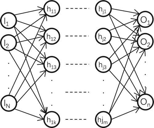
Figure 2. Schematic of DA.

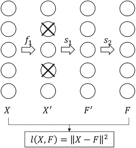
Table 2. Illustration of parameters in DNN.

Variable name	Explanation	Type	Dimensions
$I_i$	the ith neuron of the input layer	symbol	–
$h_j^{\left[i\right]}$	the jth neuron of the ith hidden layer	symbol	–
$O_i$	the ith neuron of the output layer	symbol	–
l	number of DNN layers, excluding the input layer	integer	–
$n^{\left[i\right]}$	number of neurons in the ith layer	integer	–
N	number of input layer neurons, equal to $n^{\left[0\right]}$	integer	–
K	number of output layer neurons, equal to $n^{\left[l\right]}$	integer	–
M	number of samples	integer	–
X	the input sample set	matrix	$N\times M$
$W^{\left[i\right]}$	the weight of the ith layer	matrix	$n^{\left[i\right]}\times n^{[i-1]}$
$b^{\left[i\right]}$	the bias of the ith layer	matrix	$n^{\left[i\right]}\times 1$
$Z^{\left[i\right]}$	the linear output of the ith layer	matrix	$n^{\left[i\right]}\times M$
$a^{\left[i\right]}$	the output of the ith layer	matrix	$n^{\left[i\right]}\times M$
$\hat{y}$	the output of the output layer, equal to $a^{\left[l\right]}$	matrix	$K\times M$
y	the label set corresponding to sample set	matrix	$K\times M$
$g^{\left[i\right]}\left(x\right)$	the activation function of the ith layer	function	–

3.2. Fingerprinting train positioning model

Fading is caused when electromagnetic propagating in space. Theoretically, the farther away from the transmitting terminal, the lower the RSSI received by the receiving terminal. This phenomenon also exists in the urban rail transit environment where using WLAN for communication. Besides, the position of every AP box will not change after the design of signalling system has been completed. Therefore, each AP has different RSSI at different positions, but there is also some complex relationship between RSSI and position. Next, we will model the complex relationship and find it out.

The total number of APs on both sides of the route is N, and the RSSI of all the APs collected by receiving terminal on the train at time t is matrix $X_t=[x_{t1},x_{t2},,x_{tN}{]}^T$, where $x_{ti}$ represents the RSSI of the ith AP at time t. We divide the track into several discrete sections with equal length and represent train position with the section where the train belongs to. In this way, the discrete train sections can be considered as the output of DNN in classification. Besides, in the research on the energy-efficient operation of metro train, knowing which stations the train is located in is sufficient. So the discrete sections can meet the above requirement. Another point, we can conveniently try different section length to improve the positioning accuracy gradually. So in our model, the track is divided into K sections with equal length L. At this time, the train position $p_t$ can be represented by the section $B_i(i=1,2,\dots ,K)$ where the train belongs to. Then the relationship between train position $p_t$ and RSSI at time t can be expressed as $p_t=f\left(X_t\right)$. Here, $p_t$ and $B_i$ both indicate the train position. Their relationship can be expressed as $p_t\in B,B=\{B_1,B_2,\dots ,B_K\}$. The $f\left(x\right)$ is related to channel fading model, train position, AP position and so on, it is difficult to find the exact expression of $f\left(x\right)$. But through deep learning, we can use DNN to gradually approach $f\left(x\right)$. The process of approximation is actually the offline training phase of DNN as shown in Figure 3. The process of feeding the real-time RSSI into the well-trained DNN to output the train position is called the online positioning phase.

Figure 3. Schematic diagram of offline training and online positioning.

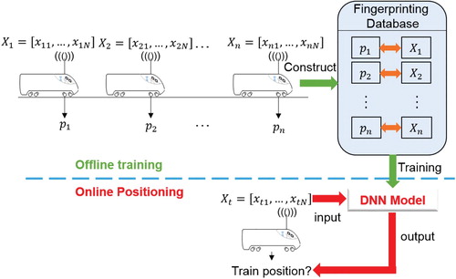
In the offline training phase, the fingerprinting database is constructed by the RSSI matrices and its corresponding positions. These corresponding positions are called labels. The RSSI matrices and the corresponding positions are respectively input matrices and labels of the proposed DNN model. Combined with the introduction to DNN in the previous section, the input matrix of DNN in our model is $X_t=[x_{t1},x_{t2},\dots ,x_{tN}{]}^T$, the number of neurons in input layer is equal to N. The output layer gives the probability of the train in different sections, which can be expressed as Equation 5(5) $\hat{y}=\left[P\right(B_1|X_t),P(B_2|X_t),\dots ,P(B_K|X_t){]}^T,$(5) . (5) $\hat{y}=\left[P\right(B_1|X_t),P(B_2|X_t),\dots ,P(B_K|X_t){]}^T,$(5) where $P\left(B_i|X_t\right)$ is the probability that the train is located in section $B_i$ when the RSSI matrices are $X_t$.

The number of neurons in output layer is equal to K. The section with maximum probability is selected as the predictive value of the final train position by Equation 6(6) $p_t=\mathrm{argmax}(P\left(B_i|X_t\right))i\in [1,K],$(6) . (6) $p_t=\mathrm{argmax}(P\left(B_i|X_t\right))i\in [1,K],$(6) where $\mathrm{argmax}\left(x_i\right)$ returns i that makes the $x_i$ maximum value

Each training set corresponds to one label. In our model, the label is the serial number of the section. When the number of training set is M, the label matrices can be denoted as $label=[p_1,p_2,\dots ,p_M]$. In order to match the label directly with the DNN output, we need to process the label with One Hot Encoding.

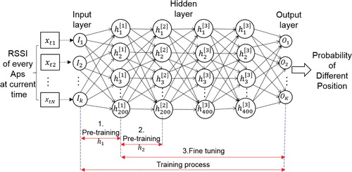
In addition to the input and output layers of the DNN, it is also necessary to specify the parameters of the hidden layers. In our model, the entire neural network have five layers (excluding the input layer) and the number of hidden layers is four. The number of neurons in each hidden layer is $[200,200,400,400]$. The first two hidden layers, $h^{\left[1\right]}$ and $h^{\left[2\right]}$, are set as pre-training layers. The activation function of the hidden layers adopts relu (Glorot, Bordes, & Bengio, 2011) activation function, which is shown in Equation 7(7) $\begin{array}{rl}\mathrm{relu}\left(x\right)& =max(0,x),\end{array}$(7) , and in order to get a multi-category result, the softmax function is used in output layer, which is shown in Equation 8(8) $\begin{array}{rl}\widehat{y_j}& =\frac{{\mathrm{e}}^{z_j^{\left[l-1\right]}}}{\sum _{k=1}^K{\mathrm{e}}^{z_{jk}^{\left[l-1\right]}}},\end{array}$(8) . The Equation 9(9) $\begin{array}{rl}\sum _{k=1}^K{\hat{y}}_{jk}& =1,\end{array}$(9) means that the sum of the probabilities of all categories is 1. The SDA algorithm is used to initialize parameters of hidden layers $h^{\left[1\right]}$ and $h^{\left[2\right]}$. Then the Adam optimization algorithm and the gradient descent algorithm are used to fine tune the entire DNN parameters. The cost function is the cross-entropy cost function, which is shown in Equation 10(10) $\begin{array}{rl}J(\hat{y},y)& =-\frac{1}{m}\sum _{j=1}^m\sum _{k=1}^K(y_{jk}\ln {\hat{y}}_{jk}+(1-y_{jk})(1-\ln {\hat{y}}_{jk})),\end{array}$(10) . When the error of the DNN output meets expectations or no longer changes, the training phase can be considered to be ended. Then we can get a set of trained DNN parameters which can approximately describe the $f\left(X_t\right)$ so that the RSSI can be associated with train position. The DNN structure and training process are shown in Figure 4. (7) $\begin{array}{rl}\mathrm{relu}\left(x\right)& =max(0,x),\end{array}$(7) (8) $\begin{array}{rl}\widehat{y_j}& =\frac{{\mathrm{e}}^{z_j^{\left[l-1\right]}}}{\sum _{k=1}^K{\mathrm{e}}^{z_{jk}^{\left[l-1\right]}}},\end{array}$(8) (9) $\begin{array}{rl}\sum _{k=1}^K{\hat{y}}_{jk}& =1,\end{array}$(9) (10) $\begin{array}{rl}J(\hat{y},y)& =-\frac{1}{m}\sum _{j=1}^m\sum _{k=1}^K(y_{jk}\ln {\hat{y}}_{jk}+(1-y_{jk})(1-\ln {\hat{y}}_{jk})),\end{array}$(10)

Figure 4. DNN training process.

In the online positioning phase, the real-time RSSI collected by the receiving terminal is feed to the trained DNN, then the DNN can output the predictive current train position.

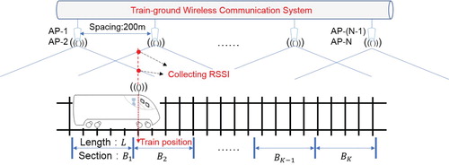
3.3. Simulation verification

The simulation environment for urban rail transit is shown in Figure 5. The track is a straight line with no gradient and is 1000 metres long. For simulating the actual environment, every AP box has 2 APs inside and the spacing of adjacent AP box is 200 metres. In our scene, transmission delay between AP (transmitting terminal) and train (receiving terminal) can be calculated by d/c, where d is the distance between AP and train, c is the speed of light. Therefore, the transmission delay is so short that we can ignore its effect on train position. But on the other hand, the transmission delay is also one of the reasons that may cause multipath (Moghaddam, Amindavar, & Kirlin, 2003). In the NLOS environment, the multipath always exists and makes the RSSI changing. So we cannot ignore the effect of transmission delay on RSSI. In our model, after considering the transmission delay, the RSSI at different positions can be calculated by a NLOS-applicable path loss model by Equation 11(11) $PL\left(d\right)=PL\left(d_0\right)+10n\lg \left(\frac{d}{d_0}\right)+X_{{\sigma }^2},$(11) (Tahat et al., 2017). (11) $PL\left(d\right)=PL\left(d_0\right)+10n\lg \left(\frac{d}{d_0}\right)+X_{{\sigma }^2},$(11) where $X_{{\sigma }^2}$ is a zero mean Gaussian random variable with a variance of ${\sigma }^2$, $d_0$(m) is a short reference distance, d(m) is the distance from AP to train, and n is the path loss exponent.

Figure 5. Schematic of simulation environment.

The path loss exponent n in the tunnel environment is set to 2.073 in the near zone, 1.738 in the far zone (Wang, Ning, Jiang, & Liu, 2013), and the turning point of the near zone and the far zone is set to 100 metres. According to this path loss model, $RSS\left(d\right)$, the RSSI at distance d, can be calculated by Equation 12(12) $\mathrm{RSS}\left(d\right)=\mathrm{RSS}\left(d_0\right)-10n\lg \left(\frac{d}{d_0}\right)+X_{{\sigma }^2},$(12) . (12) $\mathrm{RSS}\left(d\right)=\mathrm{RSS}\left(d_0\right)-10n\lg \left(\frac{d}{d_0}\right)+X_{{\sigma }^2},$(12) The $RSS\left(d_0\right)$ which represents the RSSI at distance $d_0$ from AP can be calculated by the transmitting power of AP $P_{AP}$ and the free space path loss model Equation (13(13) $Ls\left(d\right)=32.45+20\lg f+20\lg d,$(13) ). (13) $Ls\left(d\right)=32.45+20\lg f+20\lg d,$(13) where f(MHz) is the electromagnetic wave frequency, d(Km) is the distance from transmitting terminal and $Ls\left(d\right)$ is the loss power at distance d in free space.

In our simulation, $d_0$ is set to 10 metres, f is 2.4 Ghz, and the transmitting power $P_{AP}$ is equal to 30 mW, which is about 14.77 dBm. Therefore, (14) $\mathrm{RSS}\left(d_0\right)=P_{AP}-Ls\left(d_0\right)=14.77-60.05=-45.28\mathrm{dbm},$(14) Now the only two unknown parameters in Equation 12(12) $\mathrm{RSS}\left(d\right)=\mathrm{RSS}\left(d_0\right)-10n\lg \left(\frac{d}{d_0}\right)+X_{{\sigma }^2},$(12) are d and $X_{{\sigma }^2}$. In our simulation, the ${\sigma }^2$ is set to 5. So the RSSI matrix can be calculated by giving the distance of different APs. In our simulation, we take 1 metre as the sampling interval, one simulation of the train operation can get 1001 RSSI matrices at different positions. The position of the receiving terminal is located at the front of the train and its position is regarded as the position of the train. It should be noted that when the RSSI of some APs is less than $-70$ dBm (based on the AP coverage), the AP is considered out of the coverage of receiving terminal and its RSSI at this time is fixed at $-70$ dBm.

Based on the above simulation, a sufficient fingerprinting database can be established and the DNN network can be trained with the fingerprinting database. The training data can be divided into training set (90% of the database), validation set (5% of the database) and test set (5% of the database). In order to improve training speed and prevent overfitting, the training set is randomly disrupted and divided into some mini bathes. Each mini batch contains 2048 RSSI matrices.

After many attempts, the neurons in pre-training layers are randomly set to zero by the probability of 10%. The number of pre-training times is 200, and the learning rate is 0.001. The learning rate of the fine-tuning phase is also set to 0.001. The hyper parameters ${\beta }_1$, ${\beta }_2$ and ϵ in Adam optimization algorithm are respectively set to 0.9, 0.999, ${10}^{-8}$. After each training, we can get a series of output of DNN. Then the corresponding labels in validation set are used to calculate the model error rate. When the error rate does not decrease for 50 consecutive times, it is considered that the fine-tuning phase is completed. Early stopping can save the training time and avoid overfitting.

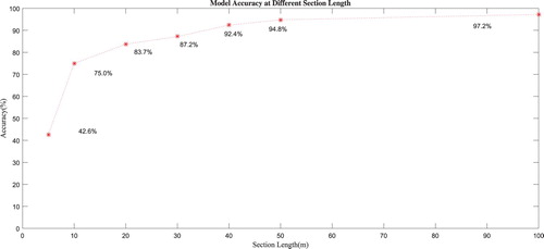
The DNN structure and training algorithm are implemented with tensorflow, and CUDA GPU acceleration technology is used to accelerate the training process. As described above, if we choose a longer section length, when the track length is fixed, we get fewer sections. When section length approaches the track length, there is only one section. In this situation, the output of DNN will be always equal to the label, the train position can be everywhere in the track. So there is a qualitative analysis: when the section length is chosen to be longer, the number of sections is fewer, the accuracy of the DNN model is higher and the position resolution is worse. So we compare model results in different section length. When the section length L is 5, 10, 20, 30, 40, 50 and 100 m respectively, the accuracy of the model is shown in Figure 6. The results can verify the qualitative analysis.

Figure 6. Model accuracy with different section lengths.

Because the train is moving in normal situations, we also analyse the model accuracy at different train velocity. But system delay (the time of once signal scanning) exists in practice. System delay is about 1 sec and its influence on train position can be partially reduced by a position-recursive method (Nguyen, Recalde, & Nashashibi, 2017). In our research, the positioning method is range-free, we cannot get the exact train position, so the recursion is not feasible. Considering the energy-efficient operation research, knowing which two stations the train is located between is enough. The 1 sec system delay can hardly change the stations even if the train is moving at maximum velocity. Therefore, we think that the train position corresponding to the collected RSSI is the true position of the train at the current time. For weakening the influence of section length on model accuracy, we conduct experiment when section length is 20, 30, 40 and 50 m respectively. When the train passes the whole track at 40, 50, 60 and 70 km/h respectively, the accuracy of the model is shown in Table 3. The results show that the model accuracy is slightly lower when velocity is considered. Comparing the results at different situations, we conclude that the section length is the main factor affecting the model accuracy.

Table 3. Model accuracy with different section lengths and velocity.

$L\left(m\right)$
$v\left(km/h\right)$	20	30	40	50
40	79.38%	85.4%	88.5%	92.7%
50	82.8%	83.7%	89.4%	91.4%
60	79.7%	84.4%	89.4%	93.3%
70	76.4%	84.5%	90.3%	92.3%

In the existing research, the evaluation of positioning methods is to compare the positioning error at distance scale. However, in our research, since the positioning method is range-free, the quantitative representation of the train position cannot be obtained, so the evaluation is converted to section scale. The simulation results show that we can easily adjust the section length to improve the model accuracy and make it suitable for the research on energy-efficient operation of metro train.

4. Conclusions and future work

In this paper, we explore how wireless positioning technology is applied to train positioning in urban rail transit, and propose a low-cost fingerprinting train positioning algorithm based on deep learning, which can be used in both ground and underground. The simulation results show that it can satisfy the research on energy-efficient operation of metro train. And the model accuracy is mainly influenced by section length: the longer the section length is, the higher accuracy the model can achieve. Because the proposed positioning method is range-free, the exact train position is not clear. In the future, this method can be integrated with some other positioning methods such as IMU positioning to reduce cumulative error. Besides, with the development of deep learning technologies, some other deep learning architectures can be used such as Recurrent Neural Network to further improve the model accuracy.

Disclosure statement

No potential conflict of interest was reported by the authors.

Additional information

Funding

This work is supported by the Beijing Laboratory of Urban Rail Transit, the Beijing Key Laboratory of Urban Rail Transit Automation and Control, the Research and Demonstration of Key Technologies for Train Traction Energy Consumption Measurement in Urbain Rail Transit, the Fundamental Research Funds for Universities [Grant No. 2018JBZ006], the research funds of National Natural Science Foundation of China [Grant No. 61790570, 61790573], and the State Key Laboratory of Rail Traffic Control and Safety (Beijing Jiaotong University) [Grant No. RCS2018ZT012].

References

- Gao, Y., Zhang, Q., & Chen, L. J. (2018). Formal analysis for reliability and safety of China-Radio in train control system. Journal of Beijing Jiaotong University, 42(2), 61–68.
- Glorot, X., Bordes, A., & Bengio, Y. (2011). Deep sparse rectifier neural networks. Proceedings of Machine Learning Research, 15, 315–323.
- He, Z., Luo, Y., & Zheng, J. (2014). An in-depot realtime train tracking system using rfid and wireless mesh networks. IEEE international conference on intelligent transportation systems (pp. 2404–2409).
- Javed, A., Zhang, H., Huang, Z., & Deng, J. D. (2014). Bws: Beacon-driven wake-up scheme for train localization using wireless sensor networks. IEEE international conference on communications (pp. 276–281).
- Kingma, D. P., & Ba, J. (2014). Adam: A method for stochastic optimization. arXiv preprint arXiv:1412.6980.
- Lee, L. T., & Tsang, K. F. (2008). An active rfid system for railway vehicle identification and positioning. International conference on railway engineering – challenges for railway transportation in information age (pp. 1–4).
- Li, C. R., Xie, J. L., & Yang, L. L. (2015). Angle offset-assisted positioning of railway vehicles in tunnel environments. Vehicular technology conference (pp. 1–5).
- Lin, H., Ye, L., & Wang, Y. (2010). UWB, multi-sensors and wifi-mesh based precision positioning for urban rail traffic. 4633:1–8.
- Miguel, G. D., Goya, J., Uranga, J., Alvarado, U., Adin, I., & Mendizabal, J. (2017). GNSS complementary positioning system performance in railway domain. International conference on ITS telecommunications (pp. 1–7).
- Moghaddam, P. P., Amindavar, H., & Kirlin, R. L. (2003). A new time-delay estimation in multipath. IEEE Transactions on Signal Processing, 51(5), 1129–1142. doi: 10.1109/TSP.2003.810290
- Nguyen, D. V., Recalde, M. E. V., & Nashashibi, F. (2017). Low speed vehicle localization using wifi fingerprinting. International conference on control, automation, robotics and vision (pp. 1–5).
- Tahat, A., Kaddoum, G., Yousefi, S., Valaee, S., & Gagnon, F. (2017). A look at the recent wireless positioning techniques with a focus on algorithms for moving receivers. IEEE Access, 4, 6652–6680. doi: 10.1109/ACCESS.2016.2606486
- Vijayakumar, J. V. N., Zhang, H., Huang, Z., & Javed, A. (2013). A particle filter based train localization scheme using wireless sensor networks. IEEE international conference on dependable, autonomic and secure computing (pp. 269–274).
- Vincent, P., Larochelle, H., Bengio, Y., & Manzagol, P. A. (2008). Extracting and composing robust features with denoising autoencoders. International conference on machine learning (pp. 1096–1103).
- Wang, H., Ning, B., Jiang, H., & Liu, W. (2013). Research on propagation characteristics of 2.4 ghz wlan in tunnels for CBTC train ground communication systems. Journal of the China Railway Society, 35(10), 52–58.
- Weber, R., Mademann, E., Micnler, O., & Zeisberg, S. (2012). Localization techniques for traffic applications based on robust WECOLS positioning in wireless sensor networks. Positioning navigation and communication (pp. 215–219).
- Xiong, L., Zhu, G., & Tan, Z. (2004). Analysis of mobile phone positioning in railway traffic. Journal of the China Railway Society, 26(1), 73–76.