High-resolution imaging algorithm based on temporal focal characteristic of time-reversed signal

Abstract

Although the high-resolution materials can improve the resolution of the conventional time-reversal imaging (TRI) algorithms, they also limit the applications of TRI. In this paper, a new TRI algorithm with high-resolution is presented. Since the proposed algorithm utilizes multiple time reversal operation steps to improve resolution, it can realize high-resolution without invoking any high-resolution materials. The results show the resolution of the proposed algorithm is superior to that of the conventional TRI.

KEYWORDS:

• High-resolution
• imaging algorithm
• time-reversal

1. Introduction

The time-reversal technique (Fink, 1992; Wu, Thomas, & Fink, 1992) makes use of reciprocity of wave propagation in a time-invariant medium. In recent years, This method has attracted significant attention in many applications, such as communication (Wu et al., 2019; Yang, Wang, & Ding, 2018), imaging (Gao, Zhang, Li, Huo, & Song, 2017; Li & Hu, 2015), and nondestructive detection (Huo, Wang, Chen, & Song, 2017; Liang, Feng, & Li, 2018; Zhang, Zhu, Song, Peng, & Song, 2018).

The concept of time reversal (TR) is based on the spatial reciprocity (Fink, 1992). The self-adapting spatial and temporal focusing characteristic occurs at the excitation location when the signals recorded by transducers are time reversed in the time domain (or phase conjugated in frequency domain) and emitted back at the transducer locations (Fink, 1997). Time-reversal imaging technology computationally re-radiated the signals into the domain of interest in a computer instead of implemented in a real medium. In computation process, the time-reversed signals are multiplied with the transfer function (usually, use Green function as transfer function) in frequency domain (Liu, Kang, Li, & Chen, 2005). Of course, the same process can also be done by convoluting the time-reversed signal with channel impulse response which is the inverse Fourier transform of transfer function (Ing, Quieffin, Catheline, & Fink, 2005; Liu et al., 2005), since the multiplication in frequency domain equals to the convolution in time domain. Some investigators used the time-reversed signal amplitude at the prospective time to reconstruct the defect image map. Based on the measured signals, Amitt et al. performed a computational TR run, and obtained a solution at the reversed time t = T (Amitt, Dan, & Turkel, 2014). Several localization methods based on the similar principle were developed for SHM systems with the distributed sensor/actuator networks (Cai, Shi, & Yuan, 2011; Wang, Rose, & Chang, 2004). Another detection method of TR is based on the maximum time-reversed signal value. R.K. Ing et al. used a maximum of TR energy to identify the position where the finger knocked (Ing et al., 2005). In concrete model, the maximum value of the TR energy is used to locate the source's position (Kocur, Vogel, & Saenger, 2011; Saenger, Kocur, Jud, & Torrilhon, 2011). Zhao et al. utilized the maximum of the displacement field in the revered time domain to build the defect image (Zhao, Zhang, Zhang, & Wang, 2018).

The increase of the effective array size can improve the resolution of the time-reversal imaging (TRI) algorithm, since the channel information can be collected more completely with larger aperture width (Fouque, Garnier, Papanicolaou, & Sølna, 2007; Lerosey et al., 2004; Liao, Hsieh, & Chen, 2009; Matthieu, Stefan, & Philippe, 2015). In order to produce a larger aperture width, one current high-resolution method is to increase receiver elements of the array (Liao et al., 2009). The other is to use the so-called high-resolution materials when detecting the targets (Grbic & Elefteriades, 2004; Lemoult, Lerosey, de Rosny, & Fink, 2010; Matthieu et al., 2015). Compared to actually increase the physical aperture size of the array, the high-resolution materials are considered as more economical solutions and therefore become a popular topic in recent years. One kind of the high-resolution materials consists of subwavelength resonant structures, such as metallic cylinders arrays (Gao, Wang, & Wang, 2015; Gong et al., 2017; Lemoult, Fink, & Lerosey, 2012; Wang, Wang, Gong, & Ding, 2015). Those high-resolution materials can convert evanescent waves into propagating waves, which can then be detected in the far field, in order to increase the subwavelength information about an object. By means of the subwavelength information, TR can achieve subwavelength focusing effects. The other kind of the high-resolution materials is composed of a multilayered medium or a continuous random media (Liao et al., 2009). The multilayered medium or the continuous random media can enhance the multipath effect. With the aid of that materials, the TR techniques based on a multilayered medium or a continuous random media can also reach high-resolution.

Although the high-resolution materials can improve resolution, they also bring several shortcomings. Firstly, for converting evanescent waves into propagating waves effectively, the high-resolution materials have to be very close to the targets (usually, the distance between the high-resolution materials and the target is much less than $\lambda$) (Grbic & Elefteriades, 2004; Lemoult et al., 2010; Lemoult et al., 2012). In Lemoult et al. (2010), the source is 2 mm (about $6.7\times {10}^{-4}\lambda$) away from the resonant metalen. In Grbic and Elefteriades (2004), a vertical monopole is attached directly to the left-handed slab, which means the distant between the target and the slab is zero. The investigators placed an object in the focal plane of the resonant metalens, that is, 25 nm (about 0.036$\lambda$) above it (Lemoult et al., 2012). On the other hand, since the high-resolution materials result in the loss and the dispersion (Gong et al., 2017; Lemoult et al., 2012), they will also deteriorate the signal energy transmission coefficient.

Undoubtedly, TR imaging techniques become more practical and exploitable if high-resolution is obtained without invoking any high-resolution materials. For that purpose, a new TR imaging algorithm is developed. The proposed algorithm uses multiple time reversal operation steps to provide higher resolution that cannot be obtained by using the conventional imaging method. The results show the proposed algorithm can even distinguish the two targets separated by a distance of 0.18$\lambda$ without invoking any high-resolution materials. Furthermore, since the proposed method only optimizes the calculation process, it can be associated with the high-resolution materials, in order to obtain higher resolution (Zhang & Song, 2017a, 2017b; Zhang, Ho, Huo, & Zhu, 2019).

2. Theory

In this paper, the conventional TRI based on the focal time is employed for comparison. Therefore, the conventional TRI and the proposed method are described respectively in this section.

2.1. Time-reversal theory

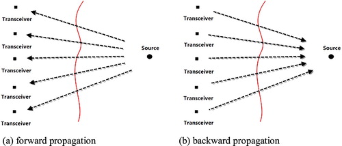
The basic principle of TR is shown in Figure 1. Assume a localized source, with the radiated time-domain fields measured by an array of transceivers. The received data are time reversed (or phase conjugated in the frequency domain) and radiated from the respective transceiver locations. If the channels in the area are invariant in time, the re-radiated signals focus at the source point, and the characteristics of the temporal source are recovered, according to the spatial reciprocity principle.

Figure 1. Schematic of time-reversal process. A time-domain source emits a signal received by a transceiver array. The signals are reversed in time and radiated into the domain. (a) Forward propagation, (b) backward propagation.

2.2. The conventional TRI and the novel imaging method

For convenience of description, consider a 2-D imaging model. Assume an array of $N$transceivers is used, and the $n^{th}$ transceiver’s receiver and transmitter are located at ${\mathbf{\text{r}}}_{\mathbf{\text{n}}}$ and ${\mathbf{\text{r}}}_{\mathbf{\text{n}}}^{\mathrm{\prime }}$, respectively. Consider the scatterer with the scattering potential $\rho \left({\mathbf{\text{r}}}_{\mathbf{\text{s}}}\right)$ located at ${\mathbf{\text{r}}}_{\mathbf{\text{s}}}$, plain symbols denote scalar quantities, whereas vectors and matrices are denoted by bold symbols, and this will be used throughout the paper.

A probing pulse $x\left(t\right)$ is emitted from the transmitter positioned at ${\mathbf{\text{r}}}_{\mathbf{\text{n}}}^{\mathrm{\prime }}$. The frequency-domain representation of the incident signal at ${\mathbf{\text{r}}}_{\mathbf{\text{s}}}$ is, (1) $E\left(\omega ,{\mathbf{\text{r}}}_{\mathbf{\text{s}}}\right)=G_{\mathbf{\text{u}}}\left({\mathbf{\text{r}}}_{\mathbf{\text{s}}},{{\mathbf{\text{r}}}^{\mathrm{\prime }}}_{\mathbf{\text{n}}},\omega \right)X\left(\omega \right)$(1) where $X\left(\omega \right)$ is the Fourier transform of $x\left(t\right)$ and $G_{\mathbf{\text{u}}}({\mathbf{\text{r}}}_{\mathbf{\text{s}}},{\mathbf{\text{r}}}_{\mathbf{\text{n}}}^{\mathrm{\prime }},\omega )$ is the Green function representing the ‘propagator' from location ${\mathbf{\text{r}}}_{\mathbf{\text{n}}}^{\mathrm{\prime }}$ to ${\mathbf{\text{r}}}_{\mathbf{\text{s}}}$, obtained by measurement.

The Fourier transform of the echo signal recorded by the corresponding receiver could be modelled as, (2) $Y(\omega ,{\mathbf{\text{r}}}_{\mathbf{\text{n}}},{\mathbf{\text{r}}}_{\mathbf{\text{n}}}^{\mathrm{\prime }})=G_{\mathbf{\text{u}}}({\mathbf{\text{r}}}_{\mathbf{\text{n}}},{\mathbf{\text{r}}}_{\mathbf{\text{s}}},\omega )G_{\mathbf{\text{u}}}({\mathbf{\text{r}}}_{\mathbf{\text{s}}},{\mathbf{\text{r}}}_{\mathbf{\text{n}}}^{\mathrm{\prime }},\omega )\rho \left({\mathbf{\text{r}}}_{\mathbf{\text{s}}}\right)X\left(\omega \right)$(2)

Since the time reversal of a signal is equivalent to taking the complex conjugate in the frequency domain, the time-reversal version of (2) can be represented as, (3) $Y_{\mathbf{\text{TR}}}(\omega ,{\mathbf{\text{r}}}_{\mathbf{\text{n}}},{\mathbf{\text{r}}}_{\mathbf{\text{n}}}^{\mathrm{\prime }})={G_{\mathbf{\text{u}}}}^{\ast }({\mathbf{\text{r}}}_{\mathbf{\text{n}}},{\mathbf{\text{r}}}_{\mathbf{\text{s}}},\omega ){G_{\mathbf{\text{u}}}}^{\ast }({\mathbf{\text{r}}}_{\mathbf{\text{s}}},{\mathbf{\text{r}}}_{\mathbf{\text{n}}}^{\mathrm{\prime }},\omega )\rho \left({\mathbf{\text{r}}}_{\mathbf{\text{s}}}\right)X^{\ast }\left(\omega \right)$(3) where ‘*' represents the complex conjugate.

2.2.1. The conventional TRI

In conventional TRI algorithm, the time-reversed signals are numerically rebroadcasted from each receiver's location (Shi & Nehorai, 2007; Wang et al., 2015). For a generic observation point ${\mathbf{\text{r}}}_{\mathbf{\text{k}}}$, the time-reversed signal of the array can be presented as following, (4) $\begin{array}{rl}{y}_c({\mathbf{\text{r}}}_k,t)& =\frac{1}{2\pi }{\int }_{}^{}\left[\sum _{n=1}^N{G_{\mathbf{\text{u}}}}^{\ast }({\mathbf{\text{r}}}_{\mathbf{\text{n}}},{\mathbf{\text{r}}}_{\mathbf{\text{s}}},\omega ){G_{\mathbf{\text{u}}}}^{\ast }({\mathbf{\text{r}}}_{\mathbf{\text{s}}},{{\mathbf{\text{r}}}^{\mathrm{\prime }}}_{\mathbf{\text{n}}},\omega )\right.\\ & \left.G_{\mathbf{\text{v}}}({\mathbf{\text{r}}}_{\mathbf{\text{n}}},{\mathbf{\text{r}}}_{\mathbf{\text{k}}},\omega )G_{\mathbf{\text{v}}}({\mathbf{\text{r}}}_{\mathbf{\text{k}}},{{\mathbf{\text{r}}}^{\mathrm{\prime }}}_{\mathbf{\text{n}}},\omega )\right]\times \rho \left({\mathbf{\text{r}}}_{\mathbf{\text{s}}}\right)X^{\ast }\left(\omega \right){\mathrm{e}}^{i\omega t}d\omega \end{array}$(4) where $G_{\mathbf{\text{v}}}({\mathbf{\text{r}}}_{\mathbf{\text{n}}},{\mathbf{\text{r}}}_{\mathbf{\text{k}}},\omega )$ is the computational Green function representing the ‘propagator' from location ${\mathbf{\text{r}}}_{\mathbf{\text{n}}}$ to a generic observation point ${\mathbf{\text{r}}}_{\mathbf{\text{k}}}$. The subscript ‘v' represents that this corresponds to the back-propagation fields, computed in software.

In the conventional TRI, the signal value at t = 0 is used as the pixel value. As a result, the imaging functional of the conventional TRI algorithm for point ${\mathbf{\text{r}}}_{\mathbf{\text{k}}}$ in the image domain is, (5) $\begin{array}{rl}{I}_c\left({\mathbf{\text{r}}}_k\right)& =\frac{1}{2\pi }{\int }_{}^{}\left[\sum _{n=1}^N{G_{\mathbf{\text{u}}}}^{\ast }({\mathbf{\text{r}}}_{\mathbf{\text{n}}},{\mathbf{\text{r}}}_{\mathbf{\text{s}}},\omega ){G_{\mathbf{\text{u}}}}^{\ast }({\mathbf{\text{r}}}_{\mathbf{\text{s}}},{{\mathbf{\text{r}}}^{\mathrm{\prime }}}_{\mathbf{\text{n}}},\omega )\right.\\ & \left.G_{\mathbf{\text{v}}}({\mathbf{\text{r}}}_{\mathbf{\text{n}}},{\mathbf{\text{r}}}_{\mathbf{\text{k}}},\omega )G_{\mathbf{\text{v}}}({\mathbf{\text{r}}}_{\mathbf{\text{k}}},{{\mathbf{\text{r}}}^{\mathrm{\prime }}}_{\mathbf{\text{n}}},\omega )\right]\times \rho \left({\mathbf{\text{r}}}_{\mathbf{\text{s}}}\right)X^{\ast }\left(\omega \right)d\omega \end{array}$(5) when the computational Green function matches the measured data, namely $G_{\mathbf{\text{u}}}({\mathbf{\text{r}}}_{\mathbf{\text{n}}},{\mathbf{\text{r}}}_{\mathbf{\text{k}}},\omega )=G_{\mathbf{\text{v}}}({\mathbf{\text{r}}}_{\mathbf{\text{n}}},{\mathbf{\text{r}}}_{\mathbf{\text{k}}},\omega )$, the pixel value at target's location can be expressed as, (6) $\begin{array}{rl}{I}_c\left({\mathbf{\text{r}}}_s\right)& =\frac{1}{2\pi }{\int }_{}^{}\rho \left({\mathbf{\text{r}}}_{\mathbf{\text{s}}}\right)X^{\ast }\left(\omega \right)\sum _{n=1}^N{|G_{\mathbf{\text{u}}}({\mathbf{\text{r}}}_{\mathbf{\text{n}}},{\mathbf{\text{r}}}_s,\omega )|}^2\\ & \times {|G_{\mathbf{\text{u}}}({\mathbf{\text{r}}}_s,{{\mathbf{\text{r}}}^{\mathrm{\prime }}}_{\mathbf{\text{n}}},\omega )|}^{2}d\omega \end{array}$(6)

2.2.2. The novel imaging method

In the proposed method, the transceivers are firstly divided into several sub-arrays (looks), before the signals are time reversed and resubmitted. Each sub-array includes 2 transceivers. Therefore, the number of the sub-arrays is C(N,2), where C(N,2) is the number of 2-combinations from the $N$ transceivers (Gao et al., 2017).

Secondly, assume the $a^{th}$ sub-array is composed of transceiver $m$ and transceiver $j$. We compose a new signal by superposing the echo signals of transceiver $m$ and transceiver $j$. The Fourier transform of the new signal can be represented as (7) $Y_a\left(\omega \right)=Y(\omega ,{\mathbf{\text{r}}}_m,{\mathbf{\text{r}}}_m^{\mathrm{\prime }})+Y(\omega ,{\mathbf{\text{r}}}_j,{\mathbf{\text{r}}}_j^{\mathrm{\prime }})$(7)

Thirdly, the new signal is time reversed and resubmitted at transceiver $m$ and transceiver $j$.

Accounting for back-propagation from the transmitter at ${\mathbf{\text{r}}}_m^{\mathrm{\prime }}$ and the receiver at ${\mathbf{\text{r}}}_m$ to any point ${\mathbf{\text{r}}}_{\mathbf{\text{k}}}$ in the image domain, the Fourier transform of the time reversal signal $f_m^a(t,{\mathbf{\text{r}}}_{\mathbf{\text{k}}},{\mathbf{\text{r}}}_m,{\mathbf{\text{r}}}_m^{\mathrm{\prime }})$ for a generic observation point ${\mathbf{\text{r}}}_{\mathbf{\text{k}}}$ can be illustrated as, (8) $\begin{array}{rl}{F}_m^a(\omega ,{\mathbf{\text{r}}}_{\mathbf{\text{k}}},{\mathbf{\text{r}}}_m,{\mathbf{\text{r}}}_m^{\mathrm{\prime }})& =G_{\mathbf{\text{v}}}({\mathbf{\text{r}}}_m,{\mathbf{\text{r}}}_{\mathbf{\text{k}}},\omega )G_{\mathbf{\text{v}}}({\mathbf{\text{r}}}_{\mathbf{\text{k}}},{\mathbf{\text{r}}}_m^{\mathrm{\prime }},\omega )\\ & \times \rho \left({\mathbf{\text{r}}}_{\mathbf{\text{s}}}\right)X^{\ast }\left(\omega \right)Y_a^{\ast }\left(\omega \right)\end{array}$(8)

Accordingly, for transceiver $j$, the Fourier transform of the time-reversed signal $f_j^a(t,{\mathbf{\text{r}}}_{\mathbf{\text{k}}},{\mathbf{\text{r}}}_j,{\mathbf{\text{r}}}_j^{\mathrm{\prime }})$ at the generic observation point ${\mathbf{\text{r}}}_{\mathbf{\text{k}}}$ can be illustrated as, (9) $F_j^a(\omega ,{\mathbf{\text{r}}}_{\mathbf{\text{k}}},{\mathbf{\text{r}}}_j,{\mathbf{\text{r}}}_j^{\mathrm{\prime }})=G_{\mathbf{\text{v}}}({\mathbf{\text{r}}}_j,{\mathbf{\text{r}}}_{\mathbf{\text{k}}},\omega )G_{\mathbf{\text{v}}}({\mathbf{\text{r}}}_{\mathbf{\text{k}}},{\mathbf{\text{r}}}_j^{\mathrm{\prime }},\omega )\rho \left({\mathbf{\text{r}}}_{\mathbf{\text{s}}}\right)X^{\ast }\left(\omega \right)Y_a^{\ast }\left(\omega \right)$(9)

Time reverse $f_j^a(t,{\mathbf{\text{r}}}_{\mathbf{\text{k}}},{\mathbf{\text{r}}}_j,{\mathbf{\text{r}}}_j^{\mathrm{\prime }})$ and calculate the cross-correlation between $f_m^a(t,{\mathbf{\text{r}}}_{\mathbf{\text{k}}},{\mathbf{\text{r}}}_m,{\mathbf{\text{r}}}_m^{\mathrm{\prime }})$ and the time reversal version of $f_j^a(t,{\mathbf{\text{r}}}_{\mathbf{\text{k}}},{\mathbf{\text{r}}}_j,{\mathbf{\text{r}}}_j^{\mathrm{\prime }})$, we can obtain, (10) $\begin{array}{rl}{q}_a({\mathbf{\text{r}}}_{\mathbf{\text{k}}},t)& =f_m^a(t,{\mathbf{\text{r}}}_{\mathbf{\text{k}}},{\mathbf{\text{r}}}_m,{\mathbf{\text{r}}}_m^{\mathrm{\prime }})\otimes f_j^a(t,{\mathbf{\text{r}}}_{\mathbf{\text{k}}},{\mathbf{\text{r}}}_j,{\mathbf{\text{r}}}_j^{\mathrm{\prime }})\\ & =\frac{1}{2\pi }{\int }_{}^{}{F}_m^a(\omega ,{\mathbf{\text{r}}}_{\mathbf{\text{k}}},{\mathbf{\text{r}}}_m,{{\mathbf{\text{r}}}^{\mathrm{\prime }}}_m)F_j^a(\omega ,{\mathbf{\text{r}}}_{\mathbf{\text{k}}},{\mathbf{\text{r}}}_j,{{\mathbf{\text{r}}}^{\mathrm{\prime }}}_j){\mathrm{e}}^{i\omega t}d\omega \end{array}$(10) where ‘$\otimes$’ represents the convolution operation.

By summing over all sub-arrays, we can obtain (11) $q({\mathbf{\text{r}}}_{\mathbf{\text{k}}},t)=\sum _{a=1}^{C\left(N,2\right)}{q}_a({\mathbf{\text{r}}}_{\mathbf{\text{k}}},t)$(11)

Take $q({\mathbf{\text{r}}}_{\mathbf{\text{k}}},0)$ as the pixel value of the generic observation point ${\mathbf{\text{r}}}_{\mathbf{\text{k}}}$, then the imaging functional of the proposed method is written as following, (12) $I_p\left({\mathbf{\text{r}}}_{\mathbf{\text{k}}}\right)=q({\mathbf{\text{r}}}_{\mathbf{\text{k}}},0)$(12)

When the computational Green function matches the measured data, namely $G_{\mathbf{\text{u}}}({\mathbf{\text{r}}}_{\mathbf{\text{n}}},{\mathbf{\text{r}}}_{\mathbf{\text{k}}},\omega )=G_{\mathbf{\text{v}}}({\mathbf{\text{r}}}_{\mathbf{\text{n}}},{\mathbf{\text{r}}}_{\mathbf{\text{k}}},\omega )$, the image of target can be represented as, (13) $\begin{array}{rl}{I}_p\left({\mathbf{\text{r}}}_s\right)& =\frac{1}{2\pi }{\int }_{}^{}\rho {\left({\mathbf{\text{r}}}_{\mathbf{\text{s}}}\right)}^2{X}^{\ast }{\left(\omega \right)}^2\sum _{m=1}^N\sum _{j=1,j\ne m}^N{|G_{\mathbf{\text{u}}}({\mathbf{\text{r}}}_m,{\mathbf{\text{r}}}_s,\omega )|}^2\\ & \times {|G_{\mathbf{\text{u}}}({\mathbf{\text{r}}}_s,{{\mathbf{\text{r}}}^{\mathrm{\prime }}}_m,\omega )|}^2|G_{\mathbf{\text{u}}}({\mathbf{\text{r}}}_j,{\mathbf{\text{r}}}_{\mathbf{\text{s}}},\omega ){|}^2|G_{\mathbf{\text{u}}}({\mathbf{\text{r}}}_{\mathbf{\text{s}}},{{\mathbf{\text{r}}}^{\mathrm{\prime }}}_j,\omega ){|}^{\text{2}}d\omega \end{array}$(13)

2.3. Analysis about resolution

For explain the reason why the resolution is improved, consider a generic observation point ${\mathbf{\text{r}}}_{\mathbf{\text{z}}}$ which is very close to the target, namely ${\mathbf{\text{r}}}_{\mathbf{\text{z}}}\approx {\mathbf{\text{r}}}_{\mathbf{\text{s}}}$. Then, we can get, (14) $\begin{array}{rl}& G_{\mathbf{\text{v}}}({\mathbf{\text{r}}}_{\mathbf{\text{n}}},{\mathbf{\text{r}}}_{\mathbf{\text{z}}},\omega )G_{\mathbf{\text{v}}}({\mathbf{\text{r}}}_{\mathbf{\text{z}}},{\mathbf{\text{r}}}_{\mathbf{\text{n}}}^{\mathrm{\prime }},\omega )\\ & =G_{\mathbf{\text{v}}}({\mathbf{\text{r}}}_{\mathbf{\text{n}}},{\mathbf{\text{r}}}_{\mathbf{\text{s}}},\omega )G_{\mathbf{\text{v}}}({\mathbf{\text{r}}}_{\mathbf{\text{s}}},{\mathbf{\text{r}}}_{\mathbf{\text{n}}}^{\mathrm{\prime }},\omega )b_{\mathbf{\text{n}},\mathbf{\text{s}},\mathbf{\text{z}}}{e}^{i{\theta }_{\mathbf{\text{n}},\mathbf{\text{s}},\mathbf{\text{z}}}}\end{array}$(14) where ${\theta }_{\mathbf{\text{n}},\mathbf{\text{s}},\mathbf{\text{z}}}$ is the phase difference between $G_{\mathbf{\text{v}}}({\mathbf{\text{r}}}_{\mathbf{\text{n}}},{\mathbf{\text{r}}}_{\mathbf{\text{z}}},\omega )G_{\mathbf{\text{v}}}({\mathbf{\text{r}}}_{\mathbf{\text{z}}},{\mathbf{\text{r}}}_{\mathbf{\text{n}}}^{\mathrm{\prime }},\omega )$ and $G_{\mathbf{\text{v}}}({\mathbf{\text{r}}}_{\mathbf{\text{n}}},{\mathbf{\text{r}}}_{\mathbf{\text{s}}},\omega )G_{\mathbf{\text{v}}}({\mathbf{\text{r}}}_{\mathbf{\text{s}}},{\mathbf{\text{r}}}_{\mathbf{\text{n}}}^{\mathrm{\prime }},\omega )$, $b_{\mathbf{\text{n}}}=|G_{\mathbf{\text{v}}}({\mathbf{\text{r}}}_{\mathbf{\text{n}}},{\mathbf{\text{r}}}_{\mathbf{\text{z}}},\omega )G_{\mathbf{\text{v}}}({\mathbf{\text{r}}}_{\mathbf{\text{z}}},{{\mathbf{\text{r}}}^{\mathrm{\prime }}}_{\mathbf{\text{n}}},\omega )|/|G_{\mathbf{\text{v}}}({\mathbf{\text{r}}}_{\mathbf{\text{n}}},{\mathbf{\text{r}}}_{\mathbf{\text{s}}},\omega )G_{\mathbf{\text{v}}}({\mathbf{\text{r}}}_{\mathbf{\text{s}}},{{\mathbf{\text{r}}}^{\mathrm{\prime }}}_{\mathbf{\text{n}}},\omega )|$.

Since ${\mathbf{\text{r}}}_{\mathbf{\text{z}}}\approx {\mathbf{\text{r}}}_{\mathbf{\text{s}}}$, ${\theta }_{\mathbf{\text{n}},\mathbf{\text{s}},\mathbf{\text{z}}}$ approaches to zero, $b_{\mathbf{\text{n}},\mathbf{\text{s}},\mathbf{\text{z}}}$ approaches to one.

By using the conventional TRI, according to (5), the pixel value at ${\mathbf{\text{r}}}_{\mathbf{\text{z}}}$ can be represented as, (15) $\begin{array}{rl}{I}_c\left({\mathbf{\text{r}}}_{\mathbf{\text{z}}}\right)& =\frac{1}{2\pi }{\int }_{}^{}\rho \left({\mathbf{\text{r}}}_{\mathbf{\text{s}}}\right)X^{\ast }\left(\omega \right)\times \sum _{n=1}^N{b}_{\mathbf{\text{n}},\mathbf{\text{s}},\mathbf{\text{z}}}\\ & \times {|G_{\mathbf{\text{u}}}({\mathbf{\text{r}}}_{\mathbf{\text{n}}},{\mathbf{\text{r}}}_s,\omega )|}^2{|G_{\mathbf{\text{u}}}({\mathbf{\text{r}}}_s,{{\mathbf{\text{r}}}^{\mathrm{\prime }}}_{\mathbf{\text{n}}},\omega )|}^2{e}^{i{\theta }_{\mathbf{\text{n}},\mathbf{\text{s}},\mathbf{\text{z}}}}d\omega \end{array}$(15)

From (15), it can be seen that if ${\mathbf{\text{r}}}_{\mathbf{\text{z}}}={\mathbf{\text{r}}}_{\mathbf{\text{s}}}$, ${\theta }_{\mathbf{\text{n}},\mathbf{\text{s}},\mathbf{\text{z}}}$=0, $I_c\left({\mathbf{\text{r}}}_{\mathbf{\text{z}}}\right)$ is $I_c\left({\mathbf{\text{r}}}_{\mathbf{\text{s}}}\right)$ which is the maximum pixel value. When the generic observation point ${\mathbf{\text{r}}}_{\mathbf{\text{z}}}$gets away from the targets, the ${\theta }_{\mathbf{\text{n}},\mathbf{\text{s}},\mathbf{\text{z}}}$ gets larger, and $I_c\left({\mathbf{\text{r}}}_{\mathbf{\text{z}}}\right)/I_c\left({\mathbf{\text{r}}}_{\mathbf{\text{s}}}\right)$ gets smaller. Therefore, for a generic observation point ${\mathbf{\text{r}}}_{\mathbf{\text{z}}}$ which is very close to the target (${\mathbf{\text{r}}}_{\mathbf{\text{z}}}\approx {\mathbf{\text{r}}}_{\mathbf{\text{s}}}$), ${\theta }_{\mathbf{\text{n}},\mathbf{\text{s}},\mathbf{\text{z}}}\approx 0$, $I_c\left({\mathbf{\text{r}}}_{\mathbf{\text{z}}}\right)/I_c\left({\mathbf{\text{r}}}_{\mathbf{\text{s}}}\right)$ is closer to one. There is a very small difference between $I_c\left({\mathbf{\text{r}}}_{\mathbf{\text{s}}}\right)$ and $I_c\left({\mathbf{\text{r}}}_{\mathbf{\text{z}}}\right)$. It is very difficult to identify the target.

By using proposed method, the pixel value at ${\mathbf{\text{r}}}_{\mathbf{\text{z}}}$ can be written as (16) $\begin{array}{rl}{I}_p\left({\mathbf{\text{r}}}_{\mathbf{\text{z}}}\right)& =\frac{1}{2\pi }{\int }_{}^{}\rho {\left({\mathbf{\text{r}}}_{\mathbf{\text{s}}}\right)}^2{X}^{\ast }{\left(\omega \right)}^2\sum _{m=1}^N\sum _{j=1,j\ne m}^N{|G_{\mathbf{\text{u}}}({\mathbf{\text{r}}}_m,{\mathbf{\text{r}}}_s,\omega )|}^2\\ & \times {|G_{\mathbf{\text{u}}}({\mathbf{\text{r}}}_s,{{\mathbf{\text{r}}}^{\mathrm{\prime }}}_m,\omega )|}^2|G_{\mathbf{\text{u}}}({\mathbf{\text{r}}}_{\mathbf{\text{j}}},{\mathbf{\text{r}}}_{\mathbf{\text{s}}},\omega ){|}^2\\ & \times |G_{\mathbf{\text{u}}}({\mathbf{\text{r}}}_{\mathbf{\text{s}}},{{\mathbf{\text{r}}}^{\mathrm{\prime }}}_{\mathbf{\text{j}}},\omega ){|}^{\text{2}}{b}_{\mathbf{\text{j}},\mathbf{\text{s}},\mathbf{\text{z}}}{b}_{\mathbf{\text{m}},\mathbf{\text{s}},\mathbf{\text{z}}}{e}^{i\left({\theta }_{\mathbf{\text{m}},\mathbf{\text{s}},\mathbf{\text{z}}}+{\theta }_{\mathbf{\text{j}},\mathbf{\text{s}},\mathbf{\text{z}}}\right)}d\omega \end{array}$(16)

The phase difference between $I_p\left({\mathbf{\text{r}}}_{\mathbf{\text{z}}}\right)$ and $I_p\left({\mathbf{\text{r}}}_s\right)$ is the total of ${\theta }_{\mathbf{\text{m}},\mathbf{\text{s}},\mathbf{\text{z}}}$ and ${\theta }_{\mathbf{\text{j}},\mathbf{\text{s}},\mathbf{\text{z}}}$. Therefore, the phase difference between $I_p\left({\mathbf{\text{r}}}_{\mathbf{\text{z}}}\right)$ and $I_p\left({\mathbf{\text{r}}}_s\right)$ is larger than that between $I_c\left({\mathbf{\text{r}}}_{\mathbf{\text{s}}}\right)$ and $I_c\left({\mathbf{\text{r}}}_{\mathbf{\text{z}}}\right)$. For${\mathbf{\text{r}}}_{\mathbf{\text{z}}}\approx {\mathbf{\text{r}}}_{\mathbf{\text{s}}}$, $I_p\left({\mathbf{\text{r}}}_{\mathbf{\text{z}}}\right)/I_p\left({\mathbf{\text{r}}}_{\mathbf{\text{s}}}\right)<I_c\left({\mathbf{\text{r}}}_{\mathbf{\text{z}}}\right)/I_c\left({\mathbf{\text{r}}}_{\mathbf{\text{s}}}\right)$. Obviously, the attenuation of the pixel value based on the proposed method is faster than that based on the conventional TRI, for the points close to the target. As a result, the target can be revealed more easily by using the proposed method, the resolution of the proposed method is higher.

3. Numerical experiment and discussion

A numerical experiment was taken in the following section.

The Gaussian pulse with the central frequency 6.85 GHz and a frequency band ranging 3–10.7 GHz was used as the UWB excitation. The size of the detection array composed of eight transceivers is 28 cm. The specific positions of the transceivers are listed as Table 1. Two targets’ sizes are 2 mm$\times$2 mm. The positions of the two targets are set in three cases, as shown in Table 2. The vertical distance between the targets and the array is 28 cm. In order to facilitate comparison, all echo signals will be processed by using the proposed algorithm and the conventional TRI algorithm.

Table 1. The specific locations of transceivers in the experiment, units: m.

Transceivers	Locations
Transceiver 1	X = −0.14,	Y = 0
Transceiver 2	X = −0.1,	Y = 0
Transceiver 3	X = −0.06,	Y = 0
Transceiver 4	X = −0.02,	Y = 0
Transceiver 5	X = 0.02,	Y = 0
Transceiver 6	X = 0.06,	Y = 0
Transceiver 7	X = 0.1,	Y = 0
Transceiver 8	X = 0.14,	Y = 0

Table 2. The specific locations of the two targets in numerical experiment, units: m.

Cases	Target 1's location	Target 2's location
Case 1	X = −0.016, Y = 0.28	X = 0.028, Y = 0.28
Case 2	X = −0.008, Y = 0.28	X = 0.014, Y = 0.28
Case 3	X = −0.008, Y = 0.28	X = 0.01, Y = 0.28

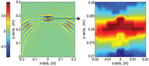
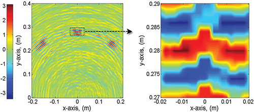
In case 1, the distance between the two targets is about $\lambda$. As shown in Figures 2 and 3, although the targets can be distinguished from the imaging maps obtained by the both algorithms, the proposed algorithm can reach higher resolution.

Figure 2. The proposed algorithm's imaging results in case 1 at noise free.

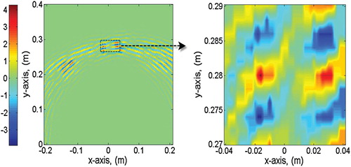
Figure 3. The conventional TRI's imaging results in case 1 at noise free.

In case 2, the distance between two targets decreases to 0.5$\lambda$ in the simulation domain, the distance at which the time reversal signals cannot retro-focus in the free space (Liao et al., 2009). The results obtained by both algorithms are shown in Figures 4 and 5. It can be found that the conventional TRI algorithm cannot identify the two targets. In contrast, the proposed algorithm can still focus at two pixels and show a cleaner image.

Figure 4. The proposed algorithm's imaging results in case 2 at noise free.

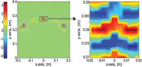
Figure 5. The conventional TRI's imaging results in case 2 at noise free.

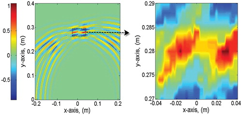
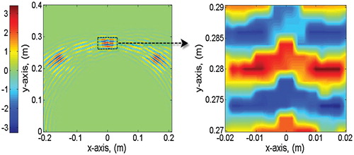
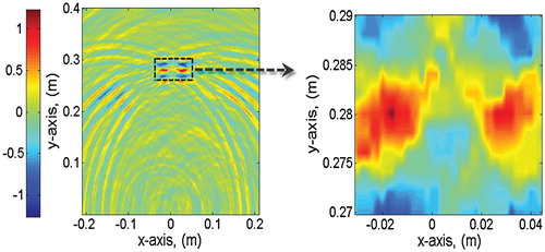
The distance between the two targets drops to 0.4$\lambda$. In that case, by using the conventional TRI, only one target spot exists in the imaging map, the two target cannot be revealed, as shown in Figure 6. Due to the increase of the phase of the signals obtained at points outside the target locations, the time-reversed signals can more focus at the target locations. The imaging map based on the proposed algorithm gives a good idea of the positions of the targets, as shown in Figure 7.

Figure 6. The conventional TRI's imaging results in case 3 at noise free.

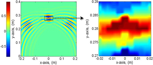
Figure 7. The proposed algorithm's imaging results in case 3 at noise free.

Compared the figures based on the proposed algorithm to those of the conventional TRI, it can be seen that the image pixel values of the proposed algorithm at the target locations are much larger than those of the conventional TRI. It is the result of the multiple time reversal.

The iterative dielectric distribution of the multilayered dielectric slab can help the incident waves create more multiple scattering to carry more information from targets. However, the multilayered dielectric slab has to be close enough to the targets, in order to reach the resolution enhancement. In Liao et al. (2009), when the distance between the multilayered dielectric slab and the targets is 13 cm, it becomes realizable to distinguish the existence of two targets separated by a distance of 18 mm. On the other hand, the proposed algorithm can directly identify the same targets without invoking the multilayered dielectric slab.

Generally speaking, the phase of the time-reversed signals plays the role of assisting the proposed techniques in improving resolution. In conventional TRI theory, the focal characteristic of the time-reversed signals can be enhanced by increasing the physical detection paths. Therefore, the TRIs used to reach high-resolution by means of the high-resolution materials. The proposed algorithm used a different method which optimizes the calculation process. The new calculation method can increase the phase of the time-reversed signal outside the targets. Since the phase is increased, the pixel values outside targets drop more rapidly. Therefore, the resolution can be improved.

For investigating the influence of the noise, the standard white Gaussian noise is added to the echo signals of case 3. The results of the proposed algorithms at SNR = −5 dB and – 10 dB are shown in Figures 8 and 9.

Figure 8. The proposed algorithm's imaging results in case 3 at SNR = −5 dB.

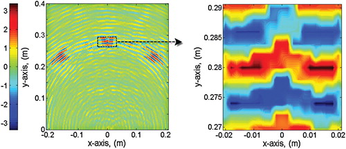
Figure 9. The proposed algorithm's imaging results in case 3 at SNR = −10 dB.

At SNR = −5 dB, the proposed algorithm can suppress the interference of noise and gives a good idea of the target's position. When SNR drops to – 10 dB, the resolution of the left target image gets a little worse. However, the obtained image can still reveal the correct target support clearly, as shown in Figure 8.

The results based on the two methods in case 1 at SNR = −10 dB are shown in Figures 10 and 11. Compared to the results at noise free, the ripple on the imaging maps get more. Furthermore, it can be found that the noise has the same influence on both of the methods.

Figure 10. The proposed algorithm's imaging results in case 1 at SNR = −10 dB.

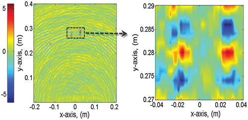
Figure 11. The conventional TRI's imaging results in case 1 at SNR = −10 dB.

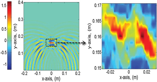
The results with height of the targets = 16 cm, has shown and investigated in this section. Two target points are positioned at (−0.008, 0.16 m) and (0.014, 0.16 m), in order to investigate the influence of the targets’ height. The corresponding imaging results are shown in Figures 12 and 13. With the decrease of the height, the resolution got improved, the conventional TRI can also identified the two targets. However, the sizes of the target images based on the proposed method were till smaller than those of the conventional TRI. That also means the proposed method can improve the resolution.

Figure 12. The proposed algorithm's imaging result with the two target points located at (−0.008, 0.16 m) and (0.014, 0.16 m).

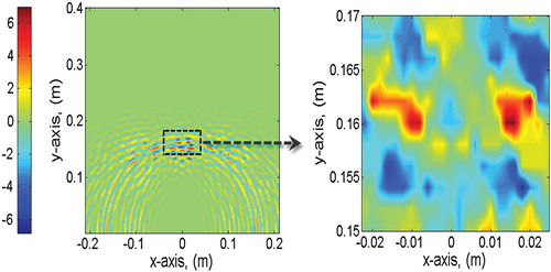
Figure 13. The conventional TRI's imaging result with the two target points located at (−0.008, 0.16 m) and (0.014, 0.16 m).

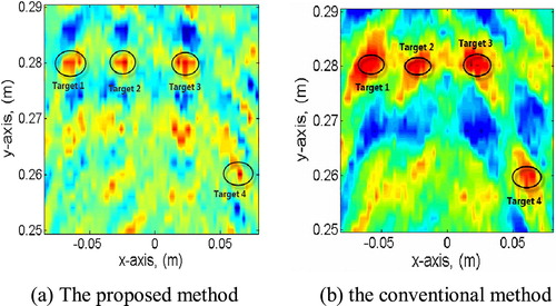
The two methods are used to detect four scatterers whose positions are (−0.06, 0.28 m), (−0.02, 0.28 m), (0.02, 0.28 m) and (0.06, 0.26 m). The results at SNR= −10 dB are shown in Figure 14. The targets can be distinguished from the imaging maps obtained by the both algorithms. The target 1’s image is darker than those of other targets. This difference is caused by the near-problem of the time reversal. The conventional TRI also suffers the same issue. In addition, the noise generates many spurious images in the both results.

Figure 14. The imaging maps based on the two methods in a scene with four scatters at SNR = −10 dB.

4. Measured experiment

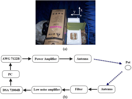
A measured experiment was executed in the following section (Li & Hu, 2015). A cylinder metal pot whose diameter is 15 cm and length is about 25 cm was chosen to be a scatterer in the measured experiment. The cylinder metal pot was centred at (0, 0.295 m), as shown in Figure 15. The Gaussian modulated pulse of 0.2-ns duration centred at 3.5 GHz was used as imaging probe signal, the corresponding frequency band is from 1 to 6 GHz. Seven transceivers were employed to obtain echo signals. The specific positions of the transmitters of all transceivers are respectively (−0.175, 0 m), (−0.125, 0 m), (−0.075, 0 m), (−0.025, 0 m), (0.025, 0 m), (0.075, 0 m) and (0.125, 0 m). The corresponding receivers are located at (−0.225, 0 m), (−0.175, 0 m), (−0.125, 0 m), (−0.075, 0 m), (−0.025, 0 m), (0.025, 0 m) and (0.075, 0 m). During the experiment, the transceivers are realized by one pair of transmit and receive antennas placed at different positions. In each transceiver's location, the probing signal from a Tektronix AWG 7122B arbitrary waveform generator was amplified and transmitted. The echo signal was recorded with Tektronix DSA 72004B.

Figure 15. Experimental set-up. (a) The photo of the measured experiment. (b) The schematic diagram of the measured experiment.

In order to facilitate comparison, all echo signals will be processed by using the proposed method and the conventional TRI method. As shown in Figure 16(a), the target can be distinguished from the imaging maps obtained by the both methods. However, the resolution of the proposed method is much higher than that of the conventional TRI.

Figure 16. Imaging results obtained by using the proposed method and the conventional TRI. (a) The imaging maps. (b) −3 dB width of the target spots.

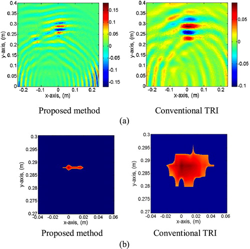
To more clearly show the target's image and investigate the resolution of the proposed algorithm, the −3 dB width of the target spots based on the both algorithms is shown in Figure 16(b). By using the conventional TRI, the −3 dB width of the focal spot is about 6.4 cm × 1.6 cm. On the other hand, due to the temporal–spatial match filtering, the proposed method gives a high resolution of 2.5 cm × 0.25 cm, which represents a significant improvement compares to that of the conventional TRI.

5. Conclusion

Although the high-resolution materials can improve the resolution of the TRIs, they also bring some shortcomings. In this paper, we have exploited the new high-resolution TR imaging algorithm. In the back propagation stage, the proposed algorithm increases the phase of the signals outside the targets by using multiple time reversal operations. Therefore, the proposed algorithm is able to achieve high-resolution without invoking any high-resolution materials. The results show that the resolution of the proposed algorithm outperforms that of the conventional TRI. Since the proposed algorithm can achieve high-resolution without the aid of the high-resolution materials, the proposed algorithm may be a practically valuable approach for high-resolution imaging applications. In future work, the proposed algorithm can be associated with the high-resolution materials, in order to improve resolution furtherly.

Disclosure statement

No potential conflict of interest was reported by the authors.

ORCID

Ning Wang http://orcid.org/0000-0003-1568-6933

Additional information

Funding

This work was partially supported by the Major State Basic Research Development Program of China [973 Program, grant number 2015CB057704] and general project [grant number 51478080] of National Natural Science Foundation of China. The PhD Start-up Fund of Natural Science Foundation of Guangdong Province, China [No. 2014A030310271], Foundation for Distinguished Young Talents in Higher Education of Guangdong, China [No. 2014KQNCX216] and Dongguan Municipal Science and Technology Bureau [grant number 2016508140].

References

- Amitt, E., Dan, G., & Turkel, E. (2014). Time reversal for crack identification. Computational Mechanics, 54, 443–459. doi: 10.1007/s00466-014-0996-2
- Cai, J., Shi, L., & Yuan, S. (2011). High spatial resolution localization for structural health monitoring based on virtual reversal. Smart Materials and Structures, 20, 901–904. doi: 10.1088/0964-1726/20/5/055018
- Fink, M. (1992). Time-reversal of ultrasonic fields – part I: Basic principles. IEEE Transactions on Ultrasonics, Ferroelectrics and Frequency Control, 39(5), 555–566. doi: 10.1109/58.156174
- Fink, M. (1997). Time-reversed acoustics. Scientific American, 281, 91–97. doi: 10.1038/scientificamerican1199-91
- Fouque, J.-P., Garnier, J., Papanicolaou, G., & Sølna, K. (2007). Wave propagation and time reversal in randomly layered media. New York, NY: Springer.
- Gao, Q., Wang, B. Z., & Wang, X. H. (2015). Far-field super-resolution imaging with compact and multifrequency planar resonant lens based on time reversal. IEEE Transactions on Antennas and Propagation, 63(12), 5586–5592. doi: 10.1109/TAP.2015.2496098
- Gao, W., Zhang, G., Li, H., Huo, L., & Song, G. (2017). A novel time reversal sub-group imaging method with noise suppression for damage detection of plate-like structures. Structural Control and Health Monitoring, 25, e2111. doi: 10.1002/stc.2111
- Gong, Z. S., Wang, B. Z., Yang, Y., Zhou, H. C., Ding, S., & Wang, X. H. (2017). Far-field super-resolution imaging of scatterers with a time-reversal system aided by a grating plate. IEEE Photonics Journal, 9(1), 1–8. doi: 10.1109/JPHOT.2016.2640661
- Grbic, A., & Elefteriades, G. V. (2004). Overcoming the diffraction limit with a planar left-handed transmission-line lens. Physical Review Letters, 92, 117403. doi: 10.1103/PhysRevLett.92.117403
- Huo, L., Wang, B., Chen, D., & Song, G. (2017). Monitoring of pre-load on rock bolt using piezoceramic-transducer enabled time reversal method. Sensors, 17, 2467. doi: 10.3390/s17112467
- Ing, R. K., Quieffin, N., Catheline, S., & Fink, M. (2005). In solid localization of finger impacts using acoustic time-reversal process. Applied Physics Letters, 87, 204104. doi: 10.1063/1.2130720
- Kocur, G. K., Vogel, T., & Saenger, E. H. (2011). Crack localization in a double-punched concrete cuboid with time reverse modeling of acoustic emissions. International Journal of Fracture, 171, 1–10. doi: 10.1007/s10704-011-9621-y
- Lemoult, F., Fink, M., & Lerosey, G. (2012). A polychromatic approach to far-field superlensing at visible wavelengths. Nature Communications, 3, 889. doi: 10.1038/ncomms1885
- Lemoult, F., Lerosey, G., de Rosny, J., & Fink, M. (2010). Resonant metalenses for breaking the diffraction barrier. Physical Review Letters, 104(20), 203901. doi: 10.1103/PhysRevLett.104.203901
- Lerosey, G., de Rosny, J., Tourin, A., Derode, A., Montaldo, G., & Fink, M. (2004). Time reversal of electromagnetic waves. Physical Review Letters, 92(19), 193904. doi: 10.1103/PhysRevLett.92.193904
- Li, B., & Hu, B. J. (2015). Time reversal based on noise suppression imaging method by using few echo signals. IEEE Antennas and Wireless Propagation Letters, 14, 12–15. doi: 10.1109/LAWP.2014.2354414
- Liang, Y., Feng, Q., & Li, D. (2018). Loosening monitoring of the threaded pipe connection using time reversal technique and piezoceramic transducers. Sensors, 18, 2280. doi: 10.3390/s18072280
- Liao, T.-H., Hsieh, P.-C., & Chen, F.-C. (2009). Subwavelength target detection using ultrawideband time-reversal techniques with a multilayered dielectric slab. IEEE Antennas and Wireless Propagation Letters, 8, 835–838. doi: 10.1109/LAWP.2009.2025897
- Liu, D., Kang, G., Li, L., & Chen, Y. (2005). Electromagnetic time-reversal imaging of a target in a cluttered environment. IEEE Transactions on Antennas and Propagation, 53, 3058–3066. doi: 10.1109/TAP.2005.854563
- Matthieu, R., Stefan, C., & Philippe, R. (2015). Super-resolution experiments on Lamb waves using a single emitter. Applied Physics Letters, 106, 024103. doi: 10.1063/1.4906105
- Saenger, E. H., Kocur, G. K., Jud, R., & Torrilhon, M. (2011). Application of time reverse modeling on ultrasonic non-destructive testing of concrete. Applied Mathematical Modelling, 35, 807–816. doi: 10.1016/j.apm.2010.07.035
- Shi, G., & Nehorai, A. (2007). A relationship between time-reversal imaging and maximum likelihood scattering estimation. IEEE Transactions on Signal Processing, 55(9), 4707–4711. doi: 10.1109/TSP.2007.896244
- Wang, C. H., Rose, J. T., & Chang, F. K. (2004). A synthetic time-reversal imaging method for structural health monitoring. Smart Materials and Structures, 13, 415–423. doi: 10.1088/0964-1726/13/2/020
- Wang, R., Wang, B. Z., Gong, Z. S., & Ding, X. (2015). Far-field subwavelength imaging with near-field resonant metalens scanning at microwave frequencies. Scientific Reports, 5, 11131. doi: 10.1038/srep11131
- Wu, A., He, S., Ren, Y., Wang, N., Ho, S. C. M., & Song, G. (2019). Design of a new stress wave-based pulse position modulation (PPM) communication system with piezoceramic transducers. Sensors, 19(3), 558. doi: 10.3390/s19030558
- Wu, F., Thomas, J. L., & Fink, M. (1992). Time-reversal of ultrasonic fields – part II: Experimental results. IEEE Transactions on Ultrasonics, Ferroelectrics and Frequency Control, 39(5), 567–578. doi: 10.1109/58.156175
- Yang, Y., Wang, B. Z., & Ding, S. (2018). Performance comparison with different antenna properties in time reversal ultra-wideband communications for sensor system applications. Sensors, 18, 88. doi: 10.3390/s18010088
- Zhang, G., Ho, S. C. M., Huo, L., & Zhu, J. (2019). Negative pressure waves based high resolution leakage localization method using piezoceramic transducers and multiple temporal convolutions. Sensors, 19, 1990. doi: 10.3390/s19091990
- Zhang, G., & Song, Y. (2017a, August). Novel imaging method based on cross-correlation function for suppressing the interference of noise. 2016 IEEE International Conference on Signal and Image Processing, Beijing.
- Zhang, G., & Song, Y. (2017b, August). Time reversal imaging method for damage detection in concrete. 2016 IEEE International Conference on Signal and Image Processing, Beijing.
- Zhang, G., Zhu, J., Song, Y., Peng, C., & Song, G. (2018). A time reversal based pipeline leakage localization method with the Adjustable resolution. IEEE Access, 6, 26993–27000. doi: 10.1109/ACCESS.2018.2829984
- Zhao, G., Zhang, D., Zhang, L., & Wang, B. (2018). Detection of defects in reinforced concrete structures using ultrasonic nondestructive evaluation with piezoceramic transducers and the time reversal method. Sensors, 18, 4176. doi: 10.3390/s18124176