Permanence and Hopf bifurcation of a delayed eco-epidemic model with Leslie–Gower Holling type III functional response

Abstract

This paper is concerned with a delayed eco-epidemic model with a Leslie–Gower Holling type III functional response. The main results are given in terms of permanence and Hopf bifurcation. First of all, sufficient conditions for permanence of the model are established. Directly afterward, sufficient conditions for local stability and existence of Hopf bifurcation are obtained by regarding the delay as bifurcation parameter. Finally, properties of the Hopf bifurcation are investigated with the aid of the normal form theory and centre manifold theorem. Numerical simulations are carried out to verify the obtained theoretical results.

Keywords:

• Eco-epidemic model
• Hopf bifurcation
• permanence
• time delay

1. Introduction

One of the dominant themes in both ecology and mathematical ecology is the dynamic relationship between predators and their preys due to its universal existence and importance in population dynamics (Beretta & Kuang, 1998; Berryman, 1992). As is known, the functional response is an important factor that can affect the dynamical properties of predator–prey systems. During the last decade, many works have been devoted to the study of the effects of a disease on predator–prey systems with different functional responses. In Morozov (2012), Zhang, Jiang, Liu, and Regan (2016), Morozov et al. studied a predator–prey system with disease in the prey and Holling type I functional response. In Hu and Li (2012), Hu and Li investigated the effect of time delay on a predator–prey system with disease in the prey and Holling type I functional response. In Saifuddin, Biswas, Samanta, Sarkar, and Chattopadhyay (2016), Upadhyay and Roy (2014), Sahoo (2015), Saifuddin et al. investigated the eco-epidemiological systems with disease in the prey and Holling type II functional response. Sahoo formulated a predator–prey epidemic model supplying alternative food to predator (Sahoo, 2016). Sahoo assumed that, the interaction between predator and susceptible prey is of Holling type II functional response and that between predator and infected prey is of Holling type I functional response. In Chakraborty, Das, Haldar, and Kar (2015), Chakraborty et al. proposed a predator–prey system with disease in prey and Holling type III functional response based on the work in Bhattacharyya and Mukhopadhyay (2011). Chakraborty et al. studied a ratio-dependent eco-epidemiological system where prey population is subjected to harvesting (Chakraborty, Pal, & Bairagi, 2010). Shi et al. considered an eco-epidemiological model with a stage structure and disease in prey (Shi, Cui, & Zhou, 2011).

In fact, as stated in the literature (Zhang, Li, & Yan,2008), in the predator–prey system, the disease can spread not only in prey but also can spread in predator. Therefore, besides considering the spread of disease in prey, we should also consider the spread of disease in the predator. Based on this consideration, Zhang et al. investigated a delayed predator–prey eco-epidemiological system with disease spreading in predator population and Holling type I functional response (Zhang et al., 2008). Wang et al. formulated a stage-structured predator–prey system with time delay and Holling type II functional response (Wang, Xu, & Feng, 2016). The above eco-epidemiological systems assumed that only the susceptible predator have the ability to capture the prey. As we know, group living is a widespread phenomenon in nature world for animals. Many animals exhibit social behaviour and cooperate with other members of their species in order to improve their skills in defence or hunting. Thus, Hilker et al. proposed an eco-epidemiological model of pack hunting predators that suffer disease infection (Hilker, Paliaga, & Venturino, 2017). Afterwards, Francomano, Hilker, Paliaga, and Venturino (2018) identified the tipping points of the proposed eco-epidemiological model in Hilker et al. (2017).

The Leslie–Gower (LG) formulation is based on the assumption that reduction in a predator population has a reciprocal relationship with per capita availability of its preferred food (Fan, Zhang, & Gao, 2016). This interesting formulation for the predator dynamics has been discussed widely by the scholars at home and abroad (Fan et al., 2016; Gakkhar & Singh, 2012; Nindjin, Tia, & Okou, 2018; Sharma & Samanta, 2015; Wei, Liu, & Zhang, 2018; Xu, Liu, & Yang, 2017; Zhang, Chen, Gao, Fan, & Wang, 2017), and it has been also used in the ecological literature. Recently, Sarwardi et al. proposed an LG Holling type II diseased predator ecosystem in Sarwardi, Haque, and Venturino (2011). However, Holling type II functional response usually suits the invertebral predators. For the vertebral predators, we have to use Holling type III functional response to describe the relationship between the predator and the prey. Based on this consideration, Shaikh, Das, and Ali (2018) investigated a predator–prey system with disease in predator and LG Holling type III functional response.

In general, delay differential equations exhibit much more complicated dynamics than ordinary differential equations since a time delay could cause the population to fluctuate (Wang et al., 2016). Time delays of one type or another have been incorporate into dynamical systems by many researchers (Bairagi & Adak, 2016; Ghosh, Samanta, Biswas, & Rana, 2016; Ghosh et al., 2017; Hu & Li, 2012; Huang, Li, & Cao, 2019; Huang, Nie, et al. 2019; Huang, Zhao, et al. 2019; Li, Huang, & Li, 2019; Li, Wang, Li, Shen, & Lu, 2018; Shi et al., 2011; Wang et al., 2016; Wang, Xie, Lu, & Li, 2019; Xu & Zhang, 2013; Zhang & Wan, 2017; Zhang et al., 2008). Specially, it is well known that periodic solutions can arise through the Hopf bifurcation in delayed dynamical models. Thus, it is interesting to investigate the dynamics of eco-epidemiological systems with time delay. To this end, we study a delayed eco-epidemiological system by incorporating a time delay into system (1(1) $\begin{array}{rl}\frac{\mathrm{d}x\left(t\right)}{\mathrm{d}t}& =a_{1}x\left(t\right)-b_1{x}^2\left(t\right)-\frac{c_1{x}^2\left(t\right)y\left(t\right)}{k_1+x^2\left(t\right)}-\frac{p{c}_1{x}^2\left(t\right)z\left(t\right)}{k_1+x^2\left(t\right)},\\ \frac{\mathrm{d}y\left(t\right)}{\mathrm{d}t}& =a_{2}y\left(t\right)-\frac{c_{2}y\left(t\right)\left(y\right(t)+z(t\left)\right)}{k_2+x\left(t\right)}-\theta y\left(t\right)z\left(t\right),\\ \frac{\mathrm{d}z\left(t\right)}{\mathrm{d}t}& =\theta y\left(t\right)z\left(t\right)+a_{3}z\left(t\right)-\frac{c_{3}z\left(t\right)\left(y\right(t)+z(t\left)\right)}{k_2+x\left(t\right)},\end{array}$(1) ).

The rest of this paper is structured as follows. In Section 2, the delayed eco-epidemic model with LG Holling type III functional response is formulated. In Section 3, permanence of the proposed model is investigated. Sufficient conditions for local stability and existence of Hopf bifurcation are derived in Section 4. Section 5 deals with direction of the Hopf bifurcation, stability and period of the bifurcating periodic solutions. Computer simulations of the model are performed in Section 6. Section 7, which is the last section that contains the conclusions.

2. Model formulation

The proposed eco-epidemic model with LG Holling type III functional response in Shaikh et al. (2018) is as follows (1) $\begin{array}{rl}\frac{\mathrm{d}x\left(t\right)}{\mathrm{d}t}& =a_{1}x\left(t\right)-b_1{x}^2\left(t\right)-\frac{c_1{x}^2\left(t\right)y\left(t\right)}{k_1+x^2\left(t\right)}-\frac{p{c}_1{x}^2\left(t\right)z\left(t\right)}{k_1+x^2\left(t\right)},\\ \frac{\mathrm{d}y\left(t\right)}{\mathrm{d}t}& =a_{2}y\left(t\right)-\frac{c_{2}y\left(t\right)\left(y\right(t)+z(t\left)\right)}{k_2+x\left(t\right)}-\theta y\left(t\right)z\left(t\right),\\ \frac{\mathrm{d}z\left(t\right)}{\mathrm{d}t}& =\theta y\left(t\right)z\left(t\right)+a_{3}z\left(t\right)-\frac{c_{3}z\left(t\right)\left(y\right(t)+z(t\left)\right)}{k_2+x\left(t\right)},\end{array}$(1) where $x\left(t\right)$, $y\left(t\right)$ and $z\left(t\right)$ denote the densities of the prey, the susceptible predator and the infected predator at time t, respectively. $a_1$, $a_2$ and $a_3$ are the intrinsic growth rate of the prey, the susceptible predator and the infected predator, respectively; $b_1$ is the intra-specific competition rate of the prey; $c_1$ is the predation rate of susceptible predator; $c_2$ and $c_3$ are the death rates due to intra-specific competition of the susceptible predator and the infected predator, respectively; θ is the disease incidence rate; $k_1$ is the half saturation constant of the prey; $k_2$ measures the alternative food of the susceptible predator and the infected predator; p is a constant that lies between 0 and 1.

Due to crowding, dynamics of the susceptible predator and the infected predator can be delayed by their negative feedback delay. Time delay can cause a stable equilibrium to become unstable and cause the population to fluctuate, and it can cause interesting dynamics such as bifurcation and periodic solutions. Based on this consideration, we investigate the following delayed eco-epidemic model (2) $\begin{array}{rl}\frac{\mathrm{d}x\left(t\right)}{\mathrm{d}t}& =a_{1}x\left(t\right)-b_1{x}^2\left(t\right)-\frac{c_1{x}^2\left(t\right)y\left(t\right)}{k_1+x^2\left(t\right)}-\frac{p{c}_1{x}^2\left(t\right)z\left(t\right)}{k_1+x^2\left(t\right)},\\ \frac{\mathrm{d}y\left(t\right)}{\mathrm{d}t}& =y\left(t\right)(a_2-\frac{c_2\left(y\right(t-\tau )+z(t-\tau \left)\right)}{k_2+x(t-\tau )}-\theta z\left(t\right)),\\ \frac{\mathrm{d}z\left(t\right)}{\mathrm{d}t}& =z\left(t\right)(\theta y\left(t\right)+a_3-\frac{c_3\left(y\right(t-\tau )+z(t-\tau \left)\right)}{k_2+x(t-\tau )}),\end{array}$(2) subject to the initial condition (3) $\begin{array}{rl}x\left(\alpha \right)& ={\phi }_1\left(\alpha \right)>0,\\ y\left(\alpha \right)& ={\phi }_2\left(\alpha \right)>0,\\ z\left(\alpha \right)& ={\phi }_3\left(\alpha \right)>0,\alpha \in [-\tau ,0),{\phi }_i\left(0\right)>0,i=1,2,3.\end{array}$(3) where τ is the negative feedback delay of the susceptible predator and the infected predator. It should be pointed out that we assume that the feedback delay of the susceptible predator is the same as that of the infected predator throughout the present paper.

3. Permanence

One can check that the system (2(2) $\begin{array}{rl}\frac{\mathrm{d}x\left(t\right)}{\mathrm{d}t}& =a_{1}x\left(t\right)-b_1{x}^2\left(t\right)-\frac{c_1{x}^2\left(t\right)y\left(t\right)}{k_1+x^2\left(t\right)}-\frac{p{c}_1{x}^2\left(t\right)z\left(t\right)}{k_1+x^2\left(t\right)},\\ \frac{\mathrm{d}y\left(t\right)}{\mathrm{d}t}& =y\left(t\right)(a_2-\frac{c_2\left(y\right(t-\tau )+z(t-\tau \left)\right)}{k_2+x(t-\tau )}-\theta z\left(t\right)),\\ \frac{\mathrm{d}z\left(t\right)}{\mathrm{d}t}& =z\left(t\right)(\theta y\left(t\right)+a_3-\frac{c_3\left(y\right(t-\tau )+z(t-\tau \left)\right)}{k_2+x(t-\tau )}),\end{array}$(2) ) has a positive solution with the positive initial condition given in (3(3) $\begin{array}{rl}x\left(\alpha \right)& ={\phi }_1\left(\alpha \right)>0,\\ y\left(\alpha \right)& ={\phi }_2\left(\alpha \right)>0,\\ z\left(\alpha \right)& ={\phi }_3\left(\alpha \right)>0,\alpha \in [-\tau ,0),{\phi }_i\left(0\right)>0,i=1,2,3.\end{array}$(3) ). Now we show that the system (2(2) $\begin{array}{rl}\frac{\mathrm{d}x\left(t\right)}{\mathrm{d}t}& =a_{1}x\left(t\right)-b_1{x}^2\left(t\right)-\frac{c_1{x}^2\left(t\right)y\left(t\right)}{k_1+x^2\left(t\right)}-\frac{p{c}_1{x}^2\left(t\right)z\left(t\right)}{k_1+x^2\left(t\right)},\\ \frac{\mathrm{d}y\left(t\right)}{\mathrm{d}t}& =y\left(t\right)(a_2-\frac{c_2\left(y\right(t-\tau )+z(t-\tau \left)\right)}{k_2+x(t-\tau )}-\theta z\left(t\right)),\\ \frac{\mathrm{d}z\left(t\right)}{\mathrm{d}t}& =z\left(t\right)(\theta y\left(t\right)+a_3-\frac{c_3\left(y\right(t-\tau )+z(t-\tau \left)\right)}{k_2+x(t-\tau )}),\end{array}$(2) ) has permanence. Before proving, we first state the definition of permanence and a lemma which will be used to prove our statement given in Theorem 3.1.

Definition 3.1

see Arino, Wang, & Wolkowicz, 2006; Xia, Kundu, & Maitra, 2018

A system is said to has permanence if for positive constants m and M we have $m\le <\underset{t\to \mathrm{\infty }}{lim}infx\left(t\right)\le \underset{t\to \mathrm{\infty }}{lim}supx\left(t\right)\le M</$ for all positive solutions $x\left(t\right)$ of the system.

Lemma 3.1

see Arino et al., 2006; Xia et al., 2018

If for $t\ge 0$ and $x\left(0\right)\ge 0$ we have $\dot{x}\ge x(c-dx)$ where c>0,d>0 then $\underset{t\to \mathrm{\infty }}{lim}infx\left(t\right)\ge \frac{c}{d}$ and if for $t\ge 0$ and $x\left(0\right)\ge 0$ we have $\dot{x}\le x(c-dx)$ where c>0,d>0 then $\underset{t\to \mathrm{\infty }}{lim}supx\left(t\right)\le \frac{c}{d}.$

Theorem 3.1

Let $M_1,M_2,M_3,m_1,m_2,m_3$ are positive constants and independent of the initial solution of system (2(2) $\begin{array}{rl}\frac{\mathrm{d}x\left(t\right)}{\mathrm{d}t}& =a_{1}x\left(t\right)-b_1{x}^2\left(t\right)-\frac{c_1{x}^2\left(t\right)y\left(t\right)}{k_1+x^2\left(t\right)}-\frac{p{c}_1{x}^2\left(t\right)z\left(t\right)}{k_1+x^2\left(t\right)},\\ \frac{\mathrm{d}y\left(t\right)}{\mathrm{d}t}& =y\left(t\right)(a_2-\frac{c_2\left(y\right(t-\tau )+z(t-\tau \left)\right)}{k_2+x(t-\tau )}-\theta z\left(t\right)),\\ \frac{\mathrm{d}z\left(t\right)}{\mathrm{d}t}& =z\left(t\right)(\theta y\left(t\right)+a_3-\frac{c_3\left(y\right(t-\tau )+z(t-\tau \left)\right)}{k_2+x(t-\tau )}),\end{array}$(2) ), if the following conditions holds

• $m_1\le <\underset{t\to \mathrm{\infty }}{lim}infx\left(t\right)\le \underset{t\to \mathrm{\infty }}{lim}supx\left(t\right)\le M_1$,

• $m_2\le <\underset{t\to \mathrm{\infty }}{lim}infy\left(t\right)\le \underset{t\to \mathrm{\infty }}{lim}supy\left(t\right)\le M_2$,

• $m_3\le <\underset{t\to \mathrm{\infty }}{lim}infz\left(t\right)\le \underset{t\to \mathrm{\infty }}{lim}supz\left(t\right)\le M_3$,

with positive initial condition, i.e. $x\left(0\right)>0,y\left(0\right)>0,z\left(0\right)>0,$ then we say that the system (2(2) $\begin{array}{rl}\frac{\mathrm{d}x\left(t\right)}{\mathrm{d}t}& =a_{1}x\left(t\right)-b_1{x}^2\left(t\right)-\frac{c_1{x}^2\left(t\right)y\left(t\right)}{k_1+x^2\left(t\right)}-\frac{p{c}_1{x}^2\left(t\right)z\left(t\right)}{k_1+x^2\left(t\right)},\\ \frac{\mathrm{d}y\left(t\right)}{\mathrm{d}t}& =y\left(t\right)(a_2-\frac{c_2\left(y\right(t-\tau )+z(t-\tau \left)\right)}{k_2+x(t-\tau )}-\theta z\left(t\right)),\\ \frac{\mathrm{d}z\left(t\right)}{\mathrm{d}t}& =z\left(t\right)(\theta y\left(t\right)+a_3-\frac{c_3\left(y\right(t-\tau )+z(t-\tau \left)\right)}{k_2+x(t-\tau )}),\end{array}$(2) ) has permanence.

Proof.

With the positive initial condition $\left(x\right(0),y(0),z(0\left)\right)$, it is easy to see that the solution $\left(x\right(t),y(t),z(t\left)\right)$ of (2(2) $\begin{array}{rl}\frac{\mathrm{d}x\left(t\right)}{\mathrm{d}t}& =a_{1}x\left(t\right)-b_1{x}^2\left(t\right)-\frac{c_1{x}^2\left(t\right)y\left(t\right)}{k_1+x^2\left(t\right)}-\frac{p{c}_1{x}^2\left(t\right)z\left(t\right)}{k_1+x^2\left(t\right)},\\ \frac{\mathrm{d}y\left(t\right)}{\mathrm{d}t}& =y\left(t\right)(a_2-\frac{c_2\left(y\right(t-\tau )+z(t-\tau \left)\right)}{k_2+x(t-\tau )}-\theta z\left(t\right)),\\ \frac{\mathrm{d}z\left(t\right)}{\mathrm{d}t}& =z\left(t\right)(\theta y\left(t\right)+a_3-\frac{c_3\left(y\right(t-\tau )+z(t-\tau \left)\right)}{k_2+x(t-\tau )}),\end{array}$(2) ) is positive. From the first equation of (2(2) $\begin{array}{rl}\frac{\mathrm{d}x\left(t\right)}{\mathrm{d}t}& =a_{1}x\left(t\right)-b_1{x}^2\left(t\right)-\frac{c_1{x}^2\left(t\right)y\left(t\right)}{k_1+x^2\left(t\right)}-\frac{p{c}_1{x}^2\left(t\right)z\left(t\right)}{k_1+x^2\left(t\right)},\\ \frac{\mathrm{d}y\left(t\right)}{\mathrm{d}t}& =y\left(t\right)(a_2-\frac{c_2\left(y\right(t-\tau )+z(t-\tau \left)\right)}{k_2+x(t-\tau )}-\theta z\left(t\right)),\\ \frac{\mathrm{d}z\left(t\right)}{\mathrm{d}t}& =z\left(t\right)(\theta y\left(t\right)+a_3-\frac{c_3\left(y\right(t-\tau )+z(t-\tau \left)\right)}{k_2+x(t-\tau )}),\end{array}$(2) ), we can write (4) $\frac{\mathrm{d}x}{\mathrm{d}t}\le x(a_1-b_{1}x).$(4) Integrating both sides of (4(4) $\frac{\mathrm{d}x}{\mathrm{d}t}\le x(a_1-b_{1}x).$(4) ) within the interval $[0,t]$ and using the Lemma 3.1, we get (5) $\underset{t\to \mathrm{\infty }}{lim}supx\left(t\right)\le \frac{a_1}{b_1},$(5) where $a_1>0,b_1>0$. Let $M_1=a_1/b_1$, then for $ϵ>0$, ∃ a $T_1>0$ s.t. $x\left(t\right)\le M_1+ϵ$, $\mathrm{\forall }t>T_1$.

Second equation of (2(2) $\begin{array}{rl}\frac{\mathrm{d}x\left(t\right)}{\mathrm{d}t}& =a_{1}x\left(t\right)-b_1{x}^2\left(t\right)-\frac{c_1{x}^2\left(t\right)y\left(t\right)}{k_1+x^2\left(t\right)}-\frac{p{c}_1{x}^2\left(t\right)z\left(t\right)}{k_1+x^2\left(t\right)},\\ \frac{\mathrm{d}y\left(t\right)}{\mathrm{d}t}& =y\left(t\right)(a_2-\frac{c_2\left(y\right(t-\tau )+z(t-\tau \left)\right)}{k_2+x(t-\tau )}-\theta z\left(t\right)),\\ \frac{\mathrm{d}z\left(t\right)}{\mathrm{d}t}& =z\left(t\right)(\theta y\left(t\right)+a_3-\frac{c_3\left(y\right(t-\tau )+z(t-\tau \left)\right)}{k_2+x(t-\tau )}),\end{array}$(2) ), we can write (6) $\frac{\mathrm{d}y}{\mathrm{d}t}\le a_{2}y.$(6) Integrating both sides of (6(6) $\frac{\mathrm{d}y}{\mathrm{d}t}\le a_{2}y.$(6) ) within ‘$t-\tau$’ to ‘t’ we get (7) $y(t-\tau )\ge y\left(t\right)e^{-a_2\tau }.$(7) We get (8) $\frac{\mathrm{d}y}{\mathrm{d}t}\le y\left\{a_2-\frac{c_2{e}^{-a_2\tau }}{k_2+M_1}y\right\},$(8) By using Lemma 3.1, we can write (9) $\underset{t\to \mathrm{\infty }}{lim}supy\left(t\right)\le \frac{a_2(k_2+M_1)}{c_2{e}^{-a_2\tau }}.$(9) Let $M_2=a_2(k_2+M_1)/c_2{e}^{-a_2\tau }$, then for $ϵ>0$, ∃ a $T_2>0$ s.t. $y\left(t\right)\le M_2+ϵ$, $\mathrm{\forall }t>T_2$. Now, following the previous steps, the third equation of (2(2) $\begin{array}{rl}\frac{\mathrm{d}x\left(t\right)}{\mathrm{d}t}& =a_{1}x\left(t\right)-b_1{x}^2\left(t\right)-\frac{c_1{x}^2\left(t\right)y\left(t\right)}{k_1+x^2\left(t\right)}-\frac{p{c}_1{x}^2\left(t\right)z\left(t\right)}{k_1+x^2\left(t\right)},\\ \frac{\mathrm{d}y\left(t\right)}{\mathrm{d}t}& =y\left(t\right)(a_2-\frac{c_2\left(y\right(t-\tau )+z(t-\tau \left)\right)}{k_2+x(t-\tau )}-\theta z\left(t\right)),\\ \frac{\mathrm{d}z\left(t\right)}{\mathrm{d}t}& =z\left(t\right)(\theta y\left(t\right)+a_3-\frac{c_3\left(y\right(t-\tau )+z(t-\tau \left)\right)}{k_2+x(t-\tau )}),\end{array}$(2) ) can be written as: (10) $\frac{\mathrm{d}z}{\mathrm{d}t}\le z(a_3+\theta M_2),$(10) and integrating within ‘$t-\tau$’ to ‘t’, we get (11) $z(t-\tau )\ge z{e}^{-(a_3+\theta M_2)\tau }.$(11) Again from third equation of (2(2) $\begin{array}{rl}\frac{\mathrm{d}x\left(t\right)}{\mathrm{d}t}& =a_{1}x\left(t\right)-b_1{x}^2\left(t\right)-\frac{c_1{x}^2\left(t\right)y\left(t\right)}{k_1+x^2\left(t\right)}-\frac{p{c}_1{x}^2\left(t\right)z\left(t\right)}{k_1+x^2\left(t\right)},\\ \frac{\mathrm{d}y\left(t\right)}{\mathrm{d}t}& =y\left(t\right)(a_2-\frac{c_2\left(y\right(t-\tau )+z(t-\tau \left)\right)}{k_2+x(t-\tau )}-\theta z\left(t\right)),\\ \frac{\mathrm{d}z\left(t\right)}{\mathrm{d}t}& =z\left(t\right)(\theta y\left(t\right)+a_3-\frac{c_3\left(y\right(t-\tau )+z(t-\tau \left)\right)}{k_2+x(t-\tau )}),\end{array}$(2) ), we can write (12) $\frac{\mathrm{d}z}{\mathrm{d}t}\le z\left\{a_3-\frac{c_3{e}^{-(a_3+\theta M_2)\tau }}{k_3+M_1}z\right\},$(12) $\therefore$ Using the Lemma 3.1, we get (13) $\underset{t\to \mathrm{\infty }}{lim}supz\left(t\right)\le \frac{a_3(k_3+M_1)}{c_3{e}^{-(a_3+\theta M_2)\tau }}.$(13) Assume $M_3=a_3(k_3+M_1)/c_3{e}^{-(a_3+\theta M_2)\tau }$, then for $ϵ>0$, ∃ a $T_3>0$ s.t. $z\left(t\right)\le M_3+ϵ$, $\mathrm{\forall }t>T_3$.

Again from the first equation of (2(2) $\begin{array}{rl}\frac{\mathrm{d}x\left(t\right)}{\mathrm{d}t}& =a_{1}x\left(t\right)-b_1{x}^2\left(t\right)-\frac{c_1{x}^2\left(t\right)y\left(t\right)}{k_1+x^2\left(t\right)}-\frac{p{c}_1{x}^2\left(t\right)z\left(t\right)}{k_1+x^2\left(t\right)},\\ \frac{\mathrm{d}y\left(t\right)}{\mathrm{d}t}& =y\left(t\right)(a_2-\frac{c_2\left(y\right(t-\tau )+z(t-\tau \left)\right)}{k_2+x(t-\tau )}-\theta z\left(t\right)),\\ \frac{\mathrm{d}z\left(t\right)}{\mathrm{d}t}& =z\left(t\right)(\theta y\left(t\right)+a_3-\frac{c_3\left(y\right(t-\tau )+z(t-\tau \left)\right)}{k_2+x(t-\tau )}),\end{array}$(2) ), we can write (14) $\begin{array}{rl}\frac{\mathrm{d}x}{\mathrm{d}t}& \ge x\left\{\phantom{\frac{c_1(1+p)(M_1+ϵ)(M_2+ϵ)}{k_1+(M_1+ϵ{)}^2}}{a}_1-b_1(M_1+ϵ)\right.\\ & -\left.\frac{c_1(1+p)(M_1+ϵ)(M_2+ϵ)}{k_1+(M_1+ϵ{)}^2}x\right\},\end{array}$(14) and using the Lemma 3.1 we get (15) $\underset{t\to \mathrm{\infty }}{lim}infx\left(t\right)\ge \frac{\{a_1-b_1(M_1+ϵ\left)\right\}\{k_1+(M_1+ϵ{)}^2\left\}\right)}{c_1(1+p)(M_1+ϵ)(M_2+ϵ)}.$(15) Assume $m_1=\frac{\{a_1-b_1(M_1+ϵ\left)\right\}\{k_1+(M_1+ϵ{)}^2\}}{c_1(1+p)(M_1+ϵ)(M_2+ϵ)},$ then for $ϵ>0$, ∃ a $T_1>0$ s.t. $x\left(t\right)\ge m_1+ϵ$, $\mathrm{\forall }t>T_1$.

The second equation of (2(2) $\begin{array}{rl}\frac{\mathrm{d}x\left(t\right)}{\mathrm{d}t}& =a_{1}x\left(t\right)-b_1{x}^2\left(t\right)-\frac{c_1{x}^2\left(t\right)y\left(t\right)}{k_1+x^2\left(t\right)}-\frac{p{c}_1{x}^2\left(t\right)z\left(t\right)}{k_1+x^2\left(t\right)},\\ \frac{\mathrm{d}y\left(t\right)}{\mathrm{d}t}& =y\left(t\right)(a_2-\frac{c_2\left(y\right(t-\tau )+z(t-\tau \left)\right)}{k_2+x(t-\tau )}-\theta z\left(t\right)),\\ \frac{\mathrm{d}z\left(t\right)}{\mathrm{d}t}& =z\left(t\right)(\theta y\left(t\right)+a_3-\frac{c_3\left(y\right(t-\tau )+z(t-\tau \left)\right)}{k_2+x(t-\tau )}),\end{array}$(2) ) can be written as (16) $\frac{\mathrm{d}y}{\mathrm{d}t}=y\left\{a_2-\theta (M_3+ϵ)-\frac{c_2(M_1+M_3+2ϵ)}{k_2+M_1+ϵ}\right\}.$(16) Integrating both sides of (16(16) $\frac{\mathrm{d}y}{\mathrm{d}t}=y\left\{a_2-\theta (M_3+ϵ)-\frac{c_2(M_1+M_3+2ϵ)}{k_2+M_1+ϵ}\right\}.$(16) ) within $[t-\tau ,t]$, we get (17) $\begin{array}{rl}& y(t-\tau )\\ & \ge y\left(t\right)\exp \left[-\tau \left\{a_2-\theta (M_3+ϵ)-\frac{c_2(M_1+M_3+2ϵ)}{k_2+M_1+ϵ}\right\}\right].\end{array}$(17)

$\therefore$ From the second equation of (2(2) $\begin{array}{rl}\frac{\mathrm{d}x\left(t\right)}{\mathrm{d}t}& =a_{1}x\left(t\right)-b_1{x}^2\left(t\right)-\frac{c_1{x}^2\left(t\right)y\left(t\right)}{k_1+x^2\left(t\right)}-\frac{p{c}_1{x}^2\left(t\right)z\left(t\right)}{k_1+x^2\left(t\right)},\\ \frac{\mathrm{d}y\left(t\right)}{\mathrm{d}t}& =y\left(t\right)(a_2-\frac{c_2\left(y\right(t-\tau )+z(t-\tau \left)\right)}{k_2+x(t-\tau )}-\theta z\left(t\right)),\\ \frac{\mathrm{d}z\left(t\right)}{\mathrm{d}t}& =z\left(t\right)(\theta y\left(t\right)+a_3-\frac{c_3\left(y\right(t-\tau )+z(t-\tau \left)\right)}{k_2+x(t-\tau )}),\end{array}$(2) ), we get (18) $\frac{\mathrm{d}y}{\mathrm{d}t}\ge y\left(t\right){\mathrm{\Delta }}_1,$(18) with (19) $\begin{array}{rl}{\mathrm{\Delta }}_1& =\left\{a_2-\theta (M_3+ϵ)-\frac{c_2(M_3+ϵ)}{k_2+M_1+ϵ}\right.\\ & -\frac{c_2}{k_2+M_1+ϵ}\exp \left[-\tau \left\{\phantom{\frac{c_2}{k_2+M_1+ϵ}}{a}_2-\theta (M_3+ϵ)\right.\right.\\ & \left.\left.\left.-\frac{c_2(M_1+M_3+2ϵ)}{k_2+M_1+ϵ}\right\}\right]y\left(t\right)\right\}.\end{array}$(19) Using the Lemma 3.1, we get (20) $\underset{t\to \mathrm{\infty }}{lim}infy\left(t\right)\ge m_2,$(20) where $m_2=\frac{a_2-\theta (M_3+ϵ)-\frac{c_2(M_3+ϵ)}{k_2+M_1+ϵ}}{\frac{c_2}{k_2+M_1+ϵ}\exp [-\tau \{a_2-\theta (M_3+ϵ)-\frac{c_2(M_1+M_3+2ϵ)}{k_2+M_1+ϵ}\left\}\right]},$

then for $ϵ>0$, ∃ a $T_2>0$ s.t. $y\left(t\right)\ge m_2+ϵ$, $\mathrm{\forall }t>T_2$.

Again, from the third equation of (2(2) $\begin{array}{rl}\frac{\mathrm{d}x\left(t\right)}{\mathrm{d}t}& =a_{1}x\left(t\right)-b_1{x}^2\left(t\right)-\frac{c_1{x}^2\left(t\right)y\left(t\right)}{k_1+x^2\left(t\right)}-\frac{p{c}_1{x}^2\left(t\right)z\left(t\right)}{k_1+x^2\left(t\right)},\\ \frac{\mathrm{d}y\left(t\right)}{\mathrm{d}t}& =y\left(t\right)(a_2-\frac{c_2\left(y\right(t-\tau )+z(t-\tau \left)\right)}{k_2+x(t-\tau )}-\theta z\left(t\right)),\\ \frac{\mathrm{d}z\left(t\right)}{\mathrm{d}t}& =z\left(t\right)(\theta y\left(t\right)+a_3-\frac{c_3\left(y\right(t-\tau )+z(t-\tau \left)\right)}{k_2+x(t-\tau )}),\end{array}$(2) ) we get, (21) $\begin{array}{r}\frac{\mathrm{d}z}{\mathrm{d}t}\ge z\left(t\right)\left\{a_3+\theta (M_2+ϵ)-\frac{c_3(M_2+M_3+2ϵ)}{k_2+M_1+ϵ}\right\},\end{array}$(21) Integrating both sides within $[t-\tau ,t]$, we get (22) $\begin{array}{rl}z(t-\tau )& \ge z\left(t\right)\exp \left[-\tau \left\{\phantom{\frac{c_3(M_2+M_3+2ϵ)}{k_2+M_1+ϵ}}{a}_3+\theta (M_2+ϵ)\right.\right.\\ & -\left.\left.\frac{c_3(M_2+M_3+2ϵ)}{k_2+M_1+ϵ}\right\}\right].\end{array}$(22) Thus from the third equation of (2(2) $\begin{array}{rl}\frac{\mathrm{d}x\left(t\right)}{\mathrm{d}t}& =a_{1}x\left(t\right)-b_1{x}^2\left(t\right)-\frac{c_1{x}^2\left(t\right)y\left(t\right)}{k_1+x^2\left(t\right)}-\frac{p{c}_1{x}^2\left(t\right)z\left(t\right)}{k_1+x^2\left(t\right)},\\ \frac{\mathrm{d}y\left(t\right)}{\mathrm{d}t}& =y\left(t\right)(a_2-\frac{c_2\left(y\right(t-\tau )+z(t-\tau \left)\right)}{k_2+x(t-\tau )}-\theta z\left(t\right)),\\ \frac{\mathrm{d}z\left(t\right)}{\mathrm{d}t}& =z\left(t\right)(\theta y\left(t\right)+a_3-\frac{c_3\left(y\right(t-\tau )+z(t-\tau \left)\right)}{k_2+x(t-\tau )}),\end{array}$(2) ) we get, (23) $\frac{\mathrm{d}z}{\mathrm{d}t}\ge z\left(t\right){\mathrm{\Delta }}_2,$(23) with (24) $\begin{array}{rl}{\mathrm{\Delta }}_2& =\left\{a_3+\theta (M_2+ϵ)-\frac{c_3(M_2+ϵ)}{k_2+M_1+ϵ}\right.\\ & -\frac{c_3}{k_2+M_1+ϵ}\exp \left[-\tau \left\{\phantom{\frac{c_3}{k_2+M_1+ϵ}}{a}_3+\theta (M_2+ϵ)\right.\right.\\ & \left.\left.\left.-\frac{c_3(M_2+M_3+2ϵ)}{k_2+M_1+ϵ}\right\}\right]z\left(t\right)\right\}.\end{array}$(24) Hence Lemma 3.1 gives (25) $\underset{t\to \mathrm{\infty }}{lim}infz\left(t\right)\ge m_3,$(25) where $m_3=\frac{a_3+\theta (M_2+ϵ)-\frac{c_3(M_2+ϵ)}{k_2+M_1+ϵ}}{\frac{c_3}{k_2+M_1+ϵ}\exp [-\tau \{a_3+\theta (M_2+ϵ)-\frac{c_3(M_2+M_3+2ϵ)}{k_2+M_1+ϵ}\left\}\right]},$

then for $ϵ>0$, ∃ a $T_3>0$ s.t. $z\left(t\right)\ge m_3+ϵ$, $\mathrm{\forall }t>T_3$.

Now we assume $ϵ\to 0$ and $T=max\{T_1,T_2,T_3\}$ the $\mathrm{\forall }t>T$ we can write from (5(5) $\underset{t\to \mathrm{\infty }}{lim}supx\left(t\right)\le \frac{a_1}{b_1},$(5) ) & (15(15) $\underset{t\to \mathrm{\infty }}{lim}infx\left(t\right)\ge \frac{\{a_1-b_1(M_1+ϵ\left)\right\}\{k_1+(M_1+ϵ{)}^2\left\}\right)}{c_1(1+p)(M_1+ϵ)(M_2+ϵ)}.$(15) ), (9(9) $\underset{t\to \mathrm{\infty }}{lim}supy\left(t\right)\le \frac{a_2(k_2+M_1)}{c_2{e}^{-a_2\tau }}.$(9) ) & (20(20) $\underset{t\to \mathrm{\infty }}{lim}infy\left(t\right)\ge m_2,$(20) ) and (13(13) $\underset{t\to \mathrm{\infty }}{lim}supz\left(t\right)\le \frac{a_3(k_3+M_1)}{c_3{e}^{-(a_3+\theta M_2)\tau }}.$(13) ) & (25(25) $\underset{t\to \mathrm{\infty }}{lim}infz\left(t\right)\ge m_3,$(25) ) (26) $\begin{array}{rl}{m}_1& \le \underset{t\to \mathrm{\infty }}{lim}infx\left(t\right)\le \underset{t\to \mathrm{\infty }}{lim}supx\left(t\right)\le M_1,\end{array}$(26) (27) $\begin{array}{rl}{m}_2& \le \underset{t\to \mathrm{\infty }}{lim}infy\left(t\right)\le \underset{t\to \mathrm{\infty }}{lim}supy\left(t\right)\le M_2,\end{array}$(27) (28) $\begin{array}{rl}{m}_3& \le \underset{t\to \mathrm{\infty }}{lim}infz\left(t\right)\le \underset{t\to \mathrm{\infty }}{lim}supz\left(t\right)\le M_3,\end{array}$(28) with the positive initial condition $x\left(0\right)>0,y\left(0\right)>0,z\left(0\right)>0$. Thus, we conclude that the system (2(2) $\begin{array}{rl}\frac{\mathrm{d}x\left(t\right)}{\mathrm{d}t}& =a_{1}x\left(t\right)-b_1{x}^2\left(t\right)-\frac{c_1{x}^2\left(t\right)y\left(t\right)}{k_1+x^2\left(t\right)}-\frac{p{c}_1{x}^2\left(t\right)z\left(t\right)}{k_1+x^2\left(t\right)},\\ \frac{\mathrm{d}y\left(t\right)}{\mathrm{d}t}& =y\left(t\right)(a_2-\frac{c_2\left(y\right(t-\tau )+z(t-\tau \left)\right)}{k_2+x(t-\tau )}-\theta z\left(t\right)),\\ \frac{\mathrm{d}z\left(t\right)}{\mathrm{d}t}& =z\left(t\right)(\theta y\left(t\right)+a_3-\frac{c_3\left(y\right(t-\tau )+z(t-\tau \left)\right)}{k_2+x(t-\tau )}),\end{array}$(2) ) has permanence.

4. Local stability and existence of Hopf bifurcation

Based on the analysis in Shaikh et al. (2018), we know that system (2(2) $\begin{array}{rl}\frac{\mathrm{d}x\left(t\right)}{\mathrm{d}t}& =a_{1}x\left(t\right)-b_1{x}^2\left(t\right)-\frac{c_1{x}^2\left(t\right)y\left(t\right)}{k_1+x^2\left(t\right)}-\frac{p{c}_1{x}^2\left(t\right)z\left(t\right)}{k_1+x^2\left(t\right)},\\ \frac{\mathrm{d}y\left(t\right)}{\mathrm{d}t}& =y\left(t\right)(a_2-\frac{c_2\left(y\right(t-\tau )+z(t-\tau \left)\right)}{k_2+x(t-\tau )}-\theta z\left(t\right)),\\ \frac{\mathrm{d}z\left(t\right)}{\mathrm{d}t}& =z\left(t\right)(\theta y\left(t\right)+a_3-\frac{c_3\left(y\right(t-\tau )+z(t-\tau \left)\right)}{k_2+x(t-\tau )}),\end{array}$(2) ) has coexistence equilibrium $E_{\ast }(x_{\ast },y_{\ast },z_{\ast })$, where $\begin{array}{rl}{y}_{\ast }& =\frac{-a_3\theta x_{\ast }-a_3{k}_2\theta +a_2{c}_3-a_3{c}_2}{\theta (\theta x_{\ast }+k_2\theta +c_2-c_3)},\\ z_{\ast }& =-\frac{-a_2\theta x_{\ast }-a_2{k}_2\theta +a_2{c}_3-a_3{c}_2}{\theta (\theta x_{\ast }+k_2\theta +c_2-c_3)},\end{array}$ and $x_{\ast }$ is the positive root of the following equation (29) $A_4{x}^4+A_3{x}^3+A_2{x}^2+A_{1}x+A_0=0,$(29) where $\begin{array}{rl}{A}_3& =b_1{k}_2{\theta }^2-a_1{\theta }^2+b_1{c}_2\theta -b_1{c}_3\theta ,\\ A_2& =-a_1{k}_2{\theta }^2+a_2{c}_1\theta p+b_1{k}_1{\theta }^2-a_1{c}_2\theta \\ & +a_1{c}_3\theta -a_3{c}_1\theta ,\\ A_1& =a_2{c}_1{k}_2\theta p+b_1{k}_1{k}_2{\theta }^2-a_1{k}_1{\theta }^2-a_2{c}_1{c}_{3}p\\ & +a_3{c}_1{c}_{2}p\theta +b_1{c}_2{k}_1\theta -a_3{c}_1{k}_2-b_1{c}_3{k}_1\theta \\ & +a_2{c}_1{c}_3-a_3{c}_1{c}_2,\\ A_0& =-a_1{k}_1{k}_2{\theta }^2-a_1{c}_2{k}_1\theta +a_1{c}_3{k}_1\theta .\end{array}$ The Jacobi matrix of system (2(2) $\begin{array}{rl}\frac{\mathrm{d}x\left(t\right)}{\mathrm{d}t}& =a_{1}x\left(t\right)-b_1{x}^2\left(t\right)-\frac{c_1{x}^2\left(t\right)y\left(t\right)}{k_1+x^2\left(t\right)}-\frac{p{c}_1{x}^2\left(t\right)z\left(t\right)}{k_1+x^2\left(t\right)},\\ \frac{\mathrm{d}y\left(t\right)}{\mathrm{d}t}& =y\left(t\right)(a_2-\frac{c_2\left(y\right(t-\tau )+z(t-\tau \left)\right)}{k_2+x(t-\tau )}-\theta z\left(t\right)),\\ \frac{\mathrm{d}z\left(t\right)}{\mathrm{d}t}& =z\left(t\right)(\theta y\left(t\right)+a_3-\frac{c_3\left(y\right(t-\tau )+z(t-\tau \left)\right)}{k_2+x(t-\tau )}),\end{array}$(2) ) about the coexistence equilibrium $E_{\ast }(x_{\ast },y_{\ast },z_{\ast })$ is given by (30) $J\left(P_{\ast }\right)=\left(\begin{array}{ccc}{m}_{11}& m_{12}& m_{13}\\ n_{21}{e}^{-\lambda \tau }& n_{22}{e}^{-\lambda \tau }& m_{23}+n_{23}{e}^{-\lambda \tau }\\ n_{31}{e}^{-\lambda \tau }& m_{32}+n_{32}{e}^{-\lambda \tau }& n_{33}{e}^{-\lambda \tau }\end{array}\right),$(30) where $\begin{array}{rl}{m}_{11}& =a_1-2b_1{x}_{\ast }-\frac{2c_1{x}_{\ast }{y}_{\ast }}{x_{\ast }^2+k_1}+\frac{2c_1{x}_{\ast }^3{y}_{\ast }}{(x_{\ast }^2+k_1{)}^2}\\ & -\frac{2p{c}_1{x}_{\ast }{z}_{\ast }}{x_{\ast }^2+k_1}+\frac{2p{c}_1{x}_{\ast }^3{z}_{\ast }}{(x_{\ast }^2+k_1{)}^2},\\ m_{12}& =-\frac{c_1{x}_{\ast }^2}{x_{\ast }^2+k_1},m_{13}=-\frac{p{c}_1{x}_{\ast }^2}{x_{\ast }^2+k_1},\\ m_{23}& =-\theta y_{\ast },m_{32}=\theta z_{\ast },\\ n_{21}& =\frac{c_2{y}_{\ast }(y_{\ast }+z_{\ast })}{(x_{\ast }+k_2{)}^2},n_{22}=-\frac{c_2{y}_{\ast }}{x_{\ast }+k_2},\\ n_{23}& =-\frac{c_2{y}_{\ast }}{x_{\ast }+k_2},\\ n_{31}& =\frac{c_3{z}_{\ast }(y_{\ast }+z_{\ast })}{(k_2+x_{\ast }{)}^2},n_{32}=-\frac{c_3{z}_{\ast }}{k_2+x_{\ast }},\\ n_{33}& =-\frac{c_3{z}_{\ast }}{k_2+x_{\ast }}.\end{array}$ The characteristic equation of that matrix (29(29) $A_4{x}^4+A_3{x}^3+A_2{x}^2+A_{1}x+A_0=0,$(29) ) can be obtained as follows: (31) ${\lambda }^3+M_2{\lambda }^2+M_1\lambda +M_0+(N_2{\lambda }^2+N_1\lambda +N_0)e^{-\lambda \tau }=0.$(31) with $\begin{array}{rl}{M}_0& =m_{11}{m}_{23}{m}_{32},M_1=-m_{23}{m}_{32}{M}_2=-m_{11},\\ N_0& =m_{11}(m_{23}{n}_{32}+m_{32}{n}_{23})-m_{12}{m}_{23}{n}_{31}\\ & -m_{13}{m}_{32}{n}_{21},\\ N_1& =m_{11}(n_{22}+n_{33})-m_{12}{n}_{21}-m_{13}{n}_{31}\\ & -m_{32}(n_{23}+n_{32}),\\ N_2& =-(n_{22}+n_{33}).\end{array}$ In order to give the main results in this section, we make some assumptions as follows:

Assumption 4.1

$M_0+N_0>0$, $M_2+N_2>0$, $(M_1+N_1)(M_2+N_2)>M_0+N_0>0$.

Assumption 4.2

(I) $m_0<0$, or (II) $m_0\ge 0$, $m_2^2-3m_1>0$ and $v^{\ast }=(-m_2+\sqrt{m_2^2-3m_1})/3>0$, $f\left(v^{\ast }\right)\le 0$, where $v^{\ast }=(-m_2+\sqrt{m_2^2-3m_1})/3>0$, $f\left(v\right)=v^3+m_2{v}^2+m_{1}v+m_0$ and $\begin{array}{rl}{m}_0& =M_0^2-N_0^2,\\ m_1& =M_1^2-2M_0{M}_2-N_1^2+2N_0{N}_2,\\ m_2& =M_2^2-2M_1-N_2^2.\end{array}$

Assumption 4.3

$f^{\mathrm{\prime }}\left(v_0\right)\ne 0$, where $v_0={\omega }_0^2$ and the expression of ${\omega }_0$ is in the following of this section.

Theorem 4.1

For system (2(2) $\begin{array}{rl}\frac{\mathrm{d}x\left(t\right)}{\mathrm{d}t}& =a_{1}x\left(t\right)-b_1{x}^2\left(t\right)-\frac{c_1{x}^2\left(t\right)y\left(t\right)}{k_1+x^2\left(t\right)}-\frac{p{c}_1{x}^2\left(t\right)z\left(t\right)}{k_1+x^2\left(t\right)},\\ \frac{\mathrm{d}y\left(t\right)}{\mathrm{d}t}& =y\left(t\right)(a_2-\frac{c_2\left(y\right(t-\tau )+z(t-\tau \left)\right)}{k_2+x(t-\tau )}-\theta z\left(t\right)),\\ \frac{\mathrm{d}z\left(t\right)}{\mathrm{d}t}& =z\left(t\right)(\theta y\left(t\right)+a_3-\frac{c_3\left(y\right(t-\tau )+z(t-\tau \left)\right)}{k_2+x(t-\tau )}),\end{array}$(2) ), under Assumptions 4.1–4.3, coexistence equilibrium $E_{\ast }(x_{\ast },y_{\ast },z_{\ast })$ is locally asymptotically stable when $\tau \in [0,{\tau }_0);$ system (2(2) $\begin{array}{rl}\frac{\mathrm{d}x\left(t\right)}{\mathrm{d}t}& =a_{1}x\left(t\right)-b_1{x}^2\left(t\right)-\frac{c_1{x}^2\left(t\right)y\left(t\right)}{k_1+x^2\left(t\right)}-\frac{p{c}_1{x}^2\left(t\right)z\left(t\right)}{k_1+x^2\left(t\right)},\\ \frac{\mathrm{d}y\left(t\right)}{\mathrm{d}t}& =y\left(t\right)(a_2-\frac{c_2\left(y\right(t-\tau )+z(t-\tau \left)\right)}{k_2+x(t-\tau )}-\theta z\left(t\right)),\\ \frac{\mathrm{d}z\left(t\right)}{\mathrm{d}t}& =z\left(t\right)(\theta y\left(t\right)+a_3-\frac{c_3\left(y\right(t-\tau )+z(t-\tau \left)\right)}{k_2+x(t-\tau )}),\end{array}$(2) ) undergoes a Hopf bifurcation at $E_{\ast }(x_{\ast },y_{\ast },z_{\ast })$ when $\tau ={\tau }_0$.

Proof.

When $\tau =0$, Equation (31(31) ${\lambda }^3+M_2{\lambda }^2+M_1\lambda +M_0+(N_2{\lambda }^2+N_1\lambda +N_0)e^{-\lambda \tau }=0.$(31) ) becomes (32) ${\lambda }^3+(M_2+N_2){\lambda }^2+(M_1+N_1)\lambda +M_0+N_0=0.$(32)

Lemma 4.1

Shaikh et al., 2018

The coexistence equilibrium $E_{\ast }(x_{\ast },y_{\ast },z_{\ast })$ is locally asymptotically stable when $\tau =0$ under the Assumption 4.1.

For $\tau >0$, let $\lambda =i\omega (\omega >0)$ be the root of Equation(32(32) ${\lambda }^3+(M_2+N_2){\lambda }^2+(M_1+N_1)\lambda +M_0+N_0=0.$(32) ). We substitute it into Equation (31(31) ${\lambda }^3+M_2{\lambda }^2+M_1\lambda +M_0+(N_2{\lambda }^2+N_1\lambda +N_0)e^{-\lambda \tau }=0.$(31) ). After separating the real and imaginary parts, we have $\begin{array}{rl}& N_1\omega \sin \tau \omega +(N_0-N_2{\omega }^2)\cos \tau \omega =M_2{\omega }^2-M_0,\\ & N_1\omega \cos \tau \omega -(N_0-N_2{\omega }^2)\sin \tau \omega ={\omega }^3-M_1\omega .\end{array}$ Thus we can get the equation with respect to ω (33) ${\omega }^6+m_2{\omega }^4+m_1{\omega }^2+m_0=0,$(33) Let $v={\omega }^2$, then Equation (33(33) ${\omega }^6+m_2{\omega }^4+m_1{\omega }^2+m_0=0,$(33) ) becomes (34) $v^3+m_2{v}^2+m_{1}v+m_0=0.$(34) Define (35) $f\left(v\right)=v^3+m_2{v}^2+m_{1}v+m_0.$(35) If $m_0<0$, then Equation (35(35) $f\left(v\right)=v^3+m_2{v}^2+m_{1}v+m_0.$(35) ) has at least one positive root. On the other hand, if $m_0\ge 0$, based on the Lemma 2.2 in Meng, Huo, Zhang, and Xiang (2011), Equation (35(35) $f\left(v\right)=v^3+m_2{v}^2+m_{1}v+m_0.$(35) ) has positive roots if $m_2^2-3m_1>0$ and $v^{\ast }=(-m_2+\sqrt{m_2^2-3m_1})/3>0$, $f\left(v^{\ast }\right)\le 0$ hold.

Thus, under the Assumption 4.2, Equation (33(33) ${\omega }^6+m_2{\omega }^4+m_1{\omega }^2+m_0=0,$(33) ) has a positive root ${\omega }_0=\sqrt{v_0}$ and Equation (32(32) ${\lambda }^3+(M_2+N_2){\lambda }^2+(M_1+N_1)\lambda +M_0+N_0=0.$(32) ) has a pair of purely imaginary roots $\pm i{\omega }_0$. For ${\omega }_0$, we have ${\tau }_0=\frac{1}{{\omega }_0}\times \arccos \frac{\begin{array}{c}{N}_1{\omega }_0\times ({\omega }_0^3-M_1{\omega }_0)+\\ (N_0-N_2{\omega }_0)\times (M_2{\omega }_0^2-M_0)\end{array}}{N_1^2{\omega }_0^2+(N_0-N_2{\omega }_0^2{)}^2}.$ Differentiating on both sides of Equation (32(32) ${\lambda }^3+(M_2+N_2){\lambda }^2+(M_1+N_1)\lambda +M_0+N_0=0.$(32) ) with respect to τ, we can obtain $[\frac{\mathrm{d}\lambda }{\mathrm{d}\tau }{]}^{-1}=\frac{(3{\lambda }^2+2M_2\lambda +M_1)e^{\lambda \tau }}{\lambda (N_2{\lambda }^2+N_1\lambda +N_0)}-\frac{\tau }{\lambda }.$ Further we have $\mathrm{R}\mathrm{e}[\frac{\mathrm{d}\lambda }{\mathrm{d}\tau }{]}_{\tau ={\tau }_0}^{-1}=\frac{f^{\mathrm{\prime }}\left(v_0\right)}{N_1^2{\omega }_0^2+(N_0-N_2{\omega }_0^2{)}^2},$ where $f\left(v\right)=v^3+m_2{\omega }^2+m_{1}v+m_0$ and $v_0={\omega }_0^2$.

Obviously, under the Assumption 4.3, we know that $\mathrm{R}\mathrm{e}[\mathrm{d}\lambda /\mathrm{d}\tau {]}_{\tau ={\tau }_0}^{-1}\ne 0$. Namely, the transverse condition holds and the conditions for Hopf bifurcation are satisfied at $\tau ={\tau }_0$ according to the Hopf bifurcation theorem in Hassard, Kazarinoff, and Wan (1981). Based on the discussion above and the Hopf bifurcation theorem in Li et al. (2019), we can obtain Theorem 4.1.

5. Properties of Hopf bifurcation

For system (2(2) $\begin{array}{rl}\frac{\mathrm{d}x\left(t\right)}{\mathrm{d}t}& =a_{1}x\left(t\right)-b_1{x}^2\left(t\right)-\frac{c_1{x}^2\left(t\right)y\left(t\right)}{k_1+x^2\left(t\right)}-\frac{p{c}_1{x}^2\left(t\right)z\left(t\right)}{k_1+x^2\left(t\right)},\\ \frac{\mathrm{d}y\left(t\right)}{\mathrm{d}t}& =y\left(t\right)(a_2-\frac{c_2\left(y\right(t-\tau )+z(t-\tau \left)\right)}{k_2+x(t-\tau )}-\theta z\left(t\right)),\\ \frac{\mathrm{d}z\left(t\right)}{\mathrm{d}t}& =z\left(t\right)(\theta y\left(t\right)+a_3-\frac{c_3\left(y\right(t-\tau )+z(t-\tau \left)\right)}{k_2+x(t-\tau )}),\end{array}$(2) ), we have the following results.

Theorem 5.1

If ${\mu }_2>0({\mu }_2<0),$ then the Hopf bifurcation is supercritical (subcritical); If ${\beta }_2<0({\beta }_2>0),$ then the bifurcating periodic solutions are stable (unstable); If $T_2>0(T_2<0),$ then the period of the bifurcating periodic solutions increase (decrease);

and the expressions of ${\mu }_2,{\beta }_2$ and $T_2$ are as follows: (36) $\begin{array}{rl}{C}_1\left(0\right)& =\frac{i}{2{\tau }_0{\omega }_0}(g_{11}{g}_{20}-2|g_{11}{|}^2-\frac{|g_{02}{|}^2}{3})+\frac{g_{21}}{2}\\ {\mu }_2& =-\frac{\mathrm{R}\mathrm{e}\left\{C_1\right(0\left)\right\}}{\mathrm{R}\mathrm{e}\left\{{\lambda }^{\mathrm{\prime }}\right({\tau }_0\left)\right\}},\\ {\beta }_2& =2\mathrm{R}\mathrm{e}\left\{C_1\right(0\left)\right\},\\ T_2& =-\frac{\mathrm{I}\mathrm{m}\left\{C_1\right(0\left)\right\}+{\mu }_2\mathrm{I}\mathrm{m}\left\{{\lambda }^{\mathrm{\prime }}\right({\tau }_0\left)\right\}}{{\tau }_0{\omega }_0},\end{array}$(36)

Proof.

Let $\tau ={\tau }_0+\mu ,\mu \in R$, so that $\mu =0$ is the Hopf bifurcation value for the system. Define the space of continuous real valued functions as $C=C\left(\right[-1,0],R^3)$. Let $u_1\left(t\right)=x\left(t\right)-x_{\ast }$, $u_2\left(t\right)=y\left(t\right)-y_{\ast }$, $u_3\left(t\right)=z\left(t\right)-z_{\ast }$, and normalize time delay with the scaling $t\to \left(t/\tau \right)$. Then, the delay system (2(2) $\begin{array}{rl}\frac{\mathrm{d}x\left(t\right)}{\mathrm{d}t}& =a_{1}x\left(t\right)-b_1{x}^2\left(t\right)-\frac{c_1{x}^2\left(t\right)y\left(t\right)}{k_1+x^2\left(t\right)}-\frac{p{c}_1{x}^2\left(t\right)z\left(t\right)}{k_1+x^2\left(t\right)},\\ \frac{\mathrm{d}y\left(t\right)}{\mathrm{d}t}& =y\left(t\right)(a_2-\frac{c_2\left(y\right(t-\tau )+z(t-\tau \left)\right)}{k_2+x(t-\tau )}-\theta z\left(t\right)),\\ \frac{\mathrm{d}z\left(t\right)}{\mathrm{d}t}& =z\left(t\right)(\theta y\left(t\right)+a_3-\frac{c_3\left(y\right(t-\tau )+z(t-\tau \left)\right)}{k_2+x(t-\tau )}),\end{array}$(2) ) can be transformed into the functional differential equation in C as (37) $\dot{u}\left(t\right)=L_{\mu }\left(u_t\right)+F(\mu ,u_t),$(37) where $u\left(t\right)=(u_1,u_2,u_3{)}^T\in C=C([-1,0],R^3)$ and $L_{\mu }$: $C\to R^3$ and F: $R\times C\to R^3$ are given as follows: $L_{\mu }\phi =({\tau }_0+\mu )\left(A_{max}\phi \right(0)+B_{max}\phi (-1\left)\right),$ and $F(\mu ,\phi )=({\tau }_0+\mu )(F_1,F_2,F_3{)}^T$ with $\begin{array}{rl}{M}_{max}& =\left(\begin{array}{ccc}{m}_{11}& m_{12}& m_{13}\\ 0& 0& m_{23}\\ 0& m_{32}& 0\end{array}\right),\\ N_{max}& =\left(\begin{array}{ccc}0& 0& 0\\ n_{21}& n_{22}& 0\\ n_{31}& n_{32}& n_{33}\end{array}\right).\end{array}$ and $\begin{array}{rl}{F}_1& =g_1{\phi }_1^2\left(0\right)+g_2{\phi }_1\left(0\right){\phi }_2\left(0\right)+g_3{\phi }_1\left(0\right){\phi }_3\left(0\right)\\ & +g_4{\phi }_1^3\left(0\right)+g_5{\phi }_1^2\left(0\right){\phi }_2\left(0\right)\\ & +g_6{\phi }_1^2\left(0\right){\phi }_3\left(0\right)+\cdots ,\\ F_2& =h_1{\phi }_2\left(0\right){\phi }_3\left(0\right)+h_2{\phi }_1(-1){\phi }_2\left(0\right)+h_3{\phi }_1^2(-1)\\ & +h_4{\phi }_1(-1){\phi }_2(-1)\\ & +h_5{\phi }_1(-1){\phi }_3(-1)+h_6{\phi }_2\left(0\right){\phi }_2(-1)\\ & +h_7{\phi }_2\left(0\right){\phi }_3(-1)\\ & +h_8{\phi }_1^3(-1)+h_9{\phi }_1^2(-1){\phi }_2\left(0\right)\\ & +h_{10}{\phi }_1^2(-1){\phi }_2(-1)+h_{11}{\phi }_1^2(-1){\phi }_3(-1)\\ & +h_{12}{\phi }_1(-1){\phi }_2\left(0\right){\phi }_2(-1)\\ & +h_{13}{\phi }_1(-1){\phi }_2\left(0\right){\phi }_3(-1)+\cdots ,\\ F_3& =l_1{\phi }_2\left(0\right){\phi }_3\left(0\right)+l_2{\phi }_1^2(-1)+l_3{\phi }_1(-1){\phi }_3\left(0\right)\\ & +l_4{\phi }_1(-1){\phi }_2(-1)+l_5{\phi }_1(-1){\phi }_3(-1)\\ & +l_6{\phi }_2(-1){\phi }_3\left(0\right)+l_7{\phi }_3\left(0\right){\phi }_3(-1)\\ & +l_8{\phi }_1^3(-1)+l_9{\phi }_1^2(-1){\phi }_3\left(0\right)+l_{10}{\phi }_1^2(-1){\phi }_2(-1)\\ & +l_{11}{\phi }_1^2(-1){\phi }_3(-1)+l_{12}{\phi }_1(-1){\phi }_3\left(0\right){\phi }_3(-1)\\ & +l_{13}{\phi }_1(-1){\phi }_2(-1){\phi }_3\left(0\right),\end{array}$ where $\begin{array}{rl}{g}_1& =-b_1+\frac{c_1{k}_1{x}_{\ast }^2(y_{\ast }+p{z}_{\ast })(3x_{\ast }^2-k_1)}{(x_{\ast }^2+k_1{)}^3},\\ g_2& =-\frac{c_1{k}_1{x}_{\ast }}{(x_{\ast }^2+k_1{)}^2},g_3=-\frac{p{c}_1{k}_1{x}_{\ast }}{(x_{\ast }^2+k_1{)}^2},\\ g_4& =\frac{2c_1{k}_1{x}_{\ast }(y_{\ast }+p{z}_{\ast })}{3(x_{\ast }^2+k_1{)}^3}[k_1-\frac{6x_{\ast }^2(3x_{\ast }^2-k_1)}{x_{\ast }+k_1}],\\ g_5& =\frac{c_1{k}_1(3x_{\ast }^2-k_1)}{(x_{\ast }^2+k_1{)}^3},g_6=\frac{c_1{k}_{1}p(3x_{\ast }^2-k_1)}{(x_{\ast }^2+k_1{)}^3},\\ h_1& =-\theta ,h_2=\frac{c_2(y_{\ast }+z_{\ast })}{(x_{\ast }+k_2{)}^2},h_3=-\frac{c_2{y}_{\ast }(y_{\ast }+z_{\ast })}{(x_{\ast }+k_2{)}^3},\\ h_4& =\frac{c_2{y}_{\ast }}{(x_{\ast }+k_2{)}^2},h_5=\frac{c_2{y}_{\ast }}{(x_{\ast }+k_2{)}^2},h_6=-\frac{c_2}{x_{\ast }+k_2},\\ h_7& =-\frac{c_2}{x_{\ast }+k_2},h_8=\frac{c_2{y}_{\ast }(y_{\ast }+z_{\ast })}{(x+k_2{)}^3},\\ h_9& =-\frac{c_2(y_{\ast }+z_{\ast })}{(x_{\ast }+k_2{)}^3},h_{10}=-\frac{c_2{y}_{\ast }}{(x_{\ast }+k_2{)}^3},\\ h_{11}& =-\frac{c_2{y}_{\ast }}{(x_{\ast }+k_2{)}^3},h_{12}=\frac{c_2}{(x_{\ast }+k_2{)}^2},\\ h_{13}& =\frac{c_2}{(x_{\ast }+k_2{)}^2},l_1=\theta ,l_2=-\frac{c_3{z}_{\ast }(y_{\ast }+z_{\ast })}{x_{\ast }+k_2},\\ l_3& =\frac{c_3(y_{\ast }+z_{\ast })}{(x_{\ast }+k_2{)}^2},l_4=\frac{c_3{z}_{\ast }}{(x_{\ast }+k_2{)}^2},l_5=\frac{c_3{z}_{\ast }}{(x_{\ast }+k_2{)}^2},\\ l_6& =-\frac{c_3}{x_{\ast }+k_2},l_7=\frac{c_3}{x_{\ast }+k_2},l_8=\frac{c_3{z}_{\ast }(y_{\ast }+z_{\ast })}{(x_{\ast }+k_2{)}^4},\\ l_9& =-\frac{c_3(y_{\ast }+z_{\ast })}{(x_{\ast }+k_2{)}^3},l_{10}=-\frac{c_3{z}_{\ast }}{(x_{\ast }+k_2{)}^3},\\ l_{11}& =-\frac{c_3{z}_{\ast }}{(x_{\ast }+k_2{)}^3},l_{12}=\frac{c_3}{(x_{\ast }+k_2{)}^2},\\ l_{13}& =\frac{c_3}{(x_{\ast }+k_2{)}^2}.\end{array}$ According to the Riesz Representation theorem, there exists $\eta (\theta ,{\mu }_0)$ for $\theta \in [-1,0]$ such that (38) $L_{\mu }\phi ={\int }_{-1}^0\mathrm{d}\eta (\theta ,\mu )\phi \left(\theta \right),$(38) for $\phi \in C$. Choosing $\eta (\theta ,\mu )=({\tau }_0+\mu )\left(M_{max}\delta \right(\theta )+N_{max}\delta (\theta +1\left)\right),$ where $\delta \left(\theta \right)$ is the Dirac delta function.

For $\phi \in C\left(\right[-1,0],R^3)$, define $A\left({\mu }_0\right)\phi =\left\{\begin{array}{ll}\frac{\mathrm{d}\phi \left(\theta \right)}{\mathrm{d}\theta },& -1\le \theta <0,\\ {\int }_{-1}^0\mathrm{d}\eta (\theta ,{\mu }_0)\phi \left(\theta \right),& \theta =0,\end{array}\right.$ and $R\left(\mu \right)\phi =\left\{\begin{array}{ll}0,& -1\le \theta <0,\\ F({\mu }_0,\phi ),& \theta =0.\end{array}\right.$ Then, system (37(37) $\dot{u}\left(t\right)=L_{\mu }\left(u_t\right)+F(\mu ,u_t),$(37) ) can be transformed into the following form (39) $\dot{u}\left(t\right)=A\left(\mu \right)u_t+R\left(\mu \right)u_t.$(39) For $\varphi \in C^1\left(\right[0,1],(R^3{)}^{\ast })$, the adjoint operator $A^{\ast }$ of $A\left(0\right)$ is defined as following $A^{\ast }\left(\varphi \right)=\left\{\begin{array}{ll}-\frac{\mathrm{d}\varphi \left(s\right)}{\mathrm{d}s},& 0<s\le 1,\\ {\int }_{-1}^0\mathrm{d}{\eta }^T(s,0)\varphi (-s),& s=0,\end{array}\right.$ Define the bilinear inner form for A and $A^{\ast }$ (40) $\begin{array}{rl}& ⟨\varphi \left(s\right),\phi \left(\theta \right)⟩\\ & =\overline{\varphi }\left(0\right)\phi \left(0\right)-{\int }_{\theta =-1}^0{\int }_{\xi =0}^{\theta }\overline{\varphi }(\xi -\theta )\mathrm{d}\eta \left(\theta \right)\phi \left(\xi \right)\mathrm{d}\xi ,\end{array}$(40) where $\eta \left(\theta \right)=\eta (\theta ,0)$.

Let $\rho \left(\theta \right)=(1,{\rho }_1,{\rho }_2{)}^T{e}^{i{\omega }_0{\tau }_0\theta }$ be the eigenvector of $A\left(0\right)$ corresponding to $+i{\omega }_0{\tau }_0$ and ${\rho }^{\ast }\left(s\right)=D(1,{\rho }_2^{\ast },{\rho }_3^{\ast }{)}^T{e}^{i{\tau }_0{\omega }_{0}s}$ be the eigenvector of $A^{\ast }\left(0\right)$ corresponding to $-i{\tau }_0{\omega }_0$. Then, we can obtain $\begin{array}{rl}{\rho }_2& =\frac{m_{13}{n}_{21}{e}^{-i{\tau }_0{\omega }_0}+m_{23}(i{\omega }_0-m_{11})}{m_{12}{m}_{23}+m_{13}(i{\omega }_0-n_{22}{e}^{-i{\tau }_0{\omega }_0})},\\ {\rho }_3& =\frac{i{\omega }_0-m_{11}-m_{12}{\rho }_2}{m_{13}},\\ {\rho }_2^{\ast }& =-\frac{i{\omega }_0+m_{11}+n_{31}{e}^{i{\tau }_0{\omega }_1}{\rho }_3}{n_{21}{e}^{i{\tau }_0{\omega }_0}},\\ {\rho }_3^{\ast }& =\frac{m_{23}(i{\omega }_0+m_{11})e^{-i{\tau }_0{\omega }_0}-m_{13}{n}_{21}}{m_{23}{n}_{31}-n_{21}(i{\omega }_0-n_{33}{e}^{i{\tau }_0{\omega }_0})}.\end{array}$ Based on Equation (40(40) $\begin{array}{rl}& ⟨\varphi \left(s\right),\phi \left(\theta \right)⟩\\ & =\overline{\varphi }\left(0\right)\phi \left(0\right)-{\int }_{\theta =-1}^0{\int }_{\xi =0}^{\theta }\overline{\varphi }(\xi -\theta )\mathrm{d}\eta \left(\theta \right)\phi \left(\xi \right)\mathrm{d}\xi ,\end{array}$(40) ), we can obtain $\begin{array}{rl}& ⟨\varphi \left(s\right),\phi \left(\theta \right)⟩\\ & =\overline{\varphi }\left(0\right)\phi \left(0\right)-{\int }_{\theta =-1}^0{\int }_{\xi =0}^{\theta }\overline{\varphi }(\xi -\theta )\mathrm{d}\eta \left(\theta \right)\phi \left(\xi \right)\mathrm{d}\xi \\ & =\overline{D}\left[\phantom{{\int }_{-1}^0}1+{\rho }_2{\rho }_2^{\ast }+{\rho }_3{\overline{\rho }}_3^{\ast }\right.\\ & -\left.{\int }_{-1}^0(1,{\overline{\rho }}_2^{\ast },{\overline{\rho }}_3^{\ast })\theta e^{i{\tau }_0{\omega }_0\theta }\mathrm{d}\eta \left(\theta \right)(1,{\rho }_2,{\rho }_3{)}^T\right]\\ & =\overline{D}[1+{\rho }_2{\rho }_2^{\ast }+{\rho }_3{\overline{\rho }}_3^{\ast }+{\tau }_0{e}^{-i{\tau }_0{\omega }_0}(n_{21}{\overline{\rho }}_2^{\ast }\\ & +n_{31}{\overline{\rho }}_3^{\ast }+{\rho }_2(n_{22}{\overline{\rho }}_2^{\ast }+n_{32}{\overline{\rho }}_3^{\ast })+n_{33}{\rho }_3{\overline{\rho }}_3^{\ast }\left)\right].\end{array}$ Let $⟨{\rho }^{\ast },\rho ⟩=1$, then $\begin{array}{rl}\overline{D}& =[1+{\rho }_2{\rho }_2^{\ast }+{\rho }_3{\overline{\rho }}_3^{\ast }+{\tau }_0{e}^{-i{\tau }_0{\omega }_0}(n_{21}{\overline{\rho }}_2^{\ast }\\ & +n_{31}{\overline{\rho }}_3^{\ast }+{\rho }_2(n_{22}{\overline{\rho }}_2^{\ast }+n_{32}{\overline{\rho }}_3^{\ast })+n_{33}{\rho }_3{\overline{\rho }}_3^{\ast }){]}^{-1}.\end{array}$ such that $⟨{\rho }^{\ast },\overline{\rho }⟩=0$.

In what follows, we use the algorithms in Hassard et al. (1981) and the similar computation process to that in Zhang, Upadhyay, Agrawal, and Datta (2018), Zhao and Bi (2017), Xu (2017), we can obtain $\begin{array}{rl}{g}_{20}& =2\overline{D}{\tau }_0[g_1+g_2{\rho }_2+g_3{\rho }_3+{\overline{\rho }}_2^{\ast }(h_1{\rho }_2{\rho }_3\\ & +h_2{\rho }_2{e}^{-i{\tau }_0{\omega }_0}+h_3{e}^{-2i{\tau }_0{\omega }_0}+h_4{\rho }_2{e}^{-2i{\tau }_0{\omega }_0}\\ & +h_5{\rho }_3{e}^{-2i{\tau }_0{\omega }_0}+h_6{\rho }_2^2{e}^{-i{\tau }_0{\omega }_0}+h_7{\rho }_2{\rho }_3{e}^{-i{\tau }_0{\omega }_0})\\ & +{\overline{\rho }}_3^{\ast }(l_1{\rho }_2{\rho }_3+l_2{e}^{-2i{\tau }_0{\omega }_0}+l_3{\rho }_3{e}^{-i{\tau }_0{\omega }_0}\\ & +l_4{\rho }_2{e}^{-2i{\tau }_0{\omega }_0}+l_5{\rho }_3{e}^{-2i{\tau }_0{\omega }_0}\\ & +l_6{\rho }_2{\rho }_3{e}^{-i{\tau }_0{\omega }_0}+l_7{\rho }_3^2{e}^{-i{\tau }_0{\omega }_0}\left)\right],\\ g_{11}& =\overline{D}{\tau }_0[2g_1+g_2({\overline{\rho }}_2+{\rho }_2)+g_3({\overline{\rho }}_3+{\rho }_3)\\ & +{\overline{\rho }}_2^{\ast }\left(h_1\right({\rho }_2{\overline{\rho }}_3+{\rho }_3{\overline{\rho }}_2)+h_2({\overline{\rho }}_2{e}^{-i{\tau }_0{\omega }_0}+{\rho }_2{e}^{i{\tau }_0{\omega }_0})\\ & +2h_3+h_4({\overline{\rho }}_2+{\rho }_2)+h_5({\overline{\rho }}_3+{\rho }_3)\\ & +h_6{\rho }_2{\overline{\rho }}_2(e^{i{\tau }_0{\omega }_0}+e^{-i{\tau }_0{\omega }_0})\\ & +h_7({\rho }_2{\overline{\rho }}_3{e}^{i{\tau }_0{\omega }_0}+{\overline{\rho }}_2{\rho }_3{e}^{-i{\tau }_0{\omega }_0}))\\ & +{\overline{\rho }}_3^{\ast }\left(l_1\right({\rho }_2{\overline{\rho }}_3+{\rho }_3{\overline{\rho }}_2)+2l_2\\ & +l_3({\overline{\rho }}_3{e}^{-i{\tau }_0{\omega }_0}+{\rho }_3{e}^{i{\tau }_0{\omega }_0})\\ & +l_4({\overline{\rho }}_2+{\rho }_2)+l_5({\overline{\rho }}_3+{\rho }_3)\\ & +l_6({\rho }_2{\overline{\rho }}_3{e}^{-i{\tau }_0{\omega }_0}+{\overline{\rho }}_2{\rho }_3{e}^{i{\tau }_0{\omega }_0})\\ & +l_7{\rho }_3{\overline{\rho }}_3(e^{i{\tau }_0{\omega }_0}+e^{-i{\tau }_0{\omega }_0})\left)\right]\\ g_{02}& =2\overline{D}{\tau }_0[g_1+g_2{\overline{\rho }}_2+g_3{\overline{\rho }}_3+{\overline{\rho }}_2^{\ast }(h_1{\overline{\rho }}_2{\overline{\rho }}_3\\ & +h_2{\overline{\rho }}_2{e}^{i{\tau }_0{\omega }_0}+h_3{e}^{2i{\tau }_0{\omega }_0}+h_4{\overline{\rho }}_2{e}^{2i{\tau }_0{\omega }_0}\end{array}$ $\begin{array}{rl}& +h_5{\overline{\rho }}_3{e}^{2i{\tau }_0{\omega }_0}+h_6{\overline{\rho }}_2^2{e}^{i{\tau }_0{\omega }_0}+h_7{\overline{\rho }}_2{\overline{\rho }}_3{e}^{i{\tau }_0{\omega }_0})\\ & +{\overline{\rho }}_3^{\ast }(l_1{\overline{\rho }}_2{\overline{\rho }}_3+l_2{e}^{2i{\tau }_0{\omega }_0}+l_3{\overline{\rho }}_3{e}^{i{\tau }_0{\omega }_0}\\ & +l_4{\overline{\rho }}_2{e}^{2i{\tau }_0{\omega }_0}+l_5{\overline{\rho }}_3{e}^{2i{\tau }_0{\omega }_0}\\ & +l_6{\overline{\rho }}_2{\overline{\rho }}_3{e}^{i{\tau }_0{\omega }_0}+l_7{\overline{\rho }}_3^2{e}^{i{\tau }_0{\omega }_0}\left)\right],\\ g_{21}& =2\overline{D}{\tau }_0[g_1\left(2W_{11}^{\left(1\right)}\right(0)+W_{20}^{\left(1\right)}(0\left)\right)+g_2(W_{11}^{\left(1\right)}\left(0\right){\rho }_2\\ & +\frac{1}{2}{W}_{20}^{\left(1\right)}\left(0\right){\overline{\rho }}_2+W_{11}^{\left(2\right)}\left(0\right)+\frac{1}{2}{W}_{20}^{\left(2\right)}\left(0\right))\\ & +3g_4+g_5({\overline{\rho }}_2+2{\rho }_2)+g_6({\overline{\rho }}_3+2{\rho }_3)\\ & +{\overline{\rho }}_2^{\ast }(h_1(W_{11}^{\left(2\right)}\left(0\right){\rho }_3+\frac{1}{2}{W}_{20}^{\left(2\right)}\left(0\right){\overline{\rho }}_3+W_{11}^{\left(3\right)}\left(0\right){\rho }_2\\ & +\frac{1}{2}{W}_{20}^{\left(3\right)}\left(0\right){\overline{\rho }}_2)+h_2(W_{11}^{\left(1\right)}(-1){\rho }_2+\frac{1}{2}{W}_{20}^{\left(1\right)}(-1){\overline{\rho }}_2\\ & +W_{11}^{\left(2\right)}\left(0\right)e^{-i{\tau }_0{\omega }_0}+\frac{1}{2}{W}_{20}^{\left(2\right)}\left(0\right)e^{i{\tau }_0{\omega }_0})\\ & +h_3(2W_{11}^{\left(1\right)}(-1)e^{-i{\tau }_0{\omega }_0}+W_{20}^{\left(1\right)}(-1)e^{i{\tau }_0{\omega }_0})\\ & +h_4(W_{11}^{\left(1\right)}(-1){\rho }_2{e}^{-i{\tau }_0{\omega }_0}+\frac{1}{2}{W}_{20}^{\left(1\right)}(-1){\overline{\rho }}_2{e}^{i{\tau }_0{\omega }_0}\\ & +W_{11}^{\left(2\right)}(-1)e^{-i{\tau }_0{\omega }_0}+\frac{1}{2}{W}_{20}^{\left(2\right)}(-1)e^{i{\tau }_0{\omega }_0})\\ & +h_5(W_{11}^{\left(1\right)}(-1){\rho }_3{e}^{-i{\tau }_0{\omega }_0}+\frac{1}{2}{W}_{20}^{\left(1\right)}(-1){\overline{\rho }}_3{e}^{i{\tau }_0{\omega }_0}\\ & +W_{11}^{\left(3\right)}(-1)e^{-i{\tau }_0{\omega }_0}+\frac{1}{2}{W}_{20}^{\left(3\right)}(-1)e^{i{\tau }_0{\omega }_0})\\ & +h_6(W_{11}^{\left(2\right)}\left(0\right){\rho }_2{e}^{-i{\tau }_0{\omega }_0}+\frac{1}{2}{W}_{20}^{\left(2\right)}\left(0\right){\overline{\rho }}_2{e}^{i{\tau }_0{\omega }_0}\\ & +W_{11}^{\left(2\right)}(-1){\rho }_2+\frac{1}{2}{W}_{20}^{\left(2\right)}(-1){\overline{\rho }}_2)\\ & +h_7(W_{11}^{\left(2\right)}\left(0\right){\rho }_3{e}^{i{\tau }_0{\omega }_0}+\frac{1}{2}{W}_{20}^{\left(2\right)}(-1){\overline{\rho }}_3{e}^{i{\tau }_0{\omega }_0}\\ & +W_{11}^{\left(3\right)}(-1){\rho }_2+\frac{1}{2}{W}_{20}^{\left(3\right)}(-1){\overline{\rho }}_2)+3h_8{e}^{-i{\tau }_0{\omega }_0}\end{array}$ $\begin{array}{rl}& +h_9({\overline{\rho }}_2{e}^{-2i{\tau }_0{\omega }_0}+2{\rho }_2)+h_{10}{e}^{-i{\tau }_0{\omega }_0}({\overline{\rho }}_2+2{\rho }_2)\\ & +h_{11}{e}^{-i{\tau }_0{\omega }_0}({\overline{\rho }}_3+2{\rho }_3)+h_{12}({\rho }_2{\overline{\rho }}_2+{\rho }_2^2\\ & +{\rho }_2{\overline{\rho }}_2{e}^{-2i{\tau }_0{\omega }_0})+h_{13}({\rho }_2{\overline{\rho }}_3+{\rho }_2{\rho }_3\\ & +{\rho }_2{\overline{\rho }}_3{e}^{-2i{\tau }_0{\omega }_0}))+{\overline{\rho }}_3^{\ast }(l_1(W_{11}^{\left(2\right)}(0){\rho }_3\\ & +\frac{1}{2}{W}_{20}^{\left(2\right)}\left(0\right){\overline{\rho }}_3+W_{11}^{\left(3\right)}\left(0\right){\rho }_2+\frac{1}{2}{W}_{20}^{\left(3\right)}\left(0\right){\overline{\rho }}_2)\\ & +l_2(2W_{11}^{\left(1\right)}(-1)e^{-i{\tau }_0{\omega }_0}+W_{20}^{\left(1\right)}(-1)e^{i{\tau }_0{\omega }_0})\\ & +l_3(W_{11}^{\left(1\right)}(-1){\rho }_3+\frac{1}{2}{W}_{20}^{\left(1\right)}(-1){\overline{\rho }}_3\\ & +W_{11}^{\left(3\right)}\left(0\right)e^{-i{\tau }_0{\omega }_0}+\frac{1}{2}{W}_{20}^{\left(3\right)}\left(0\right)e^{i{\tau }_0{\omega }_0})\\ & +l_4(W_{11}^{\left(1\right)}(-1){\rho }_2{e}^{-i{\tau }_0{\omega }_0}+\frac{1}{2}{W}_{20}^{\left(1\right)}(-1){\overline{\rho }}_2{e}^{i{\tau }_0{\omega }_0}\\ & +W_{11}^{\left(2\right)}(-1)e^{-i{\tau }_0{\omega }_0}+\frac{1}{2}{W}_{20}^{\left(2\right)}(-1)e^{i{\tau }_0{\omega }_0})\\ & +l_5(W_{11}^{\left(1\right)}(-1){\rho }_3{e}^{-i{\tau }_0{\omega }_0}+\frac{1}{2}{W}_{20}^{\left(1\right)}(-1){\overline{\rho }}_3{e}^{i{\tau }_0{\omega }_0}\\ & +W_{11}^{\left(3\right)}(-1)e^{-i{\tau }_0{\omega }_0}+\frac{1}{2}{W}_{20}^{\left(3\right)}(-1)e^{i{\tau }_0{\omega }_0})\\ & +l_6(W_{11}^{\left(3\right)}\left(0\right){\rho }_2{e}^{-i{\tau }_0{\omega }_0}+\frac{1}{2}{W}_{20}^{\left(3\right)}\left(0\right){\overline{\rho }}_2{e}^{i{\tau }_0{\omega }_0}\\ & +W_{11}^{\left(2\right)}(-1){\rho }_3+\frac{1}{2}{W}_{20}^{\left(2\right)}(-1){\overline{\rho }}_3)\\ & +l_7(W_{11}^{\left(3\right)}\left(0\right){\rho }_3{e}^{i{\tau }_0{\omega }_0}+\frac{1}{2}{W}_{20}^{\left(3\right)}(-1){\overline{\rho }}_3{e}^{i{\tau }_0{\omega }_0}\\ & +W_{11}^{\left(3\right)}(-1){\rho }_3+\frac{1}{2}{W}_{20}^{\left(3\right)}(-1){\overline{\rho }}_3)+3l_8{e}^{-i{\tau }_0{\omega }_0}\\ & +l_9({\overline{\rho }}_3{e}^{-2i{\tau }_0{\omega }_0}+2{\rho }_3)+l_{10}{e}^{-i{\tau }_0{\omega }_0}({\overline{\rho }}_2+2{\rho }_2)\\ & +l_{11}{e}^{-i{\tau }_0{\omega }_0}({\overline{\rho }}_3+2{\rho }_3)+l_{12}({\rho }_3{\overline{\rho }}_3+{\rho }_3^2\\ & +{\rho }_3{\overline{\rho }}_3{e}^{-2i{\tau }_0{\omega }_0})+l_{13}({\rho }_2{\overline{\rho }}_3{e}^{-2i{\tau }_0{\omega }_0}\\ & +{\rho }_2{\rho }_3+{\overline{\rho }}_2{\rho }_3))],\end{array}$ with $\begin{array}{rl}{W}_{20}\left(\theta \right)& =\frac{i{g}_{20}\rho \left(0\right)}{{\tau }_0{\omega }_0}{e}^{i{\tau }_0{\omega }_0\theta }+\frac{i{\overline{g}}_{02}\overline{\rho }\left(0\right)}{3{\tau }_0{\omega }_0}{e}^{-i{\tau }_0{\omega }_0\theta }\\ & +E_1{e}^{2i{\tau }_0{\omega }_0\theta },\\ W_{11}\left(\theta \right)& =-\frac{i{g}_{11}\rho \left(0\right)}{{\tau }_0{\omega }_0}{e}^{i{\tau }_0{\omega }_0\theta }+\frac{i{\overline{g}}_{11}\overline{\rho }\left(0\right)}{{\tau }_0{\omega }_0}{e}^{-i{\tau }_0{\omega }_0\theta }+E_2.\end{array}$$E_1$ and $E_2$ can be obtained by the following two equations $\begin{array}{rl}{E}_1& =2\left(\begin{array}{cc}2i{\omega }_0-m_{11}& -m_{12}\\ -n_{21}{e}^{-2i{\tau }_0{\omega }_0}& 2i{\omega }_0-n_{22}{e}^{-2i{\tau }_0{\omega }_0}\\ -n_{31}{e}^{-2i{\tau }_0{\omega }_0}& -m_{32}-n_{32}{e}^{-2i{\tau }_0{\omega }_0}\end{array}\right.\\ & {\left.\begin{array}{c}-m_{13}\\ -m_{23}\\ 2i{\omega }_0-n_{33}{e}^{-2i{\tau }_0{\omega }_0}\end{array}\right)}^{-1}\times \left(\begin{array}{c}{E}_1^{\left(1\right)}\\ E_1^{\left(2\right)}\\ E_1^{\left(3\right)}\end{array}\right),\\ E_2& =2{\left(\begin{array}{ccc}{m}_{11}& m_{12}& m_{13}\\ n_{21}& n_{22}& m_{23}\\ n_{31}& m_{32}+n_{32}& n_{33}\end{array}\right)}^{-1}\times \left(\begin{array}{c}{E}_2^{\left(1\right)}\\ E_2^{\left(2\right)}\\ E_2^{\left(3\right)}\end{array}\right),\end{array}$ where $\begin{array}{rl}{E}_1^{\left(1\right)}& =g_1+g_2{\rho }_2+g_3{\rho }_3,\\ E_1^{\left(2\right)}& =h_1{\rho }_2{\rho }_3+h_2{\rho }_2{e}^{-i{\tau }_0{\omega }_0}+h_3{e}^{-2i{\tau }_0{\omega }_0}\\ & +h_4{\rho }_2{e}^{-2i{\tau }_0{\omega }_0}+h_5{\rho }_3{e}^{-2i{\tau }_0{\omega }_0}\\ & +h_6{\rho }_2^2{e}^{-i{\tau }_0{\omega }_0}+h_7{\rho }_2{\rho }_3{e}^{-i{\tau }_0{\omega }_0},\\ E_1^{\left(3\right)}& =l_1{\rho }_2{\rho }_3+l_2{e}^{-2i{\tau }_0{\omega }_0}+l_3{\rho }_3{e}^{-i{\tau }_0{\omega }_0}\\ & +l_4{\rho }_2{e}^{-2i{\tau }_0{\omega }_0}+l_5{\rho }_3{e}^{-2i{\tau }_0{\omega }_0}\\ & +l_6{\rho }_2{\rho }_3{e}^{-i{\tau }_0{\omega }_0}+l_7{\rho }_3^2{e}^{-i{\tau }_0{\omega }_0}),\\ E_2^{\left(1\right)}& =2g_1+g_2({\overline{\rho }}_2+{\rho }_2)+g_3({\overline{\rho }}_3+{\rho }_3),\\ E_2^{\left(2\right)}& =h_1({\rho }_2{\overline{\rho }}_3+{\rho }_3{\overline{\rho }}_2)+h_2({\overline{\rho }}_2{e}^{-i{\tau }_0{\omega }_0}+{\rho }_2{e}^{i{\tau }_0{\omega }_0})\\ & +2h_3+h_4({\overline{\rho }}_2+{\rho }_2)+h_5({\overline{\rho }}_3+{\rho }_3)\\ & +h_6{\rho }_2{\overline{\rho }}_2(e^{i{\tau }_0{\omega }_0}+e^{-i{\tau }_0{\omega }_0})\\ & +h_7({\rho }_2{\overline{\rho }}_3{e}^{i{\tau }_0{\omega }_0}+{\overline{\rho }}_2{\rho }_3{e}^{-i{\tau }_0{\omega }_0}),\\ E_2^{\left(3\right)}& =l_1({\rho }_2{\overline{\rho }}_3+{\rho }_3{\overline{\rho }}_2)+2l_2+l_3({\overline{\rho }}_3{e}^{-i{\tau }_0{\omega }_0}+{\rho }_3{e}^{i{\tau }_0{\omega }_0})\\ & +l_4({\overline{\rho }}_2+{\rho }_2)+l_5({\overline{\rho }}_3+{\rho }_3)\\ & +l_6({\rho }_2{\overline{\rho }}_3{e}^{-i{\tau }_0{\omega }_0}+{\overline{\rho }}_2{\rho }_3{e}^{i{\tau }_0{\omega }_0})\\ & +l_7{\rho }_3{\overline{\rho }}_3(e^{i{\tau }_0{\omega }_0}+e^{-i{\tau }_0{\omega }_0}).\end{array}$

Thus, we can obtain the expressions of ${\mu }_2$, ${\beta }_2$ and $T_2$. The proof is completed.

6. Numerical simulation

In this section, we present numerical simulation to illustrate our analytical findings. We choose a set of parameters as follows: $a_1=4.5$, $b_1=0.075$, $c_1=2.8$, $k_1=100$, p=0.047, $a_2=3.8$, $c_2=1.97$, $k_2=160$, $\theta =0.0937$, $a_3=0.005$ and $c_3=1.95$. Then system (2(2) $\begin{array}{rl}\frac{\mathrm{d}x\left(t\right)}{\mathrm{d}t}& =a_{1}x\left(t\right)-b_1{x}^2\left(t\right)-\frac{c_1{x}^2\left(t\right)y\left(t\right)}{k_1+x^2\left(t\right)}-\frac{p{c}_1{x}^2\left(t\right)z\left(t\right)}{k_1+x^2\left(t\right)},\\ \frac{\mathrm{d}y\left(t\right)}{\mathrm{d}t}& =y\left(t\right)(a_2-\frac{c_2\left(y\right(t-\tau )+z(t-\tau \left)\right)}{k_2+x(t-\tau )}-\theta z\left(t\right)),\\ \frac{\mathrm{d}z\left(t\right)}{\mathrm{d}t}& =z\left(t\right)(\theta y\left(t\right)+a_3-\frac{c_3\left(y\right(t-\tau )+z(t-\tau \left)\right)}{k_2+x(t-\tau )}),\end{array}$(2) ) becomes (41) $\begin{array}{rl}\frac{\mathrm{d}x\left(t\right)}{\mathrm{d}t}& =4.5x\left(t\right)-0.075x^2\left(t\right)-\frac{2.8x^2\left(t\right)y\left(t\right)}{100+x^2\left(t\right)}\\ & -\frac{0.1316x^2\left(t\right)z\left(t\right)}{100+x^2\left(t\right)},\\ \frac{\mathrm{d}y\left(t\right)}{\mathrm{d}t}& =y\left(t\right)\left(3.8-\frac{1.97\left(y\right(t-\tau )+z(t-\tau \left)\right)}{160+x(t-\tau )}\right.\\ & -\left.0.0937z\left(t\right)\phantom{\frac{1.97\left(y\right(t-\tau )+z(t-\tau \left)\right)}{160+x(t-\tau )}}\right),\\ \frac{\mathrm{d}z\left(t\right)}{\mathrm{d}t}& =z\left(t\right)\left(\phantom{\frac{1.95\left(y\right(t-\tau )+z(t-\tau \left)\right)}{160+x(t-\tau )}}0.0937y\left(t\right)+0.005\right.\\ & -\left.\frac{1.95\left(y\right(t-\tau )+z(t-\tau \left)\right)}{160+x(t-\tau )}\right).\end{array}$(41) With the aid of Matlab software package, we can obtain the unique coexistence equilibrium $E_{\ast }(56.4348$, $3.8372,36.6245)$ of system (41(41) $\begin{array}{rl}\frac{\mathrm{d}x\left(t\right)}{\mathrm{d}t}& =4.5x\left(t\right)-0.075x^2\left(t\right)-\frac{2.8x^2\left(t\right)y\left(t\right)}{100+x^2\left(t\right)}\\ & -\frac{0.1316x^2\left(t\right)z\left(t\right)}{100+x^2\left(t\right)},\\ \frac{\mathrm{d}y\left(t\right)}{\mathrm{d}t}& =y\left(t\right)\left(3.8-\frac{1.97\left(y\right(t-\tau )+z(t-\tau \left)\right)}{160+x(t-\tau )}\right.\\ & -\left.0.0937z\left(t\right)\phantom{\frac{1.97\left(y\right(t-\tau )+z(t-\tau \left)\right)}{160+x(t-\tau )}}\right),\\ \frac{\mathrm{d}z\left(t\right)}{\mathrm{d}t}& =z\left(t\right)\left(\phantom{\frac{1.95\left(y\right(t-\tau )+z(t-\tau \left)\right)}{160+x(t-\tau )}}0.0937y\left(t\right)+0.005\right.\\ & -\left.\frac{1.95\left(y\right(t-\tau )+z(t-\tau \left)\right)}{160+x(t-\tau )}\right).\end{array}$(41) ) and the conditions of local asymptotic stability of $E_{\ast }$ are satisfied when $\tau =0$. For $\tau >0$, we can obtain ${\omega }_0=0.6049$, ${\tau }_0=1.2015$ and ${\lambda }^{\mathrm{\prime }}\left({\tau }_0\right)=1.4076+0.8266i$. Thus we can derive the following values $C_1\left(0\right)=-3.0818+1.2297i$, ${\mu }_2=2.1894>0$, ${\beta }_2=-6.1636<0$ and $T_2=-4.1820<0$.

Thus, $E_{\ast }(56.4348$, $3.8372,36.6245)$ is locally asymptotically stable when $\tau \in [0,{\tau }_0=1.2015)$, which can be illustrated by Figure 1. As can be seen from Figure 1, fixing $\tau =1.1865\in [0,{\tau }_0=1.2015)$, the solution of system (41(41) $\begin{array}{rl}\frac{\mathrm{d}x\left(t\right)}{\mathrm{d}t}& =4.5x\left(t\right)-0.075x^2\left(t\right)-\frac{2.8x^2\left(t\right)y\left(t\right)}{100+x^2\left(t\right)}\\ & -\frac{0.1316x^2\left(t\right)z\left(t\right)}{100+x^2\left(t\right)},\\ \frac{\mathrm{d}y\left(t\right)}{\mathrm{d}t}& =y\left(t\right)\left(3.8-\frac{1.97\left(y\right(t-\tau )+z(t-\tau \left)\right)}{160+x(t-\tau )}\right.\\ & -\left.0.0937z\left(t\right)\phantom{\frac{1.97\left(y\right(t-\tau )+z(t-\tau \left)\right)}{160+x(t-\tau )}}\right),\\ \frac{\mathrm{d}z\left(t\right)}{\mathrm{d}t}& =z\left(t\right)\left(\phantom{\frac{1.95\left(y\right(t-\tau )+z(t-\tau \left)\right)}{160+x(t-\tau )}}0.0937y\left(t\right)+0.005\right.\\ & -\left.\frac{1.95\left(y\right(t-\tau )+z(t-\tau \left)\right)}{160+x(t-\tau )}\right).\end{array}$(41) ) with initial value $x\left(0\right)=39$, $y\left(0\right)=3.55$ and $z\left(0\right)=29.2745$ would tend to $E_{\ast }(56.4348,3.8372,36.6245)$; that is, $E_{\ast }(56.4348$, $3.8372,36.6245)$ is locally asymptotically stable. However, once the value of τ passes through the critical value ${\tau }_0=1.2015$, the coexistence equilibrium $(56.4348,3.8372,36.6245)$ loses its stability and a Hopf bifurcation occurs; that is, a family of periodic solutions bifurcate from $E_{\ast }(56.4348,3.8372,36.6245)$. 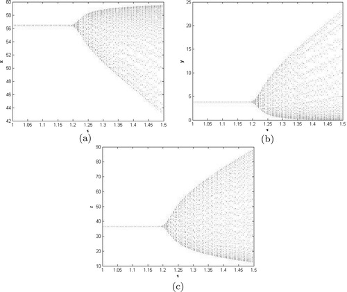This property can be shown as in Figure 2. The bifurcation phenomenon can be also illustrated by the bifurcation diagrams in Figure 3. In addition, since ${\mu }_2>0$, ${\beta }_2<0$ and $T_2<0$, according to Theorem 5.1, we can conclude that the Hopf bifurcation is supercritical; the bifurcating periodic solutions are stable; and the period of the bifurcating periodic solutions decreases.

Figure 1. $E_{\ast }$ is locally asymptotically stable when $\tau =1.1865<{\tau }_0=1.2015$ with initial values ‘39, 3.55, 29.2745’. (a) The trajectory of x, (b) The trajectory of y, (c) The trajectory of z and (d) The phase plot of x, y and z.

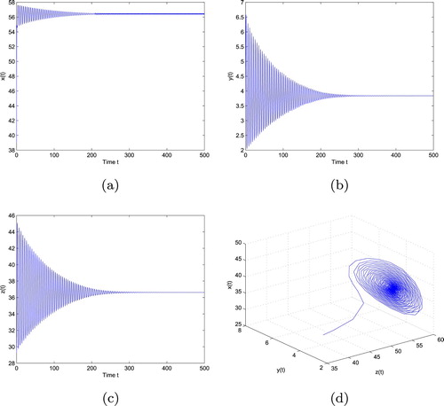
Figure 2. $E_{\ast }$ loses stability and undergoes a Hopf bifurcation when $\tau =1.2295>{\tau }_0=1.2015$ with initial values ‘39, 3.55, 29.2745’. (a) The trajectory of x, (b) The trajectory of y, (c) The trajectory of z and (d) The phase plot of x, y and z.

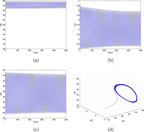
Figure 3. Bifurcation diagram with respect to time delay. (a) Bifurcation diagram of x, (b) Bifurcation diagram of y and (c) Bifurcation diagram of z.

7. Conclusions

In this paper, a delayed eco-epidemic model with LG Holling type III functional response is proposed by incorporating the negative feedback delay of the susceptible predator and the infected predator into the model formulated in the literature (Shaikh et al., 2018). Compared with the work by Shaikh et al. (2018), we mainly focus on the effect of the time delay on the model and the model in the present paper is more general.

It has been shown that, under some conditions, the system (2(2) $\begin{array}{rl}\frac{\mathrm{d}x\left(t\right)}{\mathrm{d}t}& =a_{1}x\left(t\right)-b_1{x}^2\left(t\right)-\frac{c_1{x}^2\left(t\right)y\left(t\right)}{k_1+x^2\left(t\right)}-\frac{p{c}_1{x}^2\left(t\right)z\left(t\right)}{k_1+x^2\left(t\right)},\\ \frac{\mathrm{d}y\left(t\right)}{\mathrm{d}t}& =y\left(t\right)(a_2-\frac{c_2\left(y\right(t-\tau )+z(t-\tau \left)\right)}{k_2+x(t-\tau )}-\theta z\left(t\right)),\\ \frac{\mathrm{d}z\left(t\right)}{\mathrm{d}t}& =z\left(t\right)(\theta y\left(t\right)+a_3-\frac{c_3\left(y\right(t-\tau )+z(t-\tau \left)\right)}{k_2+x(t-\tau )}),\end{array}$(2) ) is permanent. Moreover, we find that the negative feedback delay of the predator may destabilize the coexistence equilibrium of the eco-epidemiological system and cause the population to fluctuate if the given conditions are satisfied. Particularly, there is a threshold ${\tau }_0$ for the time delay such that below it the coexistence equilibrium is locally asymptotically stable. In this case, the disease spreading among the predators can be controlled. However, if the delay is greater than the threshold ${\tau }_0$, a Hopf bifurcation arises. This implies that the disease spreading among the predators becomes periodically endemic and the disease among the predators is out of control. Furthermore, properties of the Hopf bifurcation such as direction and stability are investigated. Finally, we present some numerical simulations to support our theoretical results.

However, we only consider the existence of the local Hopf bifurcation of the system (2(2) $\begin{array}{rl}\frac{\mathrm{d}x\left(t\right)}{\mathrm{d}t}& =a_{1}x\left(t\right)-b_1{x}^2\left(t\right)-\frac{c_1{x}^2\left(t\right)y\left(t\right)}{k_1+x^2\left(t\right)}-\frac{p{c}_1{x}^2\left(t\right)z\left(t\right)}{k_1+x^2\left(t\right)},\\ \frac{\mathrm{d}y\left(t\right)}{\mathrm{d}t}& =y\left(t\right)(a_2-\frac{c_2\left(y\right(t-\tau )+z(t-\tau \left)\right)}{k_2+x(t-\tau )}-\theta z\left(t\right)),\\ \frac{\mathrm{d}z\left(t\right)}{\mathrm{d}t}& =z\left(t\right)(\theta y\left(t\right)+a_3-\frac{c_3\left(y\right(t-\tau )+z(t-\tau \left)\right)}{k_2+x(t-\tau )}),\end{array}$(2) ). We leave the existence of the global Hopf bifurcation for our next work. In addition, we neglect the negative feedback delay of the prey in the system (2(2) $\begin{array}{rl}\frac{\mathrm{d}x\left(t\right)}{\mathrm{d}t}& =a_{1}x\left(t\right)-b_1{x}^2\left(t\right)-\frac{c_1{x}^2\left(t\right)y\left(t\right)}{k_1+x^2\left(t\right)}-\frac{p{c}_1{x}^2\left(t\right)z\left(t\right)}{k_1+x^2\left(t\right)},\\ \frac{\mathrm{d}y\left(t\right)}{\mathrm{d}t}& =y\left(t\right)(a_2-\frac{c_2\left(y\right(t-\tau )+z(t-\tau \left)\right)}{k_2+x(t-\tau )}-\theta z\left(t\right)),\\ \frac{\mathrm{d}z\left(t\right)}{\mathrm{d}t}& =z\left(t\right)(\theta y\left(t\right)+a_3-\frac{c_3\left(y\right(t-\tau )+z(t-\tau \left)\right)}{k_2+x(t-\tau )}),\end{array}$(2) ). Therefore, we will investigate the Hopf bifurcation of the following system with multiple delays by considering the different combinations of the delays as the bifurcation parameter: (42) $\begin{array}{rl}\frac{\mathrm{d}x\left(t\right)}{\mathrm{d}t}& =x\left(t\right)\left(a_1-b_{1}x(t-{\tau }_1)-\frac{c_{1}x\left(t\right)y\left(t\right)}{k_1+x^2\left(t\right)}\right.\\ & -\left.\frac{p{c}_{1}x\left(t\right)z\left(t\right)}{k_1+x^2\left(t\right)}\right),\\ \frac{\mathrm{d}y\left(t\right)}{\mathrm{d}t}& =y\left(t\right)(a_2-\frac{c_2\left(y\right(t-{\tau }_2)+z(t-{\tau }_2\left)\right)}{k_2+x(t-{\tau }_2)}-\theta z\left(t\right)),\\ \frac{\mathrm{d}z\left(t\right)}{\mathrm{d}t}& =z\left(t\right)(\theta y\left(t\right)+a_3-\frac{c_3\left(y\right(t-{\tau }_3)+z(t-{\tau }_3\left)\right)}{k_2+x(t-{\tau }_3)}),\end{array}$(42) where ${\tau }_1$, ${\tau }_2$ and ${\tau }_3$ are the negative feedback delay of the prey, the susceptible predator and the infected predator, respectively.

Acknowledgements

The authors are grateful to the editor and the anonymous referees for their valuable comments and suggestions on the paper.

Disclosure statement

No potential conflict of interest was reported by the authors.

Additional information

Funding

This research was supported by Natural Science Foundation of Anhui Province [grant number 1708085MA17], Project of Support Program for Excellent Youth Talent in Colleges and Universities of Anhui Province [grant numbers gxyqZD2018044, gxbjZD49] and the Natural Science Foundation of the Higher Education Institutions of Anhui Province [grant numbers KJ2018A0437, KJ2019A0655, KJ2019A0662].

References

- Arino, J., Wang, L., & Wolkowicz, G. S. (2006). An alternative formulation for a delayed logistic equation. Journal of Theoretical Biology, 241(1), 109–119.
- Bairagi, N., & Adak, D. (2016). Switching from simple to complex dynamics in a predator-prey-parasite model: An interplay between infection rate and incubation delay. Mathematical Biosciences, 277(7), 1–14.
- Beretta, E., & Kuang, Y. (1998). Global analyses in some delayed ratio-dependent predator-prey systems. Nonlinear Analysis: Theory, Methods and Applications, 32(3), 381–408.
- Berryman, A. A. (1992). The origins and evolution of predator-prey theory. Ecology, 73(5), 1530–1535.
- Bhattacharyya, R., & Mukhopadhyay, B. (2011). On an epidemiological model with nonlinear infection incidence: Local and global perspective. Applied Mathematical Modelling, 35(7), 3166–3174.
- Chakraborty, K., Das, K., Haldar, S., & Kar, T. K. (2015). A mathematical study of an eco-epidemiological system on disease persistence and extinction perspective. Applied Mathematics and Computation, 254(3), 99–112.
- Chakraborty, S., Pal, S., & Bairagi, N. (2010). Dynamics of a ratio-dependent eco-epidemiological system with prey harvesting. Nonlinear Analysis: Real World Applications, 11(3), 1862–1877.
- Fan, K. G., Zhang, Y., & Gao, S. J. (2016). On a new eco-epidemiological model for migratory birds with modified Leslie-Gower functional schemes. Advances in Difference Equations, 97(12), 1–20.
- Francomano, E., Hilker, F. M., Paliaga, M., & Venturino, E. (2018). Separatrix reconstruction to identify tipping points in an eco-epidemiological model. Applied Mathematics and Computation, 318(7), 80–91.
- Gakkhar, S., & Singh, A. (2012). Complex dynamics in a prey predator system with multiple delays. Communications in Nonlinear Science and Numerical Simulation, 17(2), 914–929.
- Ghosh, K., Biswas, S., Samanta, S., Tiwari, P. K., Alshomrani, A. S., & Chattopadhyay, J (2017). Effect of multiple delays in an eco-epidemiological model with strong Allee effect. International Journal of Bifurcation and Chaos, 27(11), 1750167.
- Ghosh, K., Samanta, S., Biswas, S., & Rana, S. (2016). Stability and bifurcation analysis of an eco-epidemiological model with multiple delays. Nonlinear Studies, 23(2), 167–208.
- Hassard, B. D., Kazarinoff, N. D., & Wan, Y. H (1981). Theory and applications of Hopf bifurcation. Cambridge: Cambridge University Press.
- Hilker, F. M., Paliaga, M., & Venturino, E. (2017). Diseased social predators. Bulletin of Mathematical Biology, 79(10), 2175–2196.
- Hu, G. P., & Li, X. L. (2012). Stability and Hopf bifurcation for a delayed predator-prey model with disease in the prey. Chaos, Solitons and Fractals, 45(3), 229–237.
- Huang, C. D., Li, H., & Cao, J. D. (2019). A novel strategy of bifurcation control for a delayed fractional predator-prey model. Applied Mathematics and Computation, 347(4), 808–838.
- Huang, C. D., Nie, X. B., Zhao, X., Song, Q. K., Tu, Z. W., Xiao, M., & Cao, J. D. (2019). Novel bifurcation results for a delayed fractional-order quaternion-valued neural network. Neural Networks, 117(5), 67–93.
- Huang, C. D., Zhao, X., Wang, X. H., Wang, Z. X., Xiao, M., & Cao, J. D. (2019). Disparate delays-induced bifurcations in a fractional-order neural network. Journal of the Franklin Institute, 356(5), 2825–2846.
- Li, H., Huang, C. D., & Li, T. X. (2019). Dynamic complexity of a fractional-order predator-prey system with double delays. Physica A, 526(120852), 1–16.
- Li, L., Wang, Zhen., Li, Y. X., Shen, H., & Lu, J. W. (2018). Hopf bifurcation analysis of a complex-valued neural network model with discrete and distributed delays. Applied Mathematics and Computation, 330(1), 152–169.
- Meng, X. Y., Huo, H. F., Zhang, X. B., & Xiang, H. (2011). Stability and Hopf bifurcation in a three-species system with feedback delays. Nonlinear Dynamics, 64(4), 349–364.
- Morozov, A. Y. (2012). Revealing the role of predator-dependent disease transmission in the epidemiology of a wildlife infection: A model study. Theoretical Ecology, 5(4), 517–532.
- Nindjin, A. F., Tia, K. T., & Okou, H. (2018). Stability of a diffusive predator-prey model with modified Leslie-Gower and Holling-type II schemes and time-delay in two dimensions. Advances in Difference Equations, 177(12), 1–17.
- Sahoo, B. (2015). Role of additional food in eco-epidemiological system with disease in the prey. Applied Mathematics and Computation, 259(5), 61–79.
- Sahoo, B. (2016). Disease control through provision of alternative food to predator: A model based study. International Journal of Dynamics and Control, 4(3), 239–253.
- Saifuddin, M., Biswas, S., Samanta, S., Sarkar, S., & Chattopadhyay, J. (2016). Complex dynamics of an eco-epidemiological model with different competition coefficients and weak Allee in the predator. Chaos, Solitons and Fractals, 91(10), 270–285.
- Sarwardi, S., Haque, M., & Venturino, E. (2011). Global stability and persistence in LG-Holling type II diseased predator ecosystems. Journal of Biological Physics, 37(1), 91–106.
- Shaikh, A. A., Das, H., & Ali, N. (2018). Study of LG-Holling type III predator-prey model with disease in predator. Journal of Applied Mathematics and Computing, 58(2), 235–255.
- Sharma, S., & Samanta, G. P. (2015). A Leslie-Gower predator-prey model with disease in prey incorporating a prey refuge. Chaos Solitons and Fractals, 70(1), 69–84.
- Shi, X. Y., Cui, J. A., & Zhou, X. Y (2011). Stability and Hopf bifurcation analysis of an eco-epidemic model with a stage structure. Nonlinear Analysis, 74(4), 1088-–1106.
- Upadhyay, R. K., & Roy, P. (2014). Spread of a disease and its effect on population dynamics in an eco-epidemiological system. Communications in Nonlinear Science and Numerical Simulation, 19(12), 4170–4184.
- Wang, L. S., Xu, R., & Feng, G. H. (2016). Modelling and analysis of an eco-epidemiological model with time delay and stage structure. Journal of Applied Mathematics and Computing, 50(1–2), 175–197.
- Wang, Z., Xie, Y. K., Lu, J. W., & Li, Y. X. (2019). Stability and bifurcation of a delayed generalized fractional-order prey-predator model with interspecific competition. Applied Mathematics and Computation, 347(2), 360–369.
- Wei, C. J., Liu, J. N., & Zhang, S. W. (2018). Analysis of a stochastic eco-epidemiological model with modified Leslie-Gower functional response. Advances in Difference Equations, 119(12), 1–17.
- Xia, W. J., Kundu, S., & Maitra, S. (2018). Dynamics in dynamics of a delayed SEIQ epidemic model. Advances in Difference Equations, 336(9), 1–21.
- Xu, C. J. (2017). Delay-induced oscillations in a competitor-competitor-mutualist Lotka-Volterra model. Complexity, 2017(4), 1–12.
- Xu, Y., Liu, M., & Yang, Y. (2017). Analysis of a stochastic two-predators one-prey system with modified Leslie-Gower and Holling-type II schemes. Journal of Applied Analysis and Computation, 7(2), 713–727.
- Xu, R., & Zhang, S. H. (2013). Modelling and analysis of a delayed predator-prey model with disease in the predator. Applied Mathematics and Computation, 224(11), 372–386.
- Zhang, Y., Chen, S., Gao, S., Fan, K., & Wang, Q. (2017). A new non-autonomous model for migratory birds with Leslie-Gower Holling-type II schemes and saturation recovery rate. Mathematics and Computers in Simulation, 132(2), 289–306.
- Zhang, Q. M., Jiang, D. Q., Liu, Z. W., & Regan, D. O. (2016). Asymptotic behavior of a three species eco-epidemiological model perturbed by white noise. Journal of Mathematical Analysis and Applications, 433(1), 121–148.
- Zhang, J. F., Li, W. T., & Yan, X. P. (2008). Hopf bifurcation and stability of periodic solutions in a delayed eco-epidemiological system. Applied Mathematics and Computation, 198(2), 865–876.
- Zhang, Z. Z., Upadhyay, R. K., Agrawal, R., & Datta, J. (2018). The gestation delay a factor causing complex dynamics in Gause type competition models. Complexity, 2018(11), 1–21.
- Zhang, Z. Z., & Wan, A. Y. (2017). Bifurcation analysis of a three-species ecological system with time delay and harvesting. Advances in Difference Equations, 342(10), 1–12.
- Zhao, T., & Bi, D. J. (2017). Hopf bifurcation of a computer virus spreading model in the network with limited anti-virus ability. Advances in Difference Equations, 183(12), 1–16.