A novel LMI-based robust adaptive model predictive control for DFIG-based wind energy conversion system

Abstract

In wind turbine systems, the optimal, effective and robust operation of the doubly fed induction generator (DFIG) is especially important. This paper presents a new robust adaptive control method for DFIG generator in a variety of operating conditions. First, an adaptive observer is used for parametric uncertainty, external disturbances and nonlinear terms effects estimation with reasonable assumptions. Then through obtained estimation and using the LMI method, the robust adaptive model predictive control controller is designed for DFIG dynamics and its robust stability is shown against the mentioned effects. Simulation results indicate that the proposed controller is capable to meet the required specifications for active and reactive power control of DFIG in different operating conditions.

KEYWORDS:

• Linear matrix inequality
• robust adaptive model predictive control
• doubly fed induction generator
• active and reactive power
• optimization

1. Introduction

Renewable energies are sources of clean, inexhaustible and increasingly competitive energy. They differ from fossil fuels principally in their diversity, abundance and potential for using in anywhere of the planet, but above all, in that they produce neither greenhouse gases – which cause climate change – nor polluting emissions. Also, their costs are falling and at a sustainable rate, whereas the general cost trend for fossil fuels is in the opposite direction in spite of their present volatility. Renewable energies received important backing from the international community through the Paris Accord signed at the World Climate Summit held in the French capital in December 2015. Of the many renewable generation resources, wind generation is considered as the most promising one and hence receiving international attentions (Sun, Zhang, Tang, McLellan, & Höök, 2016). Wind energy is a ‘native’ energy because it is available practically everywhere on the plant, which contributes to reduce energy imports and to create wealth and local employment. For these reasons, producing electricity through wind energy and its efficient use contributes to sustainable development.

Several years ago, the most common type of generators used in the wind energy conversion system (WECS) was the squirrel cage induction generator, a fixed speed wind turbine generator (WTG) system, which has a number of drawbacks (Sathiyanarayanan & Senthil Kumar, 2014). Most of the drawbacks can be avoided when variable speed WTGs are used. With the recent progress in modern power electronics, wind turbine with doubly fed induction generator (DFIG) has engrossed increasing attention (Liserre, Cardenas, Molinas, & Rodriguez, 2011).

DFIGs are widely used in modern wind turbines due to their full power control capability, variable speed operation, low converter cost and reduced power loss compared to other solutions such as fixed speed induction generators or fully rated converter systems.

Naturally, wind energy has a significant impact on the dynamic behaviour of power system during normal operations and transient faults with larger penetration in the grid. This brings new challenges on the stability issues and, therefore, the study of influence of wind energy on power system transient stability has become a very important issue nowadays.

From the view of the power system operation, it is desirable to regulate the active and reactive power of the DFIG under various wind conditions. Therefore, the control issues of the DFIG are of great importance to be properly investigated.

With many various purposes, the DFIG is controlled through many different control methods. For example, vector control is used based on either a stator voltage oriented (Chondrogiannis & Barnes, 2008; Hu, He, Xu, & Williams, 2009) or stator flux oriented vector (Hao, Abdi, Barati, & McMahon, 2009; Hopfensperger, Atkinson, & Lakin, 2000; Pena, Clare, & Asher, 1996) by using a d-q synchronous frame for separate control of active and reactive power through a current controller. In the mid-1980s, direct torque control (DTC) was studied in literature (Depenbrock, 1988; Takahashi & Noguchi, 1986; Zhi & Xu, 2007) to directly control the electromagnetic torque and the rotor flux of the DFIG by selecting the voltage vector from a predefined lookup table based on the stator flux and torque information. Based on the same fundamentals of the DTC technique, direct power control (DPC) was suggested to independently and directly control the active and reactive power of DFIG based on the estimated reactive and active power and their errors. For improving the power control, the authors in (Hu, Zhu, & Dorrell, 2014; Zhi, Xu, & Williams, 2010) have proposed the scheme using the model-based predictive DPC technique.

Despite of the mentioned advanced control techniques, the dynamic parameters variations and external influences have made DFIG as an uncontrollable system. Changing the dynamic parameters during operation will lead to a change in the output efficiency of the system. Another problem is the existence of a saturation phenomenon in controlling this system. Therefore, for the stability of the DFIG system, it is necessary to consider the combination of generator nonlinearity and the parameter uncertainty, the model dynamics, the velocity variability and the saturation constraint on the control inputs in the controller design. So the designed controller should be able to consider changes to the system parameters and is considered in a way that it is not sensitive to the parameter and structural variation of system model. In addition, the controller must be able to react against the wind changes and reduce disturbance and get the most efficiency of the DFIG system. Also, for optimal control, it is necessary to consider both the economic factors and the desired power track under realistic constraints. Accordingly, to increase DFIG-WCES’s transient and steady state performance, in order to provide a satisfactory response to the output power with respect to the desired values, due to the errors caused by the disturbances of parameters and external disturbances, in this paper, a new robust adaptive model predictive control (RAMPC) method is suggested as a tool for achieving the above objectives.

Among many other approaches, adaptive control and robust model predictive control are the two popular control strategies that researchers have extensively employed while dealing with uncertainty and disturbance (Imani, Fazeli, Malekizade, & Hosseinzadeh, 2019; Imani, Jahed-Motlagh, Salahshoor, Ramezani, & Moarefianpur, 2017; Imani, Jahed-Motlagh, Salahshoor, Ramezani, & Moarefianpur, 2018; Imani, Malekizade, Asadi Bagal, & Hosseinzadeh, 2018; Taleb Ziabari, Jahed-Motlagh, Salahshoor, Ramezani, & Moarefianpur, 2017). Adaptive Control covers a set of techniques which provide a systematic approach for automatic adjustment of controllers in real time, in order to achieve or to maintain a desired level of control system performance when the parameters of the plant dynamic model are unknown and/or change in time (Landau, Lozano, M'Saad, & Karimi, 2011). Whereas, robust model predictive control aims at handling the uncertainties of the system within a priori defined bound and there are several ways for designing robust MPC controllers in disturbed nonlinear systems that can be divided to nominal stabilizing MPC algorithms, as they were done in (Grimm, Messina, Tuna, & Teel, 2003; Limon, Alamo, & Camacho, 2002; Magni, De Nicolao, & Scattolini, 1998; Scokaert, Rawlings, & Meadows, 1997) and MPC problem formulation via open-loop worst case scenarios (Chisci, Rossiter, & Zappa, 2001; Limon, Alamo, & Camacho, 2002; Richards & How, 2006).

In this paper, in order to cover the weaknesses of each controller and overcome the effects of nonlinear terms, the bounded disturbances with an unknown upper bound and uncertainty associated with changes in the system operating conditions and constraints, we intend to use a combination of these two methods to present a new method for active and reactive power control of the DFIG system. To do this, disturbance effects, uncertainties and nonlinear terms will be estimated using the adaptive method, and then we will control the effects by using adaptive state feedback. The given feedback can be considered as an internal feedback loop. In order to overcome the weaknesses of the adaptive controller in covering the uncertainty and disturbance, and to cover the error of the controller in tracking the reference values, we will use the RMPC controller. The RMPC controller, with an infinite horizon as an external feedback loop, will ensure the stability of the closed loop system and overcoming nonlinearity, uncertainty and disturbance effects by solving the LMI problem at each stage and it can be considered as an external feedback loop. So, the key technical novelty of this paper can be classified as follows:

1. The adaptive method is used for uncertainty, disturbance and nonlinear effects estimation and adaptive law is used as an internal feedback loop for controlling the mentioned effects.

2. The RMPC scheme as an external feedback loop has the abilities of online optimal control, explicitly handling constraints, and it is used for adaptive control errors compensation and ensuring overall system stability.

3. Optimization problem solved by using the linear matrix inequality (LMI) in RMPC, so the computation time is significantly reduced.

4. The RMPC has infinite prediction horizons, thus it yields better control performance.

The rest of this paper is prepared as follows: Section 2 introduces the model of DFIG-based wind turbine while Section 3 gives the RAMPC scheme. In Section 4, simulation results are presented. Finally, some conclusions are summarized in Section 5.

2. System modelling of DFIG-based wind turbine

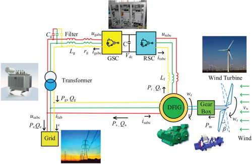
The configuration of a DFIG connected to a power grid is schematically illustrated in Figure 1. Here, an induction generator and a wind turbine are connected with a mechanical shaft system, which is directly connected to the power grid with its stator and a back-to-back converter with its rotor, respectively. The RSC controller aims to regulate the rotor speed and reactive power; while the grid side converter (GSC) controller attempts to maintain a constant DC link voltage from the variation of rotor power (Yang, Zhang, Yu, Shu, & Fang, 2017). Note that the modelling of GSC is ignored as this paper focuses on active power regulation. As a consequence, only the RSC controller design is considered.

Figure 1. The configuration of a grid-connected DFIG-based wind turbine (Yang et al., 2017).

2.1. Wind turbine model

The mechanical power captured by wind turbine can be written as (Fei & Pal, 2007; Yang, Jiang, Wang, Yao, & Wu, 2016): (1) $P_m=\frac{1}{2}\rho \pi R^2{C}_p\left(\lambda .\text{β}\right)v_{wind}^3,$(1) where r is the air density, $R$ denotes the radius of wind turbine and $v_{wind}$ means the wind speed. $C_P\left(\lambda .\text{β}\right)$ is a function of tip-speed-ratio $\lambda$ and blade pitch angle $\text{β}$ representing the power coefficient. A specific wind speed corresponds to a wind turbine rotational speed to obtain $C_{Pmax}$, namely, the maximum power coefficient, and therefore tracks the maximum mechanical (wind) power. In general, the wind turbine operates in the variable speed mode if wind speed does not exceed its rated value, then the rotational speed is adjusted by DFIG speed control so that $C_P\left(\lambda .\text{β}\right)$ can remain at the $C_{Pmax}$ point. However, if wind turbine operates above the rated wind speed, the pitch angle will be adjusted to guarantee the safe operation of the wind turbine. Finally, the tip-speed-ratio $\lambda$ can be defined as: (2) $\lambda =\frac{{\omega }_{m}R}{v_{wind}},$(2) where ${\omega }_m$ denotes the wind turbine rotational speed. According to the wind turbine characteristics, a generic equation of $C_P\left(\lambda .\text{β}\right)$ can be described by: (3) $C_p\left(\lambda .\text{β}\right)=c_1\left(\frac{c_2}{{\lambda }_i}-c_3\text{β}-c_4\right)e^{-\frac{c_5}{{\lambda }_i}}+c_6\lambda$(3) with (4) $\frac{1}{{\lambda }_i}=\frac{1}{\lambda +0.08\text{β}}-\frac{0.035}{{\text{β}}^3+1},$(4) where $c_1$ to $c_6$ are set to: $c_1=\mathrm{0.5176.}{c}_2=116.c_3=\mathrm{0.4.}{c}_4=5.c_5=21.c_6=0.0068$, respectively (Fei & Pal, 2007; Yang et al., 2016).

2.2. Generator model

The generator dynamics is given by: (5) $\begin{array}{rl}\frac{\text{d}{i}_{qs}}{\text{d}t}& =\frac{{\omega }_b}{{L^{\mathrm{\prime }}}_s}\left(-R_1{i}_{qs}+{\omega }_s{L^{\mathrm{\prime }}}_s{i}_{ds}+\frac{{\omega }_r}{{\omega }_s}{e^{\mathrm{\prime }}}_{qs}\right.\\ & -\left.\frac{1}{T_r{\omega }_s}{e^{\mathrm{\prime }}}_{ds}-v_{qs}+\frac{L_m}{L_{rr}}{v}_{qr}\right),\\ \frac{\text{d}{i}_{ds}}{\text{d}t}& =\frac{{\omega }_b}{{L^{\mathrm{\prime }}}_s}\left(-R_1{i}_{ds}-{\omega }_s{L^{\mathrm{\prime }}}_s{i}_{qs}+\frac{{\omega }_r}{{\omega }_s}{e^{\mathrm{\prime }}}_{ds}\right.\\ & +\left.\frac{1}{T_r{\omega }_s}{e^{\mathrm{\prime }}}_{qs}-v_{ds}+\frac{L_m}{L_{rr}}{v}_{dr}\right),\\ \frac{\text{d}{e^{\mathrm{\prime }}}_{qs}}{\text{d}t}& ={\omega }_b{\omega }_s\left(R_2{i}_{ds}+\left(1-\frac{{\omega }_r}{{\omega }_s}\right){e^{\mathrm{\prime }}}_{qs}\right.\\ & -\left.\frac{1}{T_r{\omega }_s}{e^{\mathrm{\prime }}}_{qs}-\frac{L_m}{L_{rr}}{v}_{dr}\right),\\ \frac{\text{d}{e^{\mathrm{\prime }}}_{ds}}{\text{d}t}& ={\omega }_b{\omega }_s\left(-R_2{i}_{qs}-\left(1-\frac{{\omega }_r}{{\omega }_s}\right){e^{\mathrm{\prime }}}_{qs}\right.\\ & -\left.\frac{1}{T_r{\omega }_s}{e^{\mathrm{\prime }}}_{ds}+\frac{L_m}{L_{rr}}{v}_{qr}\right),\end{array}$(5) where ${\omega }_b$ represents the electrical base speed, ${\omega }_s$ denotes the synchronous angle speed and ${\omega }_r$ means the rotor angle speed; $e_{ds}^{\mathrm{\prime }}$ and $e_{qs}^{\mathrm{\prime }}$ denote the equivalent d-axis and q-axis (dq) internal voltages; $i_{ds}$ and $i_{qs}$ are the dq-stator currents; $v_{ds}$ and $v_{qs}$ represent the dq-stator terminal voltages; $v_{dr}$ and $v_{qr}$ are the dq-rotor voltages. $L_m$ means the mutual inductance; while the remaining parameters are provided in the below. (6) $\begin{array}{rl}{\omega }_b& =100\pi \text{rad}/\text{s}.{\omega }_s=1p\cdot u,\\ L_m& =4p\cdot u.L_{ss}=1\cdot 01L_m.L_{rr}=1\cdot 005\\ L_{ss}.L_s\mathrm{\prime }& =L_{ss}-\frac{L_m^2}{L_{rr}}.H_m=4\cdot 4s,\\ R_s& =0\cdot 005p\cdot u.R_r=1\cdot 1R_s.R_2=(L_m/L_{rr}{)}^2{R}_r.\\ R_1& =R_s+R_2.T_r=L_{rr}/R_r,\\ \rho & =1\cdot 225\text{kg}/{\text{m}}^{\text{3}}.R=58\cdot 59{\text{m}}^{\text{2}}.\\ v_{wind}& =12\text{m}/\text{s}.\text{β}=15\text{deg}\text{.}\end{array}$(6) The active power $P_e$ produced by the generator is calculated by: (7) $P_e=e_{qs}^{\mathrm{\prime }}{i}_{qs}+e_{ds}^{\mathrm{\prime }}{i}_{ds}.$(7) The q-axis is aligned with the stator voltage while the d-axis is aligned to lead the q-axis, thus, $v_{ds}\equiv 0$ and $v_{qs}$ equals to the terminal voltage magnitude. The reactive power $Q_e$ is obtained as: (8) $Q_e=v_{qs}{i}_{ds}-v_{ds}{i}_{qs}.$(8)

2.3. Shaft system model

The shaft system can be modelled as a single lumped-mass system, whose lumped inertia constant $H_m$ is calculated as (Qiao, 2009): (9) $H_m=H_t+H_g,$(9) where $H_t$ and $H_g$ are the inertia constants of wind turbine and generator, respectively. The electromechanical dynamics is written as: (10) $\frac{\text{d}{\omega }_m}{\text{d}t}=\frac{1}{2H_m}\left(T_m-T_e-D{\omega }_m\right),$(10) where ${\omega }_m$ represents the rotational speed of the lumped-mass system equivalent to the generator rotor speed ${\omega }_r$; $D$ denotes the lumped system damping; and $T_m$ is the mechanical torque with $T_m=\left(P_m/{\omega }_m\right)$, respectively.

3. RAMPC design of DFIG for power system stability enhancement

Consider the following continuous time nonlinear system (11) $\dot{x}\left(t\right)=Ax\left(t\right)+Bu\left(t\right)+w\left(t.x\right),$(11) where $x\left(t\right)\in R^{n_x}$ shows the system states, $u\left(t\right)\in R^{n_u}$ the control input, $w\left(t.x\right):R^{n_x}\to R^{n_w}$ continuous nonlinear uncertainty function. The $w\left(t.x\right)$ is considered in the following set (12) $W=\left\{w\left(t.x\right)\in R^{n_w}|w\le w_{max}\right\}.$(12) The system has the following limitations $x\left(t\right)\in \overline{X}.u\left(t\right)\in \overline{U}.\mathrm{\forall }t>0$. Where $\overline{X}\subset R^{n_x}$ is bounded and $\overline{U}\subset R^{n_u}$ is compact.

Lemma 3.1

Yu, Böhm, Chen, & Allgöwer, 2010

Let $S:R^{n_x}\to \left[0.\mathrm{\infty }\right)$ be a continuously differentiable function and ${\alpha }_1\left(x\right)<S\left(x\right)<{\alpha }_2\left(x\right)$, where ${\alpha }_1,{\alpha }_2$ are $k_{\mathrm{\infty }}$ class functions. Suppose $u:R\to R^{n_u}$ is chosen, and there exit $\lambda >0$ and $\mu >0$ such that (13) $\dot{S}\left(x\right)+\lambda S\left(x\right)-\mu w^{\text{T}}\left(t.x\right)w\left(t.x\right)\le 0.$(13) With $x\in X.w\in W$. Then, the system trajectory starting from $x\left(t_0\right)\in \mathrm{\Omega }\subseteq X$ will remain in the set $\mathrm{\Omega }$, where (14) $\mathrm{\Omega }=\left\{x\in R^{n_x}|S\left(x\right)\le \frac{\mu w_{max}^2}{\lambda }\right\}.$(14)

Lemma 3.2

Poursafar, Taghirad, & Haeri, 2010

Let $M,N$ be real constant matrices and $P$ be a positive matrix of compatible dimensions. Then (15) $M^{T}PN+N^{T}PM\le \epsilon M^{T}PM+{\epsilon }^{-1}{N}^{T}PN.$(15) Holds for any $\epsilon >0$.

Lemma 3.3.

Schur complements Boyd, Ghaoui, Feron, & Balakrishnan, 1994

The LMI (16) $\left[\begin{array}{cc}Q\left(x\right)& S\left(x\right)\\ S^T\left(x\right)& R\left(x\right)\end{array}\right]>0.$(16) In which, $Q\left(x\right)=Q^T\left(x\right)$, $R\left(x\right)=R^T\left(x\right)$ and $S\left(x\right)$ are affine function of $x$, and is equivalent to (17) $\begin{array}{cc}R\left(x\right)>0& Q\left(x\right)-S\left(x\right)R^{-1}\left(x\right)S^T\left(x\right),\\ Q\left(x\right)>0& R\left(x\right)-S\left(x\right)Q^{-1}\left(x\right)S^T\left(x\right).\end{array}$(17) Choosing the tracking error $e={\left[\begin{array}{cc}{e}_1& e_2\end{array}\right]}^T$ of active power $P_e$ and reactive power $Q_e$ as the outputs, it yields (18) $\begin{array}{r}{e}_1=P_e-P_e^{\ast },\\ e_2=Q_e-Q_e^{\ast },\end{array}$(18) where $P_e^{\ast }$ and $Q_e^{\ast }$ denote the active power and reactive power references, respectively.

The derivative of tracking error (18) until control inputs $v_{qr}$ and $v_{dr}$ appeared explicitly, gives (19) $\begin{array}{rl}\left[\begin{array}{c}{\dot{e}}_1\\ {\dot{e}}_2\end{array}\right]& =\left[\begin{array}{cc}-\frac{R_1{\omega }_b}{L_s^{\mathrm{\prime }}}-\frac{{\omega }_b}{T_r}& 0\\ 0& -\frac{R_1{\omega }_b}{L_s^{\mathrm{\prime }}}\end{array}\right]\left[\begin{array}{c}{e}_1\\ e_2\end{array}\right]+\left[\begin{array}{c}{f}_1\\ f_1\end{array}\right]\\ & +\left[\begin{array}{cc}{B}_{11}& B_{12}\\ B_{21}& B_{22}\end{array}\right]\left[\begin{array}{c}{v}_{qr}\\ v_{dr}\end{array}\right],\end{array}$(19) where (20) $\begin{array}{rl}{f}_1& =-\frac{{\omega }_b}{{L^{\mathrm{\prime }}}_s}{v}_{qs}{e^{\mathrm{\prime }}}_{qs}-\frac{{\omega }_b}{L_s^{\mathrm{\prime }}}{v}_{ds}{e^{\mathrm{\prime }}}_{ds}+\frac{{\omega }_b{\omega }_r}{{L^{\mathrm{\prime }}}_s{\omega }_s}(e_{qs}^{\mathrm{\prime }2}+e_{ds}^{\mathrm{\prime }2})\\ & +{\omega }_b{\omega }_r\left({e^{\mathrm{\prime }}}_{qs}{i}_{ds}-{e^{\mathrm{\prime }}}_{ds}{i}_{qs}\right)-\left(\frac{R_1{\omega }_b}{{L^{\mathrm{\prime }}}_s}+\frac{{\omega }_b}{T_r}\right)P_e^{\ast }-{\dot{P}}_e^{\ast },\\ f_2& =-{\omega }_b{\omega }_s\left(v_{qs}{i}_{qs}+v_{ds}{i}_{ds}\right)+\frac{{\omega }_b}{{L^{\mathrm{\prime }}}_s{T}_r{\omega }_s}\left(v_{qs}{e^{\mathrm{\prime }}}_{qs}+v_{ds}{e^{\mathrm{\prime }}}_{ds}\right)\\ & +\frac{{\omega }_b{\omega }_r}{{L^{\mathrm{\prime }}}_s{\omega }_s}\left(v_{qs}{e^{\mathrm{\prime }}}_{ds}-v_{ds}{e^{\mathrm{\prime }}}_{qs}\right)-\frac{R_1{\omega }_b}{{L^{\mathrm{\prime }}}_s}{Q}_e^{\ast }-{\dot{Q}}_e^{\ast },\\ B_{11}& =\frac{L_m{\omega }_b}{L_{rr}{L^{\mathrm{\prime }}}_s}{e^{\mathrm{\prime }}}_{qs}+\frac{L_m{\omega }_b{\omega }_s}{L_{rr}}{i}_{ds},\\ B_{12}& =\frac{L_m{\omega }_b}{L_{rr}{L^{\mathrm{\prime }}}_s}{e^{\mathrm{\prime }}}_{qs}-\frac{L_m{\omega }_b{\omega }_s}{L_{rr}}{i}_{qs},\\ B_{21}& =-\frac{L_m{\omega }_b}{L_{rr}{L^{\mathrm{\prime }}}_s}{v}_{ds},\\ B_{22}& =\frac{L_m{\omega }_b}{L_{rr}{L^{\mathrm{\prime }}}_s}{v}_{qs},\end{array}$(20) where $f_1$ and $f_2$ include the combinatorial effect of nonlinearities, generator parameter uncertainties and external disturbances. Moreover, $B$ is the original control gain matrix which elements also contain uncertain generator parameters.

Assume all nonlinearities and parameters are unknown, define the perturbations ${\psi }_1(\cdot )$ and ${\psi }_2(\cdot )$ for system (19) to aggregate all the nonlinearities, generator uncertainties and external disturbances of $f_1,f_2$ and $B$ into a lumped term, such that they can be rewritten into a concise form, it yields (21) $\left[\begin{array}{c}{\psi }_1(\cdot )\\ {\psi }_2(\cdot )\end{array}\right]=\left[\begin{array}{c}{f}_1\\ f_1\end{array}\right]+\left(B-B_0\right)\left[\begin{array}{c}{v}_{qr}\\ v_{dr}\end{array}\right],$(21) where the new control gain $B_0$ is given by (22) $B_0=\left[\begin{array}{cc}{b}_{11}& 0\\ 0& b_{22}\end{array}\right],$(22) where $b_{11}$ and $b_{22}$ are constants. Here, the new control gain $B_0$ is chosen in such form to completely decouple the control of active power and reactive power.

Then system (19) can be rewritten as (23) $\begin{array}{rl}\left[\begin{array}{c}{\dot{e}}_1\\ {\dot{e}}_2\end{array}\right]& =\left[\begin{array}{cc}-\frac{R_1{\omega }_b}{L_s^{\mathrm{\prime }}-\frac{{\omega }_b}{T_r}}& 0\\ 0& -\frac{R_1{\omega }_b}{L_s^{\mathrm{\prime }}}\end{array}\right]\left[\begin{array}{c}{e}_1\\ e_2\end{array}\right]+\left[\begin{array}{c}{\psi }_1(\cdot )\\ {\psi }_2(\cdot )\end{array}\right]\\ & +\left[\begin{array}{cc}{b}_{11}& 0\\ 0& b_{22}\end{array}\right]\left[\begin{array}{c}{v}_{qr}\\ v_{dr}\end{array}\right].\end{array}$(23) Here, the above first order differential equations describe the decoupled dynamics of active power and reactive power, respectively.

By definition (24) $\begin{array}{r}{v}_{qr}=u_1+v_1,\\ v_{dr}=u_2+v_2.\end{array}$(24) where $v_1$ and $v_2$ are related to the adaptive state feedback, and $u_1$ and $u_2$ are related to the robust predictive control. State feedback provides the achievement of equilibrium and robust predictive control to ensure stability in the face of uncertainties.

The state-feedback section plays the role of achieving to the equilibrium point and the precursor precision control part plays the role of ensuring the consistency of the system against the uncertainties.

To get the adaptive state-feedback rule, we consider the Equation (25): (25) $\begin{array}{rl}\left[\begin{array}{c}{\dot{e}}_1\\ {\dot{e}}_2\end{array}\right]& =\left[\begin{array}{cc}-\frac{R_1{\omega }_b}{{L^{\mathrm{\prime }}}_s}-\frac{{\omega }_b}{T_r}& 0\\ 0& -\frac{R_1{\omega }_b}{{L^{\mathrm{\prime }}}_s}\end{array}\right]\left[\begin{array}{c}{e}_1\\ e_2\end{array}\right]+\left[\begin{array}{c}{\psi }_1(\cdot )\\ {\psi }_2(\cdot )\end{array}\right]\\ & +\left[\begin{array}{cc}{b}_{11}& 0\\ 0& b_{22}\end{array}\right]\left[\begin{array}{c}{v}_1\\ v_2\end{array}\right].\end{array}$(25) We select the Lyapunov function as follows. (26) $V\left(e_1,e_2\right)=\frac{1}{2}{e}_1^2+\frac{1}{2}{e}_2^2+\frac{1}{2{\alpha }_1}{\tilde{\psi }}_1^2(\cdot )+\frac{1}{2{\alpha }_2}{\tilde{\psi }}_2^2(\cdot ),$(26) where ${\alpha }_1,{\alpha }_2$ are adaptive law adjustment parameters, and also adaptive error will be as follows: (27) $\begin{array}{cc}{\tilde{\psi }}_1(\cdot )={\psi }_1(\cdot )-{\hat{\psi }}_1(\cdot )& {\tilde{\psi }}_2(\cdot )={\psi }_2(\cdot )-{\hat{\psi }}_2(\cdot )\end{array}.$(27)

By selecting adaptive state feedback as follows: (28) $\begin{array}{r}{v}_1=-k_1{e}_1-\frac{{\hat{\psi }}_1(\cdot )}{b_{11}},\\ v_2=-k_2{e}_2-\frac{{\hat{\psi }}_2(\cdot )}{b_{22}}.\end{array}$(28) In order to guarantee the stability, the derivative of the Lyapunov function must be negative. For this purpose (29) $\begin{array}{rl}\dot{V}\left(e_1,e_2\right)& =e_1\left(-\left(\frac{R_1{\omega }_b}{{L^{\mathrm{\prime }}}_s}+\frac{{\omega }_b}{T_r}\right)e_1-b_{11}{k}_1{e}_1\right)\\ & +e_2\left(-\frac{R_1{\omega }_b}{{L^{\mathrm{\prime }}}_s}{e}_2-b_{22}{k}_2{e}_2\right)\\ & +{\tilde{\psi }}_1(\cdot )\left(e_1-\frac{1}{{\alpha }_1}{\hat{\psi }}_1(\cdot )\right)\\ & +{\tilde{\psi }}_2(\cdot )\left(e_2-\frac{1}{{\alpha }_2}{\hat{\psi }}_2(\cdot )\right).\end{array}$(29) By choosing the adaptive law as follows (30) $\begin{array}{r}{\hat{\psi }}_1(\cdot )={\alpha }_1{e}_1,\\ {\hat{\psi }}_2(\cdot )={\alpha }_2{e}_2.\end{array}$(30) We will have (31) $\begin{array}{rl}\dot{V}\left(e_1,e_2\right)& =-\left(\frac{R_1{\omega }_b}{{L^{\mathrm{\prime }}}_s}+\frac{{\omega }_b}{T_r}+b_{11}{k}_1\right)e_1^2\\ & -\left(\frac{R_1{\omega }_b}{{L^{\mathrm{\prime }}}_s}+b_{22}{k}_2\right)e_2^2.\end{array}$(31)

Applying (29) and (31) to (23) and rewriting it, we have (32) $\begin{array}{rl}\left[\begin{array}{c}{\dot{e}}_1\\ {\dot{e}}_2\end{array}\right]& =\left[\begin{array}{c}-\left(\frac{R_1{\omega }_b}{{L^{\mathrm{\prime }}}_s}+\frac{{\omega }_b}{T_r}+b_{11}{k}_1-\frac{{\hat{\psi }}_1(\cdot )}{b_{11}}\right)\\ 0\end{array}\right.\\ & \left.\begin{array}{c}0\\ -\left(\frac{R_1{\omega }_b}{{L^{\mathrm{\prime }}}_s}+b_{22}{k}_2-\frac{{\hat{\psi }}_2(\cdot )}{b_{22}}\right)\end{array}\right]\left[\begin{array}{c}{e}_1\\ e_2\end{array}\right]+\left[\begin{array}{c}{\psi }_1(\cdot )\\ {\psi }_2(\cdot )\end{array}\right]\\ & +\left[\begin{array}{cc}{b}_{11}& 0\\ 0& b_{22}\end{array}\right]\left[\begin{array}{c}{u}_1\\ u_2\end{array}\right].\end{array}$(32) Now, with the intention to control the system (32), we will apply robust predictive control.

The state-feedback control law for system (32) in $kT$ time is chosen as (33) $u\left(kT+\tau ,kT\right)=Ke\left(kT+\tau ,kT\right).$(33)

The chosen infinite horizon quadratic cost function is specified as (34) $\begin{array}{rl}J& ={\int }_0^{\mathrm{\infty }}\left(e{\left(kT+\tau ,kT\right)}^{T}Qe\right(kT+\tau ,kT)\\ & +u{\left(kT+\tau ,kT\right)}^{T}Ru\left(kT+\tau ,kT\right)-\mu w{\left(kT+\tau ,kT\right)}^T\\ & \times w\left(kT+\tau ,kT\right))d\tau ,\mu >0,\end{array}$(34) where $Q$ and $R$ are positive definite weight matrices. In the objective function (34), the uncertainties negative effect with weight $\mu$ is introduced, where $\mu$ is obtained by $H_{\mathrm{\infty }}$ method (Tahir & Jaimoukha, 2011).

Theorem 3.1:

Consider system (32), $e\left(kT\right)$ is the measured value in sampling time of $kT$. There is a state-feedback control law (33) that is true in stability condition. If the optimization problem with LMI constraints can be feasible. (35) $\begin{array}{c}\begin{array}{c}\text{min}\gamma \\ \gamma .X\end{array}\\ \begin{array}{c}\left[\begin{array}{cc}I& e{\left(kT\right)}^T\\ e\left(kT\right)& X\end{array}\right]\ge 0\\ {\left(AX+BY\right)}^T+AX+BY+\left(\alpha +\lambda \right)X\le 0\\ -X+\gamma {\epsilon }^{-1}I\le 0,\end{array}\end{array}$(35) where $X>0$, $Y$ are matrixes obtained from the above-mentioned optimization problem. As such, the state-feedback matrix in every moment is obtained as $K=Y{X}^{-1}$.

Proof:

Considering a quadratic Lyapunov function, we have (36) $V\left(e\left(t\right)\right)=e(t{)}^{T}Pe\left(t\right),P>0.$(36) In sampling time, assume that $V\left(e\left(t\right)\right)$ satisfies the following condition (37) $e(t{)}^{T}Pe\left(t\right)<\gamma ,$(37) (38) $\begin{array}{rl}\frac{dV\left(e\left(kT+\tau .kT\right)\right)}{dt}& \le -\left(e{\left(kT+\tau ,kT\right)}^{T}Qe\right(kT+\tau ,kT)\\ & +u{\left(kT+\tau ,kT\right)}^{T}Ru\left(kT+\tau ,kT\right)\\ & -\mu w{\left(kT+\tau ,kT\right)}^{T}w\left(kT+\tau ,kT\right)).\end{array}$(38) In order to obtain the robust efficiency, we should have $e\left(\mathrm{\infty },kT\right)=0$ which results in $V\left(e\left(\mathrm{\infty },kT\right)\right)=0$. By integrating both sides of the Equation (38), we have (39) $J\le V\left(e\left(kT\right)\right),$(39) where $\gamma$ is a positive scalar (the upper bound of the objective (34)).

In order to obtain an MPC robust algorithm, the Lyapunov function should be minimized considering the upper bound (Ghaffari, Vahid Naghavi, Safavi, & Shafiee, 2013). So (40) $\begin{array}{c}\text{min}\gamma \\ \gamma .P\\ \begin{array}{c}\text{subject to}\\ e{\left(t\right)}^{T}Pe\left(t\right)\le \gamma .\end{array}\end{array}$(40) By defining $X=\gamma P^{-1}$ and using Schur Complements, we have (41) $\begin{array}{c}\text{min}\gamma \\ \gamma .X\\ \left[\begin{array}{cc}I& x{\left(kT\right)}^T\\ x\left(kT\right)& X\end{array}\right]\ge 0\end{array}$(41)

According to Lemma 1, for system (32) we have (42) $\dot{S}\left(e\left(t\right)\right)+\lambda S\left(e\left(t\right)\right)-\mu w(t,e{)}^{T}w\left(t,e\right)\le 0.$(42) Then, according to (36) we have (43) $\begin{array}{rl}& \dot{e}(t{)}^{T}Pe\left(t\right)+e(t{)}^{T}P\dot{e}\left(t\right)+\lambda e(t{)}^{T}Pe\left(t\right)\\ & -\mu w(t,e{)}^{T}w\left(t,e\right)\le 0,\end{array}$(43) (44) $\begin{array}{rl}& e(t{)}^T\left({\left(A+BK\right)}^{T}P+P\left(A+BK\right)+\lambda P\right)e\left(t\right)\\ & +w(t,e{)}^{T}Pe\left(t\right)+e(t{)}^{T}Pw\left(t,e\right)-\mu w(t,e{)}^{T}w\left(t,e\right)\le 0.\end{array}$(44) According to Lemma 2, we have (45) $\begin{array}{rl}& w(t,e{)}^{T}Pe\left(t\right)+e(t{)}^{T}Pw\left(t,e\right)\le \alpha e(t{)}^{T}Pe\left(t\right)\\ & +{\alpha }^{-1}w(t,e{)}^{T}Pw\left(t,e\right).\end{array}$(45) By substituting (45) in (44), it is obtained that (46) $\begin{array}{rl}& e(t{)}^T\left({\left(A+BK\right)}^{T}P+P\left(A+BK\right)+\left(\alpha +\lambda \right)P\right)e\left(t\right)\\ & +{\alpha }^{-1}w(t,e{)}^{T}Pw\left(t,e\right)-\mu w(t,e{)}^{T}w\left(t,e\right)\le 0.\end{array}$(46) Consider (47) $P\le {\lambda }_{max}I\le \epsilon I,$(47) where ${\lambda }_{max}$ is the maximum eigenvalue of $P$ and $\epsilon I$ is the corresponding upper bound (Poursafar et al., 2010), then (48) $\begin{array}{rl}& e(t{)}^T\left({\left(A+BK\right)}^{T}P+P\left(A+BK\right)+\left(\alpha +\lambda \right)P\right)e\left(t\right)\\ & +\left({\alpha }^{-1}\epsilon -\mu \right)w(t.e{)}^{T}w\left(t.e\right)\le 0.\end{array}$(48) By choosing (49) $\mu =\frac{\epsilon }{\alpha }.$(49) Equation (48) is reduced to (50) $e(t{)}^T\left({\left(A+BK\right)}^{T}P+P\left(A+BK\right)+\left(\alpha +\lambda \right)P\right)e\left(t\right)\le 0.$(50)

By substituting $P=\gamma X^{-1}.X>0$ and $K=Y{X}^{-1}$, (51) $\begin{array}{rl}& ({\left(A+BY{X}^{-1}\right)}^T{X}^{-1}+X^{-1}(A+BY{X}^{-1})\\ & +\left(\alpha +\lambda \right)X^{-1})\gamma \le 0.\end{array}$(51) Pre and post multiplying by $X$, (52) $(AX+BY{)}^T+AX+BY+\left(\alpha +\lambda \right)X\le 0.$(52) Given (47), we have (53) $P\le \epsilon I.$(53) Substituting $P=\gamma X^{-1}$ and pre multiplying by $X$, we have (54) $-X+\gamma {\epsilon }^{-1}I\le 0.$(54) So, the proof is completed.

4. Simulation

In this section, the robust predictive control is applied to the DFIG system. Also, to prove the superiority of the proposed controller, it is compared with RPC (Dong et al., 2017). For this purpose, the controller parameters are selected as follows.

4.1. Step change of wind speed

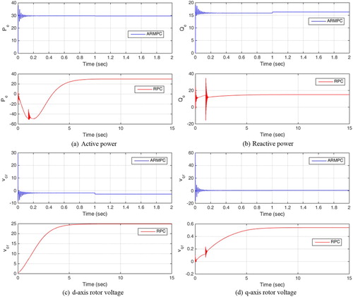
A step change of wind speed from 10 to 12 m/s (10 m/s² rate) with a fixed pitch angle of 15 degrees is tested, the wind speed profile and system responses and control costs are provided in Figure 2. It can be found that RPC control presents a 5 s active power oscillation while RAMPC can effectively suppress such unfavourable oscillation in less than 0.5 s, together with the minimal overshoot among all approaches. In addition, RAMPC needs the least control cost compared to that of RPC control. Although RAMPC restores the reactive power slower than the RPC control, it presents a smoother response with less overshoot.

Figure 2. System responses and control costs obtained under a step change of wind speed from 10 to 12 m/s with a fixed pitch angle of 15 deg. (a) active power; (b) reactive power; (c) d-axis rotor voltage; (d) q-axis rotor voltage.

4.2. Pitch angle variation

A pitch angle reduction that starts from 15 to 5 deg. in 1 s with a constant wind speed of 12 m/s is applied to compare the control performance of RAMPC against to that of RPC, while pitch angle is very crucial for the wind power production and secure operation of wind turbine (Duong, Grimaccia, Leva, Mussetta, & Ogliari, 2014). The system responses are given in Figure 3, which show that the active power of RAMPC can converge around 0.5 s, while RPC control needs to consume 10 s. In addition, RAMPC needs the least control costs compared to that of RPC control.

Figure 3. System responses obtained under a pitch angle variation from 15 to 5 deg. in 1 s with a constant wind speed of 12 m/s. (a) active power; (b) reactive power; (c) d-axis rotor voltage; (d) q-axis rotor voltage.

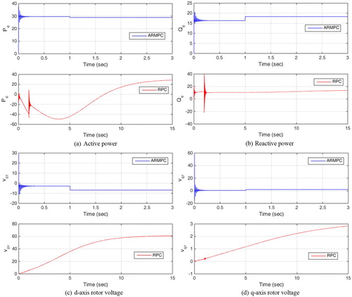
The comparisons show that the RAMPC strategy based on the nonlinear DFIG model can effectively track the given power set points in the presence of wind speed and pitch angle variations regardless of optimizing the cost function and considering constraints.

5. Conclusion

An LMI-based RAMPC strategy for DFIG-based WECS has been proposed in this paper. A DFIG model was considered and the predicted active and reactive output power were calculated using a state space model resulting in the nonlinear DFIG model. The control law is derived from LMI-based RAMPC that considers adaptive control law as an internal feedback loop for uncertainty, disturbance and nonlinear effects compensation and RMPC as an external feedback loop for overall system stability assurance. Also, it considers tracking problem and economic index through optimization of an objective function, while holds the constraints on the states and the control signal. It is shown that the performance of the proposed RAMPC is superior to the RPC method. Therefore, the proposed RAMPC provides a useful method for controlling this class of nonlinear DFIG in the operation of WECS in presence of wind variation and parameter uncertainty.

Disclosure statement

No potential conflict of interest was reported by the authors.

References

- Boyd, S., Ghaoui, L., Feron, E., & Balakrishnan, V. (1994). Linear matrix inequalities in control theory. SIAM, Philadelphia.
- Chisci, L., Rossiter, J., & Zappa, G. (2001). Systems with persistent disturbances: Predictive control with restricted constraints. Automatica, 37, 1019–1028. doi: 10.1016/S0005-1098(01)00051-6
- Chondrogiannis, S., & Barnes, M. (2008). Stability of doubly-fed induction generator under stator voltage orientated vector control. IET Renewable Power Generation, 2, 170–180. doi: 10.1049/iet-rpg:20070086
- Depenbrock, M. (1988). Direct self-control (DSC) of inverter-fed induction machine. IEEE Transactions on Power Electronics, 3, 420–429. doi: 10.1109/63.17963
- Dong, J., Li, S., Wu, S., He, T., Yang, B., Shu, H., & Yu, J. (2017). Nonlinear observer-based robust passive control of doubly-fed induction generators for power system stability enhancement via energy reshaping. Energies, 10, 1082. doi: 10.3390/en10081082
- Duong, M., Grimaccia, F., Leva, S., Mussetta, M., & Ogliari, E. (2014). Pitch angle control using hybrid controller for all operating regions of SCIG wind turbine system. Renewable Energy, 70, 197–203. doi: 10.1016/j.renene.2014.03.072
- Fei, M., & Pal, B. (2007). Modal analysis of grid-connected doubly fed induction generators. IEEE Transactions on Energy Conversion, 22, 728–736. doi: 10.1109/TEC.2006.881080
- Ghaffari, V., Vahid Naghavi, S., Safavi, A. A., & Shafiee, M. (2013). An LMI framework to design robust MPC for a class of nonlinear uncertain systems. Control Conference (ASCC), Asian.
- Grimm, G., Messina, M., Tuna, S., & Teel, A. (2003). Nominally robust model predictive control with state constraints. 42nd IEEE Conference on decision and control, Maui, Hawaii.
- Hao, S., Abdi, E., Barati, F., & McMahon, R. (2009). Stator-flux-oriented vector control for brushless doubly fed induction generator. IEEE Transactions on Industrial Electronics, 56, 4220–4228. doi: 10.1109/TIE.2009.2024660
- Hopfensperger, B., Atkinson, D., & Lakin, R. (2000). Stator-flux-oriented control of a doubly-fed induction machine with and without position encoder. IEE Proceedings – Electric Power Applications, 147, 241–250. doi: 10.1049/ip-epa:20000442
- Hu, J., He, Y., Xu, L., & Williams, B. (2009). Improved control of DFIG systems during network unbalance using PI–R current regulators. IEEE Transactions on Industrial Electronics, 56, 439–451. doi: 10.1109/TIE.2008.2006952
- Hu, J., Zhu, J., & Dorrell, D. (2014). Model-predictive direct power control of doubly-fed induction generators under unbalanced grid voltage conditions in wind energy applications. IET Renewable Power Generation, 8, 687–695. doi: 10.1049/iet-rpg.2013.0312
- Imani, H., Fazeli, S., Malekizade, H., & Hosseinzadeh, H. (2019). Tube model predictive control for a class of nonlinear discrete-time systems. Cogent Engineering, 1629055.
- Imani, H., Jahed-Motlagh, M., Salahshoor, K., Ramezani, A., & Moarefianpur, A. (2017). A novel tube model predictive control for surge instability in compressor system including piping acoustic. Cogent Engineering, 4(1), 1409373. doi: 10.1080/23311916.2017.1409373
- Imani, H., Jahed-Motlagh, M., Salahshoor, K., Ramezani, A., & Moarefianpur, A. (2018). Robust decentralized model predictive control approach for a multi-compressor system surge instability including piping acoustic. Cogent Engineering, 5(1), 1483811. doi: 10.1080/23311916.2018.1483811
- Imani, H., Malekizade, H., Asadi Bagal, H., & Hosseinzadeh, H. (2018). Surge explicit nonlinear model predictive control using extended Greitzer model for a CCV supported compressor. Automatika, 59(1), 43–50. doi: 10.1080/00051144.2018.1498204
- Landau, Ioan Doré, Lozano, Rogelio, M'Saad, Mohammed, & Karimi, Alireza. (2011). Adaptive Control Algorithms, Analysis and Applications. London: Springer-Verlag ISBN 978-0-85729-664-1. doi: 10.1007/978-0-85729-664-1
- Limon, D., Alamo, T., & Camacho, E. (2002). Input-to-state stable MPC for constrained discrete-time nonlinear systems with bounded additive uncertainties. 41th IEEE Conference on Decision and control, Las Vegas, NV, USA.
- Limon, D., Alamo, T., & Camacho, E. (2002). Stability analysis of systems with bounded additive uncertainties based on invariant sets: Stability and feasibility of MPC. American control Conference, Anchorage.
- Liserre, M., Cardenas, R., Molinas, M., & Rodriguez, J. (2011). Overview of multi-MW wind turbines and wind parks. IEEE Transactions on Industrial Electronics, 58(4), 1081–1095. doi: 10.1109/TIE.2010.2103910
- Magni, L., De Nicolao, G., & Scattolini, R. (1998). Output feedback recedinghorizon control of discrete-time nonlinear systems. 4th IFAC NOLCOS, Oxford, UK.
- Pena, R., Clare, J., & Asher, G. (1996). Doubly fed induction generator using back-to-back PWM converters and its application to variable-speed wind-energy generation. IEE Proceedings – Electric Power Applications, 143, 231–241. doi: 10.1049/ip-epa:19960288
- Poursafar, N., Taghirad, H., & Haeri, M. (2010). Model predictive control of nonlinear discrete time systems: A linear matrix inequality approach. IET Control Theory & Applications, 4, 1922–1932. doi: 10.1049/iet-cta.2009.0650
- Qiao, W. (2009). Dynamic modeling and control of doubly fed induction generators driven by wind turbines. Proceedings of the IEEE/PES power systems Conference and Exposition, Seattle, WA, USA.
- Richards, A., & How, J. (2006). Robust stable model predictive control with constraint tightening. Proceedings of the American control Conference, Minneapolis, MN.
- Sathiyanarayanan, J., & Senthil Kumar, A. (2014). Doubly fed induction generator wind turbines with fuzzy controller: A survey. The Scientific World Journal, 2014, 1–8. doi: 10.1155/2014/252645
- Scokaert, P., Rawlings, J., & Meadows, E. (1997). Discrete-time stability with perturbations: Application to model predictive control. Automatica, 33(3), 463–470. doi: 10.1016/S0005-1098(96)00213-0
- Sun, X., Zhang, B., Tang, X., McLellan, B., & Höök, M. (2016). Sustainable energy transitions in China: Renewable options and impacts on the electricity system. Energies, 9, 980. doi: 10.3390/en9120980
- Tahir, F., & Jaimoukha, I. M. (2011). Robust model predictive control through dynamic state-feedback: An LMI approach. Preprints of the 18th IFAC World Congress, Milano, Italy.
- Takahashi, I., & Noguchi, T. (1986). A new quick-response and high-efficiency control strategy of an induction motor. IEEE Transactions on Industry Applications, IA-22, 820–827. doi: 10.1109/TIA.1986.4504799
- Taleb Ziabari, M., Jahed-Motlagh, M. R., Salahshoor, K., Ramezani, A., & Moarefianpur, A. (2017). Robust adaptive control of surge instability in constant speed centrifugal compressors using tube-MPC. Cogent Engineering, 4(1), 1339335. doi: 10.1080/23311916.2017.1339335
- Yang, B., Jiang, L., Wang, L., Yao, W., & Wu, Q. (2016). Nonlinear maximum power point tracking control and modal analysis of DFIG based wind turbine. International Journal of Electrical Power & Energy Systems, 74, 429–436. doi: 10.1016/j.ijepes.2015.07.036
- Yang, B., Zhang, X., Yu, T., Shu, H., & Fang, Z. (2017). Grouped grey wolf optimizer for maximum power point tracking of doubly-fed induction generator based wind turbine. Energy Conversion and Management, 133, 427–443. doi: 10.1016/j.enconman.2016.10.062
- Yu, S.-Y., Böhm, C., Chen, H., & Allgöwer, F. (2010). Robust model predictive control with disturbance invariant sets. Proceedings of the American control Conference, Baltimore, MD.
- Zhi, D., & Xu, L. (2007). Direct power control of DFIG with constant switching frequency and improved transient performance. IEEE Transactions on Energy Conversion, 22, 110–118. doi: 10.1109/TEC.2006.889549
- Zhi, D., Xu, L., & Williams, B. (2010). Model-based predictive direct power control of doubly fed induction generators. IEEE Transactions on Power Electronics, 25, 341–351.