Stabilization of piecewise-homogeneous Markovian switching CVNNs with mode-dependent delays and incomplete transition rates

Abstract

This paper is devoted to the problems of exponential stability and stabilization for piecewise-homogeneous Markovian switching complex-valued neural networks with incomplete transition rates (TRs). Both the time-varying delays and the coefficient matrices are switched among finite modes governed by a piecewise-homogeneous Markov process, where the TRs of the two-level Markov processes are assumed to be time-varying during different intervals. On the basis of an appropriately chosen Lyapunov–Krasovskii functional, some mode-dependent sufficient conditions are presented to guarantee the unforced network to be exponentially mean-square stable. Then, by proposing certain mode-dependent state feedback controller, stabilization criteria are derived through strict mathematical proofs. At the end of the paper, numerical examples are provided to illustrate the effectiveness of the theoretical results.

Keywords:

• Complex-valued neural networks
• piecewise-homogeneous Markovian switching
• stabilization
• incomplete transition rates

1. Introduction

In the past decades, much attention has been gathered to complex-valued neural networks (CVNNs) due to their extensive practical applications in pattern recognition, signal processing, associative memories, target tracking and combinatorial optimization (Goh & Mandic, 2004, 2007; Hirose, 1992a, 1992b; Jankowski et al., 1996). CVNNs can be regarded as an extension of the real-valued neural networks, where the system states, external inputs, connection weights, and activation functions are all complex-valued. From this point of view, it can be utilized to deal with the high-dimensional data or the complex states composed of amplitude and phase. Therefore, there has been an enormous interest in the research of CVNNs, and a great many of interesting results have been proposed, see Refs. Song and Zhao (2016), Kobayashi (2018), Gong et al. (2015), Wang et al. (2016), Liu and Chen (2015), Liang et al. (2016), Li et al. (2019) and the references cited therein, for example.

On another front, time delays are inevitably pervasive in the processing of information due to the finite transmission speed of signals travelling through the links (Anderson & Spong, 1989; Luo et al., 2017; Wang et al., 2018). It is worth noting that the existence of the time delays may lead to oscillation or even instability of the systems under consideration. Up to now, many kinds of delays have been proposed for numerous practical systems, such as probabilistic time-varying delay, leakage delay, asynchronous time delay, distributed delay, proportional delay, and so on. At the same time, a great many significant dynamic results have been reported. For example, finite-time synchronization control problem has been tackled in C. Zhang, et al. (2018) for a class of fully CVNNs with coupling delay. The attracting and invariant sets have been investigated in Yang and Liao (2019) for the non-autonomous CVNNs with time-varying delays and infinite distributed delay. Leakage delay-dependent asymptotic stability has been considered in Samidurai et al. (2019) for a class of CVNNs with discrete/distributed time-varying delays. When referring to the stability/stabilization issue on CVNNs with mode-dependent time-varying delays, there has been little research attention on that. Such a situation motivates our present research.

It should be noted that, so far, Markovian switching systems (MSSs) have witnessed a significant progress due to the fact that MSS can describe the random abrupt changes and the environmental variance, which might be governed by a Markovian process or Markovian chain with finite modes (Liu et al., 2018; Luo et al., 2020; Ma et al., 2018; Zhang et al., 2019). During the past years, a great many of relevant results for Markovian switching neural networks (MSNNs) with time delays have been introduced (Nagamani et al., 2017; Zhang et al., 2015; T. Zhang, et al., 2018). For instance, the dissipativity and passivity problem has been investigated in Nagamani et al. (2017) for the impulsive neural networks with both Markovian jumping parameters and mixed time delays. Asymptotic synchronization of coupled reaction–diffusion neural networks with proportional delay and Markovian switching topologies has been addressed in Yang et al. (2018). Furthermore, the stability analysis problem of CVNNs with Markovian topology is also proposed in Wang et al. (2019), and the references cited therein.

It is noteworthy that in all the above-mentioned references, the transition rates (TRs) of the Markovian process are time-invariant and completely known, i.e. the considered Markovian process is assumed to be homogeneous. However, in fact, exact information of the TRs is mostly difficult to be measured and acquired because of the existence of random factors. Hence, it is important and urgent to study the MSSs with partly known TRs. Recently, some effects have been devoted to address the control synthesis problem for those kinds of systems (Du et al., 2013; Guo, 2016; Song et al., 2014; Zhang & Boukas, 2009). In addition to this, an interesting extension is to further consider the case that the TRs of the Markovian process are assumed to be time-varying, i.e. the Markovian process is nonhomogeneous. To be more specific, in Zhang (2009), the so-called piecewise-homogeneous Markovian process is firstly introduced, where the Markovian process contains finite consecutive homogeneous Markovian sub-chains with different intervals, longer or shorter. The TRs of the piecewise-homogeneous process are time-varying in different intervals but invariant during one interval, which can be viewed to mediate the homogeneous and nonhomogeneous ones. Corresponding results concerning systems with these kinds of time-varying TRs have been reported in Refs. Wu et al. (2012a) and Shen et al. (2016). To the best of the authors' knowledge, when taking the piecewise-homogeneous Markovian switching with partly known TRs into account, few results associated with the stability/stabilization problems can be found in the literature for CVNNs with mode-dependent time-varying delays, which forms one of the main motivations to promote the present research.

This paper aims to investigate the stability and stabilization problem for piecewise-homogeneous Markovian switching CVNNs with mode-dependent time-varying delays and incomplete TRs. More specially, by constructing an appropriate Lyapunov–Krasovskii functional candidate, combining with the generalized free-weighting-matrix technique, stability/stabilization criteria are to be established for the considered neural network. The main novelties of the present work are highlighted from the following four aspects.

• This is the first few attempts to tackle the stability/stabilization problem for piecewise-homogeneous Markovian switching CVNNs, where all the parameter matrices are switching according to a piecewise-homogeneous Markovian process.

• The TRs information of the TR matrix Π for the piecewise-homogeneous Markovian process is partly known, which has been seldom considered.

• To further generalize the system concerned time-varying delays are also assumed to be dependent on the piecewise-homogeneous Markovian process.

• Based on the Lyapunov stability theory, stochastic analysis technique and the generalized free-weighting-matrix method, sufficient mode/delay-dependent stability/stabilization conditions are derived for the complex-valued network under consideration.

The remainder of this paper is organized as follows. In Section 2, the piecewise-homogeneous Markovian switching CVNN model is proposed, and some necessary preliminaries are briefly shown. In Section 3, we establish some criteria for the stability and stabilization of the addressed systems by using the generalized free-weighting-matrix inequality method. Some numerical simulations are presented to show effectiveness of the obtained results in Section 4. Finally, conclusion of this paper is drawn in Section 5.

Notation

The notation used throughout this paper is fairly standard. ${\mathbb{C}}^n$, ${\mathbb{R}}^n$, ${\mathbb{C}}^{m\times n}$ and ${\mathbb{R}}^{m\times n}$ denote, respectively, the set of n-dimensional complex vectors, n-dimensional real vectors, $m\times n$ complex and real matrices. I is the identity matrix of appropriate dimensions. The superscript ‘T ’ denotes matrix transposition, and ‘⊗’ stands for the Kronecker product. Let $(\mathrm{\Omega },\mathcal{F},\{{\mathcal{F}}_t{\}}_{t\ge 0},\mathcal{P})$ be a complete probability space with a filtration $\{{\mathcal{F}}_t{\}}_{t\ge 0}$ satisfying the usual condition (i.e. the filtration ${\mathcal{F}}_0$ contains all $\mathcal{P}$-null sets and ${\mathcal{F}}_t$ is monotonically right continuous). The imaginary unit is denoted as $\overrightarrow{\mathrm{i}}$, i.e. $\overrightarrow{\mathrm{i}}\triangleq \sqrt{-1}$. ${\lambda }_{\mathrm{m}\mathrm{a}\mathrm{x}}\left(A\right)$ and ${\lambda }_{\mathrm{m}\mathrm{i}\mathrm{n}}\left(A\right)$ are the largest and smallest eigenvalues of matrix A. In a symmetric matrix, ‘$\ast$’ denotes the entries induced by symmetry. $\mathrm{c}\mathrm{o}\mathrm{l}(A_{\upsilon }{)}_{\upsilon =1}^n$ and $\mathrm{d}\mathrm{i}\mathrm{a}\mathrm{g}\{A_{\upsilon }{\}}_{\upsilon =1}^n$ refer to $(A_1^{\mathrm{T}},A_2^{\mathrm{T}},\dots ,A_n^{\mathrm{T}}{)}^{\mathrm{T}}$ and $\mathrm{d}\mathrm{i}\mathrm{a}\mathrm{g}\{A_1,A_2,\dots ,A_n\}$, respectively. $\mathbb{E}\{\cdot \}$ stands for the mathematical expectation of ‘·’.

2. Model formulation and preliminaries

Consider the following Markovian CVNNs with mode-dependent time-varying delay: (1) $\begin{array}{rl}\dot{z}\left(t\right)& =-C\left(r\right(t\left)\right)z\left(t\right)+A\left(r\right(t\left)\right)f\left(z\right(t\left)\right)\\ & +B\left(r\right(t\left)\right)g\left(z\right(t-{\tau }_{r\left(t\right),\sigma \left(t\right)}\left(t\right)\left)\right)+\tilde{u}\left(t\right),t\ge 0\end{array}$(1) where $z\left(t\right)=\mathrm{c}\mathrm{o}\mathrm{l}\left(z_{\upsilon }\right(t){)}_{\upsilon =1}^n\in {\mathbb{C}}^n$ is the state vector of the neural network with n neurons at time t, $C\left(r\right(t\left)\right)=\mathrm{d}\mathrm{i}\mathrm{a}\mathrm{g}\left\{c_{\upsilon }\right(r\left(t\right)){\}}_{\upsilon =1}^n\in {\mathbb{R}}^{n\times n}$ is the self-feedback connection weight matrix with positive entries $c_{\upsilon }\left(r\right(t\left)\right)>0$, $A\left(r\right(t\left)\right)=\left(a_{\upsilon \kappa }\right(r\left(t\right)){)}_{n\times n}\in {\mathbb{C}}^{n\times n}$ and $B\left(r\right(t\left)\right)=\left(b_{\upsilon \kappa }\right(r\left(t\right)){)}_{n\times n}\in {\mathbb{C}}^{n\times n}$ are, respectively, the connection weight matrix and the delayed connection weight matrix. $\tilde{u}\left(t\right)\in {\mathbb{C}}^n$ denotes the external control input vector. $f\left(z\right(t\left)\right)=\mathrm{c}\mathrm{o}\mathrm{l}\left(f_{\upsilon }\right(z_{\upsilon }\left(t\right)){)}_{\upsilon =1}^n:{\mathbb{C}}^n\to {\mathbb{C}}^n$ and $g\left(z\right(t\left)\right)=\mathrm{c}\mathrm{o}\mathrm{l}\left(g_{\upsilon }\right(z_{\upsilon }\left(t\right)){)}_{\upsilon =1}^n:{\mathbb{C}}^n\to {\mathbb{C}}^n$ are vector-valued nonlinear functions. ${\tau }_{r\left(t\right),\sigma \left(t\right)}\left(t\right)$ represents the mode-dependent time-varying delay satisfying $0<{\tau }_1\le {\tau }_{r\left(t\right),\sigma \left(t\right)}\left(t\right)\le {\tau }_2$ and ${\dot{\tau }}_{r\left(t\right),\sigma \left(t\right)}\left(t\right)\le \overline{\tau }$. The stochastic process $\left\{r\right(t),t\ge 0\}$ is a continuous-time non-homogeneous Markov process, which takes values in a finite set $\mathcal{S}\triangleq \{1,2,\dots ,N\}$ with TR matrix ${\mathrm{\Lambda }}^{\sigma (t+\mathrm{\Delta }t)}\triangleq [{\lambda }_{ij}^{\sigma (t+\mathrm{\Delta }t)}{]}_{N\times N}$ defined as follows: (2) $\begin{array}{rl}& \mathcal{P}\left\{r\right(t+\mathrm{\Delta }t)=j|r(t)=i\}\\ & =\left\{\begin{array}{ll}{\lambda }_{ij}^{\sigma (t+\mathrm{\Delta }t)}\mathrm{\Delta }t+o\left(\mathrm{\Delta }t\right),& i\ne j\\ 1+{\lambda }_{ii}^{\sigma (t+\mathrm{\Delta }t)}\mathrm{\Delta }t+o\left(\mathrm{\Delta }t\right),& i=j\end{array}\right.\end{array}$(2) in which $\mathrm{\Delta }t>0$, $\underset{\mathrm{\Delta }t\to 0}{lim}\left(o\right(\mathrm{\Delta }t\left)/\mathrm{\Delta }t\right)=0$, and ${\lambda }_{ij}^{\sigma (t+\mathrm{\Delta }t)}\ge 0$ for $i\ne j$ denoting the TR from mode i at time t to mode j at time $t+\mathrm{\Delta }t$ with the following property: ${\lambda }_{ii}^{\sigma (t+\mathrm{\Delta }t)}=-\sum _{j=1,j\ne i}^N{\lambda }_{ij}^{\sigma (t+\mathrm{\Delta }t)}.$ Furthermore, the stochastic process $\sigma \left(t\right)$ is a continuous-time Markov process with its values in the finite set $\mathcal{V}\triangleq \{1,2,\dots ,M\}$. This process is homogeneous and time invariant with TR matrix $\mathrm{\Pi }\triangleq [{\pi }_{mn}{]}_{M\times M}$ given by (3) $\begin{array}{rl}& \mathcal{P}\left\{\sigma \right(t+\mathrm{\Delta }t)=n|\sigma (t)=m\}\\ & =\left\{\begin{array}{ll}{\pi }_{mn}\mathrm{\Delta }t+o\left(\mathrm{\Delta }t\right),& m\ne n\\ 1+{\pi }_{mm}\mathrm{\Delta }t+o\left(\mathrm{\Delta }t\right),& m=n\end{array}\right.\end{array}$(3) in which ${\pi }_{mn}\ge 0$ for $m\ne n$, it denotes the TR from mode m at time t to mode n at time $t+\mathrm{\Delta }t$ satisfying the following constraint: ${\pi }_{mm}=-\sum _{n=1,n\ne m}^M{\pi }_{mn}.$ For notational clarity and further analysis, we denote $\overline{\lambda }\triangleq \underset{m\in \mathcal{V}}{max}\underset{1\le i\le N}{max}\{-{\lambda }_{ii}^m\}$ and $\overline{\pi }\triangleq \underset{1\le m\le M}{max}\{-{\pi }_{mm}\}$.

It should be noted that the exact information of the TRs for the stochastic processes $r\left(t\right)$ and $\sigma \left(t\right)$ is difficult to be acquired due to the effects of external factors. Therefore, the following framework is proposed to describe the phenomenon that some elements in the TR matrices ${\mathrm{\Lambda }}^{\sigma (t+\mathrm{\Delta }t)}$ and Π, respectively, for the stochastic processes $\left\{r\right(t),t\ge 0\}$ and $\left\{\sigma \right(t),t\ge 0\}$ are partly unknown. For example, the TR matrices ${\mathrm{\Lambda }}^{\sigma (t+\mathrm{\Delta }t)}$ and Π may be expressed as follows: $\begin{array}{rl}{\mathrm{\Lambda }}^{\sigma (t+\mathrm{\Delta }t)}& =\left[\begin{array}{cccc}{\lambda }_{11}^{\sigma (t+\mathrm{\Delta }t)}& {\lambda }_{12}^{\sigma (t+\mathrm{\Delta }t)}& \dots & ?\\ ?& ?& \dots & {\lambda }_{1N}^{\sigma (t+\mathrm{\Delta }t)}\\ ⋮& ⋮& \ddots & ⋮\\ {\lambda }_{N1}^{\sigma (t+\mathrm{\Delta }t)}& {\lambda }_{N2}^{\sigma (t+\mathrm{\Delta }t)}& \dots & ?\end{array}\right],\\ \mathrm{\Pi }& =\left[\begin{array}{cccc}{\pi }_{11}& ?& \dots & {\pi }_{1M}\\ {\pi }_{21}& {\pi }_{22}& \dots & ?\\ ⋮& ⋮& \ddots & ⋮\\ {\pi }_{M1}& ?& \dots & {\pi }_{MM}\end{array}\right]\end{array}$ where ‘$?$’ stands for the unknown elements. Moreover, for the representation simplicity, the following notations are introduced for the two-level Markov process $\left\{r\right(t),\sigma (t),t\ge 0\}$: (4) ${\mathcal{S}}^i\triangleq {\mathcal{S}}_k^i\cup {\mathcal{S}}_{uk}^i,{\mathcal{V}}^m\triangleq {\mathcal{V}}_k^m\cup {\mathcal{V}}_{uk}^m$(4) with ${\mathcal{S}}_k^i\triangleq \{j:{\lambda }_{ij}^{\sigma (t+\mathrm{\Delta }t)}\text{ is known}\}$, ${\mathcal{S}}_{uk}^i\triangleq \{j:{\lambda }_{ij}^{\sigma (t+\mathrm{\Delta }t)}\text{ is}\mathrm{u}\mathrm{n}\mathrm{k}\mathrm{n}\mathrm{o}\mathrm{w}\mathrm{n}\}$, ${\mathcal{V}}_k^m\triangleq \{n:{\pi }_{mn}\text{ is known}\}$, ${\mathcal{V}}_{uk}^m\triangleq \{n:{\pi }_{mn}\text{ is}\mathrm{u}\mathrm{n}\mathrm{k}\mathrm{n}\mathrm{o}\mathrm{w}\mathrm{n}\}$.

Remark 2.1

When ${\mathcal{S}}^i={\mathcal{S}}_k^i$ and ${\mathcal{V}}^m={\mathcal{V}}_k^m$, or ${\mathcal{S}}_k^i=\mathrm{\varnothing }$ and ${\mathcal{V}}_k^m=\mathrm{\varnothing }$, they represent two special cases, which is either too bad or too ideal. The TR matrices discussed here extend the existing ones in Wu et al. (2012a), Liu et al. (2013), and Wu et al. (2012b), which are more applicable to the practical MSSs accounted in engineering fields.

Remark 2.2

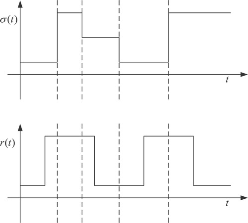
It is an apparent fact that the TRs of the Markov process determines the behaviour of the MSSs. Assuming that the considered model is a totally non-homogeneous MSS, then the corresponding problems are difficult to be explored. Hence, in this paper, the stochastic process $r\left(t\right)\in \mathcal{S}$ is assumed to be governed by a general homogeneous Markovian chain. To be more specific, the considered TRs are time-varying, but they are invariant during one interval. Hence, the considered time-varying TRs are more practical than the time-invariant TRs when dealing with the Markov process originated from practice. An illustration of this piecewise homogeneous evolution is shown in Figure 1.

Figure 1. Illustration of the piecewise-homogeneous evolution for systems with modes $r\left(t\right)\in \mathcal{S}=\{1,2\}$ and $\sigma \left(t\right)\in \mathcal{V}=\{1,2,3\}$.

For further discussion, the nonlinear functions concerned in (1(1) $\begin{array}{rl}\dot{z}\left(t\right)& =-C\left(r\right(t\left)\right)z\left(t\right)+A\left(r\right(t\left)\right)f\left(z\right(t\left)\right)\\ & +B\left(r\right(t\left)\right)g\left(z\right(t-{\tau }_{r\left(t\right),\sigma \left(t\right)}\left(t\right)\left)\right)+\tilde{u}\left(t\right),t\ge 0\end{array}$(1) ) are assumed to satisfy the following conditions.

Assumption 2.1

Let $\delta ={\delta }_1+\overrightarrow{\mathrm{i}}{\delta }_2$ with ${\delta }_1$, ${\delta }_2\in \mathbb{R}$. $f_{\upsilon }\left(\delta \right)$ and $g_{\upsilon }\left(\delta \right)$ can be represented by their real and imaginary parts with $\begin{array}{rl}{f}_{\upsilon }\left(\delta \right)& =f_{\upsilon }^R({\delta }_1,{\delta }_2)+\overrightarrow{\mathrm{i}}{f}_{\upsilon }^I({\delta }_1,{\delta }_2),\\ g_{\upsilon }\left(\delta \right)& =g_{\upsilon }^R({\delta }_1,{\delta }_2)+\overrightarrow{\mathrm{i}}{g}_{\upsilon }^I({\delta }_1,{\delta }_2)\end{array}$ where $\upsilon =1,2,\dots ,n$, and $f_{\upsilon }^R(\cdot )$, $f_{\upsilon }^I(\cdot )$, $g_{\upsilon }^R(\cdot )$, $g_{\upsilon }^I(\cdot ):{\mathbb{R}}^2\to \mathbb{R}$ satisfy $\begin{array}{rl}|f_{\upsilon }^R({\delta }_1,{\delta }_2)|& \le {\gamma }_{\upsilon }^{RR}|{\delta }_1|+{\gamma }_{\upsilon }^{RI}|{\delta }_2|,\\ |f_{\upsilon }^I({\delta }_1,{\delta }_2)|& \le {\gamma }_{\upsilon }^{IR}|{\delta }_1|+{\gamma }_{\upsilon }^{II}|{\delta }_2|,\\ |g_{\upsilon }^R({\delta }_1,{\delta }_2)|& \le {\varsigma }_{\upsilon }^{RR}|{\delta }_1|+{\varsigma }_{\upsilon }^{RI}|{\delta }_2|,\\ |g_{\upsilon }^I({\delta }_1,{\delta }_2)|& \le {\varsigma }_{\upsilon }^{IR}|{\delta }_1|+{\varsigma }_{\upsilon }^{II}|{\delta }_2|\end{array}$ in which ${\gamma }_{\upsilon }^{RR}$, ${\gamma }_{\upsilon }^{RI}$, ${\gamma }_{\upsilon }^{IR}$, ${\gamma }_{\upsilon }^{II}$, ${\varsigma }_{\upsilon }^{RR}$, ${\varsigma }_{\upsilon }^{RI}$, ${\varsigma }_{\upsilon }^{IR}$, and ${\varsigma }_{\upsilon }^{II}$ are known positive constants.

For ease discussion, denote ${\mathrm{{\rm Y}}}^{RR}\triangleq \mathrm{d}\mathrm{i}\mathrm{a}\mathrm{g}\{{\gamma }_{\upsilon }^{RR}{\}}_{\upsilon =1}^n$, ${\mathrm{{\rm Y}}}^{RI}\triangleq \mathrm{d}\mathrm{i}\mathrm{a}\mathrm{g}\{{\gamma }_{\upsilon }^{RI}{\}}_{\upsilon =1}^n$, ${\mathrm{{\rm Y}}}^{IR}\triangleq \mathrm{d}\mathrm{i}\mathrm{a}\mathrm{g}\{{\gamma }_{\upsilon }^{IR}{\}}_{\upsilon =1}^n$, ${\mathrm{{\rm Y}}}^{II}\triangleq \mathrm{d}\mathrm{i}\mathrm{a}\mathrm{g}\{{\gamma }_{\upsilon }^{II}{\}}_{\upsilon =1}^n$, ${\mathrm{\Psi }}^{RR}\triangleq \mathrm{d}\mathrm{i}\mathrm{a}\mathrm{g}\{{\varsigma }_{\upsilon }^{RR}{\}}_{\upsilon =1}^n$, ${\mathrm{\Psi }}^{RI}\triangleq \mathrm{d}\mathrm{i}\mathrm{a}\mathrm{g}\{{\varsigma }_{\upsilon }^{RI}{\}}_{\upsilon =1}^n$, ${\mathrm{\Psi }}^{IR}\triangleq \mathrm{d}\mathrm{i}\mathrm{a}\mathrm{g}\{{\varsigma }_{\upsilon }^{IR}{\}}_{\upsilon =1}^n$ and ${\mathrm{\Psi }}^{II}\triangleq \mathrm{d}\mathrm{i}\mathrm{a}\mathrm{g}\{{\varsigma }_{\upsilon }^{II}{\}}_{\upsilon =1}^n$ in the sequel.

For simplicity, when $r\left(t\right)=i$ and $\sigma \left(t\right)=m$, denote $A\left(r\right(t\left)\right)$ as $A_i=A_i^R+\overrightarrow{\mathrm{i}}{A}_i^I$, and the other symbols have the similar meanings which are omitted for space consideration if no confusion arises. Let $z\left(t\right)=x\left(t\right)+\overrightarrow{\mathrm{i}}y\left(t\right)$ with $x\left(t\right)=\mathrm{c}\mathrm{o}\mathrm{l}\left(x_{\upsilon }\right(t){)}_{\upsilon =1}^n$, $y\left(t\right)=\mathrm{c}\mathrm{o}\mathrm{l}\left(y_{\upsilon }\right(t){)}_{\upsilon =1}^n\in {\mathbb{R}}^n$, then system (1(1) $\begin{array}{rl}\dot{z}\left(t\right)& =-C\left(r\right(t\left)\right)z\left(t\right)+A\left(r\right(t\left)\right)f\left(z\right(t\left)\right)\\ & +B\left(r\right(t\left)\right)g\left(z\right(t-{\tau }_{r\left(t\right),\sigma \left(t\right)}\left(t\right)\left)\right)+\tilde{u}\left(t\right),t\ge 0\end{array}$(1) ) can be rewritten as follows: (5) $\begin{array}{rl}\dot{x}\left(t\right)& =-C_{i}x\left(t\right)+A_i^R{f}^R\left(x\right(t),y(t\left)\right)-A_i^I{f}^I\left(x\right(t),y(t\left)\right)\\ & +{\tilde{u}}^R\left(t\right)-B_i^I{g}^I\left(x\right(t-{\tau }_{i,m}\left(t\right)),y(t-{\tau }_{i,m}\left(t\right)\left)\right)\\ & +B_i^R{g}^R\left(x\right(t-{\tau }_{i,m}\left(t\right)),y(t-{\tau }_{i,m}\left(t\right)\left)\right),\\ \dot{y}\left(t\right)& =-C_{i}y\left(t\right)+A_i^R{f}^I\left(x\right(t),y(t\left)\right)+A_i^I{f}^R\left(x\right(t),y(t\left)\right)\\ & +{\tilde{u}}^I\left(t\right)+B_i^R{g}^I\left(x\right(t-{\tau }_{i,m}\left(t\right)),y(t-{\tau }_{i,m}\left(t\right)\left)\right)\\ & +B_i^I{g}^R\left(x\right(t-{\tau }_{i,m}\left(t\right)),y(t-{\tau }_{i,m}\left(t\right)\left)\right)\end{array}$(5) or in a more compact form: (6) $\begin{array}{rl}\dot{\xi }\left(t\right)& =-C_{1i}\xi \left(t\right)+A_{1i}{f}_1\left(\xi \right(t\left)\right)+A_{2i}{f}_2\left(\xi \right(t\left)\right)+u\left(t\right)\\ & +B_{1i}{g}_1\left(\xi \right(t-{\tau }_{i,m}\left(t\right)\left)\right)+B_{2i}{g}_2\left(\xi \right(t-{\tau }_{i,m}\left(t\right)\left)\right)\end{array}$(6) where $\begin{array}{rl}\xi \left(t\right)& =\left(x^{\mathrm{T}}\right(t),y^{\mathrm{T}}(t){)}^{\mathrm{T}},u(t)=(\left({\tilde{u}}^R\right(t){)}^{\mathrm{T}},({\tilde{u}}^I\left(t\right){)}^{\mathrm{T}}{)}^{\mathrm{T}},\\ f_1\left(\xi \right(t\left)\right)& =I_2\otimes f^R\left(x\right(t),y(t\left)\right),A_{1i}=\mathrm{d}\mathrm{i}\mathrm{a}\mathrm{g}\{A_i^R,A_i^I\},\\ f^R\left(x\right(t),y(t\left)\right)& =\mathrm{c}\mathrm{o}\mathrm{l}\left(f_{\upsilon }^R\right(x_{\upsilon }\left(t\right),y_{\upsilon }\left(t\right)){)}_{\upsilon =1}^n,C_{1i}=I_2\otimes C_i,\\ f_2\left(\xi \right(t\left)\right)& =I_2\otimes f^I\left(x\right(t),y(t\left)\right),A_{2i}=\mathrm{d}\mathrm{i}\mathrm{a}\mathrm{g}\{-A_i^I,A_i^R\},\\ f^I\left(x\right(t),y(t\left)\right)& =\mathrm{c}\mathrm{o}\mathrm{l}\left(f_{\upsilon }^I\right(x_{\upsilon }\left(t\right),y_{\upsilon }\left(t\right)){)}_{\upsilon =1}^n,\\ g_1\left(\xi \right(t\left)\right)& =I_2\otimes g^R\left(x\right(t),y(t\left)\right),B_{1i}=\mathrm{d}\mathrm{i}\mathrm{a}\mathrm{g}\{B_i^R,B_i^I\},\\ g^R\left(x\right(t),y(t\left)\right)& =\mathrm{c}\mathrm{o}\mathrm{l}\left(g_{\upsilon }^R\right(x_{\upsilon }\left(t\right),y_{\upsilon }\left(t\right)){)}_{\upsilon =1}^n,\\ g_2\left(\xi \right(t\left)\right)& =I_2\otimes g^I\left(x\right(t),y(t\left)\right),B_{2i}=\mathrm{d}\mathrm{i}\mathrm{a}\mathrm{g}\{-B_i^I,B_i^R\},\\ g^I\left(x\right(t),y(t\left)\right)& =\mathrm{c}\mathrm{o}\mathrm{l}\left(g_{\upsilon }^I\right(x_{\upsilon }\left(t\right),y_{\upsilon }\left(t\right)){)}_{\upsilon =1}^n.\end{array}$ The initial condition for system (6(6) $\begin{array}{rl}\dot{\xi }\left(t\right)& =-C_{1i}\xi \left(t\right)+A_{1i}{f}_1\left(\xi \right(t\left)\right)+A_{2i}{f}_2\left(\xi \right(t\left)\right)+u\left(t\right)\\ & +B_{1i}{g}_1\left(\xi \right(t-{\tau }_{i,m}\left(t\right)\left)\right)+B_{2i}{g}_2\left(\xi \right(t-{\tau }_{i,m}\left(t\right)\left)\right)\end{array}$(6) ) is given by (7) $\xi \left(s\right)=\varphi \left(s\right),s\in [-{\tau }_2,0]$(7) where $\varphi (\cdot )\in L_{{\mathcal{F}}_0}^2\left(\right[-{\tau }_2,0],{\mathbb{R}}^{2n})$ and $L_{{\mathcal{F}}_0}^2\left(\right[-{\tau }_2,0],{\mathbb{R}}^{2n})$ is the family of all ${\mathcal{F}}_0$-measurable ${\mathbf{C}}^1\left(\right[-{\tau }_2,0],{\mathbb{R}}^{2n})$-valued random variables satisfying $\underset{s\in [-{\tau }_2,0]}{sup}max\left\{\mathbb{E}\right\{\parallel \varphi \left(s\right){\parallel }^2\},\mathbb{E}\parallel \dot{\varphi }(s\left){\parallel }^2\right\}\}<\mathrm{\infty }$, and it is further assumed that $\varphi (\cdot )$ is independent with the two-level Markov processes $r\left(t\right)$ and $\sigma \left(t\right)$.

In order to derive the main results of this paper, the following basic definitions and lemmas are introduced, which will be utilized later.

Definition 2.1

Given $\text{β}>0$, system (1(1) $\begin{array}{rl}\dot{z}\left(t\right)& =-C\left(r\right(t\left)\right)z\left(t\right)+A\left(r\right(t\left)\right)f\left(z\right(t\left)\right)\\ & +B\left(r\right(t\left)\right)g\left(z\right(t-{\tau }_{r\left(t\right),\sigma \left(t\right)}\left(t\right)\left)\right)+\tilde{u}\left(t\right),t\ge 0\end{array}$(1) ) with $\tilde{u}\left(t\right)\equiv 0$ is said to be β-exponentially mean-square stable if there exists positive constant $\alpha >0$ such that, for all $t\ge 0$, the following inequality holds for any initial condition in (7(7) $\xi \left(s\right)=\varphi \left(s\right),s\in [-{\tau }_2,0]$(7) ): (8) $\begin{array}{rl}\mathbb{E}\{\parallel \xi (t\left){\parallel }^2\right\}& \le \alpha {\mathrm{e}}^{-\text{β}t}\underset{-{\tau }_2\le \theta \le 0}{sup}max\left\{\mathbb{E}\right\{\parallel \varphi \left(\theta \right){\parallel }^2\},\\ & \mathbb{E}\{\parallel \dot{\varphi }(\theta \left){\parallel }^2\right\}\}.\end{array}$(8)

Definition 2.2

Given $\text{β}>0$, system (1(1) $\begin{array}{rl}\dot{z}\left(t\right)& =-C\left(r\right(t\left)\right)z\left(t\right)+A\left(r\right(t\left)\right)f\left(z\right(t\left)\right)\\ & +B\left(r\right(t\left)\right)g\left(z\right(t-{\tau }_{r\left(t\right),\sigma \left(t\right)}\left(t\right)\left)\right)+\tilde{u}\left(t\right),t\ge 0\end{array}$(1) ) is said to be β-exponentially mean-square stabilizable if there exists a suitable feedback control law $\tilde{u}\left(t\right)$ such that the closed-loop system (1(1) $\begin{array}{rl}\dot{z}\left(t\right)& =-C\left(r\right(t\left)\right)z\left(t\right)+A\left(r\right(t\left)\right)f\left(z\right(t\left)\right)\\ & +B\left(r\right(t\left)\right)g\left(z\right(t-{\tau }_{r\left(t\right),\sigma \left(t\right)}\left(t\right)\left)\right)+\tilde{u}\left(t\right),t\ge 0\end{array}$(1) ) is β-exponentially mean-square stable, where β is also called the decay rate.

Lemma 2.1

Park et al., 2011

Consider one system with differentiable state $z(\cdot )\in {\mathbb{R}}^n$ and delay $\tau \left(t\right)$ that satisfies $0<\tau \left(t\right)\le {\tau }_M$. For any matrices $X=X^{\mathrm{T}}\in {\mathbb{R}}^{n\times n}$ and $U\in {\mathbb{R}}^{n\times n}$ that satisfy $\left[\begin{array}{cc}X& U\\ U^{\mathrm{T}}& X\end{array}\right]\ge 0,$ the following inequality holds: $\begin{array}{rl}-{\tau }_M{\int }_{t-{\tau }_M}^t{\dot{z}}^{\mathrm{T}}\left(s\right)X\dot{z}\left(s\right)\mathrm{d}s& \le {\left[\begin{array}{c}z\left(t\right)\\ z(t-\tau (t\left)\right)\\ z(t-{\tau }_M)\end{array}\right]}^{\mathrm{T}}\\ & \times \left[\begin{array}{ccc}-X& X-U& U\\ \ast & \mathcal{U}& X-U\\ \ast & \ast & -X\end{array}\right]\\ & \times \left[\begin{array}{c}z\left(t\right)\\ z(t-\tau (t\left)\right)\\ z(t-{\tau }_M)\end{array}\right]\end{array}$ where $\mathcal{U}\triangleq -2X+U+U^{\mathrm{T}}$.

Lemma 2.2

Boyd et al., 1994

A given matrix $\overline{\mathrm{\Omega }}=\left[\begin{array}{cc}{\mathrm{\Omega }}_{11}& {\mathrm{\Omega }}_{12}\\ {\mathrm{\Omega }}_{21}& {\mathrm{\Omega }}_{22}\end{array}\right]<0,$ where ${\mathrm{\Omega }}_{11}^{\mathrm{T}}={\mathrm{\Omega }}_{11},{\mathrm{\Omega }}_{12}^{\mathrm{T}}={\mathrm{\Omega }}_{21}$ and ${\mathrm{\Omega }}_{22}^{\mathrm{T}}={\mathrm{\Omega }}_{22},$ is equivalent to any one of the following conditions:

1. ${\mathrm{\Omega }}_{22}<0$ and ${\mathrm{\Omega }}_{11}-{\mathrm{\Omega }}_{12}{\mathrm{\Omega }}_{22}^{-1}{\mathrm{\Omega }}_{21}<0,$

2. ${\mathrm{\Omega }}_{11}<0$ and ${\mathrm{\Omega }}_{22}-{\mathrm{\Omega }}_{21}{\mathrm{\Omega }}_{11}^{-1}{\mathrm{\Omega }}_{12}<0$.

3. Main results

In this section, we will establish our main results based on matrix inequality approach. The first one is for exponential stability of system (6(6) $\begin{array}{rl}\dot{\xi }\left(t\right)& =-C_{1i}\xi \left(t\right)+A_{1i}{f}_1\left(\xi \right(t\left)\right)+A_{2i}{f}_2\left(\xi \right(t\left)\right)+u\left(t\right)\\ & +B_{1i}{g}_1\left(\xi \right(t-{\tau }_{i,m}\left(t\right)\left)\right)+B_{2i}{g}_2\left(\xi \right(t-{\tau }_{i,m}\left(t\right)\left)\right)\end{array}$(6) ), and the other is for the stabilization of system (6(6) $\begin{array}{rl}\dot{\xi }\left(t\right)& =-C_{1i}\xi \left(t\right)+A_{1i}{f}_1\left(\xi \right(t\left)\right)+A_{2i}{f}_2\left(\xi \right(t\left)\right)+u\left(t\right)\\ & +B_{1i}{g}_1\left(\xi \right(t-{\tau }_{i,m}\left(t\right)\left)\right)+B_{2i}{g}_2\left(\xi \right(t-{\tau }_{i,m}\left(t\right)\left)\right)\end{array}$(6) ) by appropriately designing a mode-dependent Markovian switching control law.

Theorem 3.1

Under Assumption 2.1, for given $\text{β}>0,$ system (6(6) $\begin{array}{rl}\dot{\xi }\left(t\right)& =-C_{1i}\xi \left(t\right)+A_{1i}{f}_1\left(\xi \right(t\left)\right)+A_{2i}{f}_2\left(\xi \right(t\left)\right)+u\left(t\right)\\ & +B_{1i}{g}_1\left(\xi \right(t-{\tau }_{i,m}\left(t\right)\left)\right)+B_{2i}{g}_2\left(\xi \right(t-{\tau }_{i,m}\left(t\right)\left)\right)\end{array}$(6) ) is $2\text{β}$-exponentially stable in the mean square with $u\left(t\right)\equiv 0$ if there exist positive definite matrices $P_{i,m},$ Q, R, positive diagonal matrices $G_{\iota },$ $J_{\iota },$ matrices S, $Z_{i,m},$ $T_{i,m}$ with appropriate dimensions, and scalars ${\vartheta }_{\iota }>0(\iota =1,2,3,4)$ such that the following inequalities (9(9) $\begin{array}{rl}& {\mathrm{\Gamma }}_{\iota }\le G_{\iota },\end{array}$(9) )–(13(13) $\begin{array}{rl}& \left[\begin{array}{cccccc}& {\mathrm{\Xi }}_{11}& 0& 0& 0& P_{i,m}{A}_{1i}\\ \ast & {\mathrm{\Xi }}_{22}& {\mathrm{\Xi }}_{23}& S& 0& 0\\ \ast & \ast & {\mathrm{\Xi }}_{33}& {\mathrm{\Xi }}_{34}& 0& 0\\ \ast & \ast & \ast & {\mathrm{\Xi }}_{44}& 0& 0\\ \ast & \ast & \ast & \ast & {\mathrm{\Xi }}_{55}& 0\\ \ast & \ast & \ast & \ast & \ast & {\mathrm{\Xi }}_{66}\\ \ast & \ast & \ast & \ast & \ast & \ast \\ \ast & \ast & \ast & \ast & \ast & \ast \\ \ast & \ast & \ast & \ast & \ast & \ast \end{array}\right.\\ & \left.\begin{array}{cccc}{P}_{i,m}{A}_{2i}& P_{i,m}{B}_{1i}& P_{i,m}{B}_{2i}& -C_{1i}^{\mathrm{T}}{R}^{\ast }\\ 0& 0& 0& \\ 0& 0& 0& \\ 0& 0& 0& \\ 0& 0& A_{1i}^{\mathrm{T}}{R}^{\ast }& \\ 0& 0& A_{2i}^{\mathrm{T}}{R}^{\ast }& \\ {\mathrm{\Xi }}_{77}& 0& B_{1i}^{\mathrm{T}}{R}^{\ast }& \\ \ast & {\mathrm{\Xi }}_{88}& B_{2i}^{\mathrm{T}}{R}^{\ast }& \\ \ast & \ast & -R\end{array}\right]<0\end{array}$(13) ) hold for all $i\in \mathcal{S},$ $m\in \mathcal{V}$: (9) $\begin{array}{rl}& {\mathrm{\Gamma }}_{\iota }\le G_{\iota },\end{array}$(9) (10) $\begin{array}{rl}& \left[\begin{array}{cc}{\mathrm{e}}^{-2\text{β}{\tau }_2}R& S\\ \ast & {\mathrm{e}}^{-2\text{β}{\tau }_2}R\end{array}\right]>0,\end{array}$(10) (11) $\begin{array}{rl}& \left\{\begin{array}{ll}{P}_{j,m}-Z_{i,m}\le 0,& j\in {\mathcal{S}}_{uk}^i\mathrm{\setminus }\left\{i\right\}\\ P_{j,m}-Z_{i,m}\ge 0,& j\in {\mathcal{S}}_{uk}^i\cap \left\{i\right\}\end{array}\right.\end{array}$(11) (12) $\begin{array}{rl}& \left\{\begin{array}{ll}{P}_{i,n}-T_{i,m}\le 0,& n\in {\mathcal{V}}_{uk}^m\mathrm{\setminus }\left\{m\right\}\\ P_{i,n}-T_{i,m}\ge 0,& n\in {\mathcal{V}}_{uk}^m\cap \left\{m\right\}\end{array}\right.\end{array}$(12) (13) $\begin{array}{rl}& \left[\begin{array}{cccccc}& {\mathrm{\Xi }}_{11}& 0& 0& 0& P_{i,m}{A}_{1i}\\ \ast & {\mathrm{\Xi }}_{22}& {\mathrm{\Xi }}_{23}& S& 0& 0\\ \ast & \ast & {\mathrm{\Xi }}_{33}& {\mathrm{\Xi }}_{34}& 0& 0\\ \ast & \ast & \ast & {\mathrm{\Xi }}_{44}& 0& 0\\ \ast & \ast & \ast & \ast & {\mathrm{\Xi }}_{55}& 0\\ \ast & \ast & \ast & \ast & \ast & {\mathrm{\Xi }}_{66}\\ \ast & \ast & \ast & \ast & \ast & \ast \\ \ast & \ast & \ast & \ast & \ast & \ast \\ \ast & \ast & \ast & \ast & \ast & \ast \end{array}\right.\\ & \left.\begin{array}{cccc}{P}_{i,m}{A}_{2i}& P_{i,m}{B}_{1i}& P_{i,m}{B}_{2i}& -C_{1i}^{\mathrm{T}}{R}^{\ast }\\ 0& 0& 0& \\ 0& 0& 0& \\ 0& 0& 0& \\ 0& 0& A_{1i}^{\mathrm{T}}{R}^{\ast }& \\ 0& 0& A_{2i}^{\mathrm{T}}{R}^{\ast }& \\ {\mathrm{\Xi }}_{77}& 0& B_{1i}^{\mathrm{T}}{R}^{\ast }& \\ \ast & {\mathrm{\Xi }}_{88}& B_{2i}^{\mathrm{T}}{R}^{\ast }& \\ \ast & \ast & -R\end{array}\right]<0\end{array}$(13) in which $R^{\ast }=({\tau }_2-{\tau }_1)R$, ${\mathrm{\Xi }}_{22}=-{\mathrm{e}}^{-2\text{β}{\tau }_2}R,$ ${\mathrm{\Xi }}_{23}={\mathrm{\Xi }}_{34}={\mathrm{e}}^{-2\text{β}{\tau }_2}R-S,$ ${\mathrm{\Xi }}_{44}=-{\mathrm{e}}^{-2\text{β}{\tau }_2}R,$ $\begin{array}{rl}{\mathrm{\Xi }}_{11}& =2\text{β}{P}_{i,m}-P_{i,m}{C}_{1i}-C_{1i}{P}_{i,m}+Q\\ & +(\overline{\lambda }+\overline{\pi })({\tau }_2-{\tau }_1)Q+2{\vartheta }_1{G}_1+2{\vartheta }_2{G}_2\\ & +\sum _{j\in {\mathcal{S}}_k^i}{\lambda }_{ij}^m(P_{j,m}-Z_{i,m})+\sum _{n\in {\mathcal{V}}_k^m}{\pi }_{mn}(P_{i,n}-T_{i,m}),\\ {\mathrm{\Xi }}_{33}& =-(1-\overline{\tau }){\mathrm{e}}^{-2\text{β}\ell }Q-2{\mathrm{e}}^{-2\text{β}{\tau }_2}R+S+S^{\mathrm{T}}\\ & +2{\vartheta }_3{G}_3+2{\vartheta }_4{G}_4,\\ {\mathrm{\Xi }}_{55}& =-{\vartheta }_1(I_2\otimes J_1),{\mathrm{\Xi }}_{66}=-{\vartheta }_2(I_2\otimes J_2),\\ {\mathrm{\Xi }}_{77}& =-{\vartheta }_3(I_2\otimes J_3),{\mathrm{\Xi }}_{88}=-{\vartheta }_4(I_2\otimes J_4)\end{array}$ with $\begin{array}{rl}& {\mathrm{\Gamma }}_1=\left(\begin{array}{cc}{J}_1({\mathrm{{\rm Y}}}^{RR}{)}^2& J_1{\mathrm{{\rm Y}}}^{RR}{\mathrm{{\rm Y}}}^{RI}\\ J_1{\mathrm{{\rm Y}}}^{RR}{\mathrm{{\rm Y}}}^{RI}& J_1({\mathrm{{\rm Y}}}^{RI}{)}^2\end{array}\right),\\ & {\mathrm{\Gamma }}_2=\left(\begin{array}{cc}{J}_2({\mathrm{{\rm Y}}}^{IR}{)}^2& J_2{\mathrm{{\rm Y}}}^{II}{\mathrm{{\rm Y}}}^{RI}\\ J_2{\mathrm{{\rm Y}}}^{IR}{\mathrm{{\rm Y}}}^{II}& J_2({\mathrm{{\rm Y}}}^{II}{)}^2\end{array}\right),\\ & {\mathrm{\Gamma }}_3=\left(\begin{array}{cc}{J}_3({\mathrm{\Psi }}^{RR}{)}^2& J_3{\mathrm{\Psi }}^{RR}{\mathrm{\Psi }}^{RI}\\ J_3{\mathrm{\Psi }}^{RR}{\mathrm{\Psi }}^{RI}& J_3({\mathrm{\Psi }}^{RI}{)}^2\end{array}\right),\\ & {\mathrm{\Gamma }}_4=\left(\begin{array}{cc}{J}_4({\mathrm{\Psi }}^{IR}{)}^2& J_4{\mathrm{\Psi }}^{II}{\mathrm{\Psi }}^{RI}\\ J_4{\mathrm{\Psi }}^{IR}{\mathrm{\Psi }}^{II}& J_4({\mathrm{\Psi }}^{II}{)}^2\end{array}\right)\end{array}$ and $\ell ={\tau }_2$ when $\overline{\tau }<1,$ and $\ell ={\tau }_1$ when $\overline{\tau }\ge 1$.

Proof.

Construct the following appropriate Lyapunov–Krasovskii functional candidate for system (6(6) $\begin{array}{rl}\dot{\xi }\left(t\right)& =-C_{1i}\xi \left(t\right)+A_{1i}{f}_1\left(\xi \right(t\left)\right)+A_{2i}{f}_2\left(\xi \right(t\left)\right)+u\left(t\right)\\ & +B_{1i}{g}_1\left(\xi \right(t-{\tau }_{i,m}\left(t\right)\left)\right)+B_{2i}{g}_2\left(\xi \right(t-{\tau }_{i,m}\left(t\right)\left)\right)\end{array}$(6) ): (14) $\overline{V}(t,\xi (t),r(t),\sigma (t\left)\right)=\sum _{\iota =1}^4{\overline{V}}_{\iota }(t,\xi (t),r(t),\sigma (t\left)\right)$(14) where $\begin{array}{rl}{\overline{V}}_1(t,\xi (t),r(t),\sigma (t\left)\right)& ={\mathrm{e}}^{2\text{β}t}{\xi }^{\mathrm{T}}\left(t\right)P_{r\left(t\right),\sigma \left(t\right)}\xi \left(t\right),\\ {\overline{V}}_2(t,\xi (t),r(t),\sigma (t\left)\right)& ={\int }_{t-{\tau }_{r\left(t\right),\sigma \left(t\right)}\left(t\right)}^t{\mathrm{e}}^{2\text{β}s}{\xi }^{\mathrm{T}}\left(s\right)Q\xi \left(s\right)\mathrm{d}s,\\ {\overline{V}}_3(t,\xi (t),r(t),\sigma (t\left)\right)& =(\overline{\lambda }+\overline{\pi }){\int }_{{\tau }_1}^{{\tau }_2}\\ & \times {\int }_{t-s}^t{\mathrm{e}}^{2\text{β}\theta }{\xi }^{\mathrm{T}}\left(\theta \right)Q\xi \left(\theta \right)\mathrm{d}\theta \mathrm{d}s,\\ {\overline{V}}_4(t,\xi (t),r(t),\sigma (t\left)\right)& =({\tau }_2-{\tau }_1){\int }_{{\tau }_1}^{{\tau }_2}\\ & \times {\int }_{t-s}^t{\mathrm{e}}^{2\text{β}\theta }{\dot{\xi }}^{\mathrm{T}}\left(\theta \right)R\dot{\xi }\left(\theta \right)\mathrm{d}\theta \mathrm{d}s\end{array}$ in which $P_{r\left(t\right),\sigma \left(t\right)}$, Q, and R are matrices to be determined.

Let $\mathcal{L}$ be the infinitesimal generator acting on $\overline{V}(t,\xi (t),r(t),\sigma (t\left)\right)$. According to the definition of $\mathcal{L}$ (Dynkin, 1965), when $r\left(t\right)=i$ and $\sigma \left(t\right)=m$, equality (15(15) $\begin{array}{rl}& \mathcal{L}\overline{V}(t,\xi (t),i,m)=\underset{h\to 0^{+}}{lim}\frac{\begin{array}{c}\mathbb{E}\left\{\overline{V}\right(t+h,\xi (t+h),r(t+h),\\ \sigma (t+h)\left)|\xi \right(t),r(t)=i,\\ \sigma \left(t\right)=m\}-\overline{V}(t,\xi \left(t\right),i,m)\end{array}}{h}\\ & =\underset{h\to 0^{+}}{lim}\frac{1}{h}\left\{\sum _{n\in \mathcal{V}\mathrm{\setminus }\left\{m\right\}}{\pi }_{mn}h\left[\sum _{j\in \mathcal{S}\mathrm{\setminus }\left\{i\right\}}{\lambda }_{ij}^{n}h\overline{V}(t+h,\xi (t+h),\right.\right.\\ & \left.j,n)+(1+{\lambda }_{ii}^{n}h\left)\overline{V}\right(t+h,\xi (t+h),i,n)\phantom{\sum _{n\in \mathcal{V}\mathrm{\setminus }\left\{m\right\}}}\right]\\ & +(1+{\pi }_{mm}h)\left[\sum _{j\in \mathcal{S}\mathrm{\setminus }\left\{i\right\}}{\lambda }_{ij}^{m}h\overline{V}(t+h,\xi (t+h),j,m)\right.\\ & \left.\phantom{\sum _{n\in \mathcal{V}\mathrm{\setminus }\left\{m\right\}}}+(1+{\lambda }_{ii}^{m}h)\overline{V}(t+h,\xi (t+h),i,m)\right]\\ & \left.\phantom{\sum _{n\in \mathcal{V}\mathrm{\setminus }\left\{m\right\}}}-\overline{V}(t,\xi (t),i,m)\right\}\\ & =\underset{h\to 0^{+}}{lim}\frac{1}{h}\left\{\sum _{n\in \mathcal{V}\mathrm{\setminus }\left\{m\right\}}{\pi }_{mn}h\overline{V}(t+h,\xi (t+h),i,n)\right.\\ & +{\pi }_{mn}h\overline{V}(t+h,\xi (t+h),i,m)\\ & +\left[\sum _{j\in \mathcal{S}\mathrm{\setminus }\left\{i\right\}}{\lambda }_{ij}^{m}h\overline{V}(t+h,\xi (t+h),j,m)\right.\\ & \left.+(1+{\lambda }_{ii}^{m}h)\overline{V}(t+h,\xi (t+h),i,m)\phantom{\sum _{n\in \mathcal{V}\mathrm{\setminus }\left\{m\right\}}}\right]\\ & \left.\phantom{\sum _{n\in \mathcal{V}\mathrm{\setminus }\left\{m\right\}}}-\overline{V}(t,\xi (t),i,m)\right\}\\ & =\underset{h\to 0^{+}}{lim}\frac{1}{h}\{\sum _{n\in \mathcal{V}}{\pi }_{mn}h\overline{V}(t+h,\xi (t+h),i,n)\\ & +\sum _{j\in \mathcal{S}}{\lambda }_{ij}^{m}h\overline{V}(t+h,\xi (t+h),j,m)\\ & +[\overline{V}(t+h,\xi (t+h),i,m)-\overline{V}(t,\xi (t),i,m)]\}\\ & =\sum _{n\in \mathcal{V}}{\pi }_{mn}\overline{V}(t,\xi (t),i,n)+\sum _{j\in \mathcal{S}}{\lambda }_{ij}^m\overline{V}(t,\xi (t),j,m)\\ & +\dot{\overline{V}}(t,\xi (t),i,m).\end{array}$(15) ) can be derived. (15) $\begin{array}{rl}& \mathcal{L}\overline{V}(t,\xi (t),i,m)=\underset{h\to 0^{+}}{lim}\frac{\begin{array}{c}\mathbb{E}\left\{\overline{V}\right(t+h,\xi (t+h),r(t+h),\\ \sigma (t+h)\left)|\xi \right(t),r(t)=i,\\ \sigma \left(t\right)=m\}-\overline{V}(t,\xi \left(t\right),i,m)\end{array}}{h}\\ & =\underset{h\to 0^{+}}{lim}\frac{1}{h}\left\{\sum _{n\in \mathcal{V}\mathrm{\setminus }\left\{m\right\}}{\pi }_{mn}h\left[\sum _{j\in \mathcal{S}\mathrm{\setminus }\left\{i\right\}}{\lambda }_{ij}^{n}h\overline{V}(t+h,\xi (t+h),\right.\right.\\ & \left.j,n)+(1+{\lambda }_{ii}^{n}h\left)\overline{V}\right(t+h,\xi (t+h),i,n)\phantom{\sum _{n\in \mathcal{V}\mathrm{\setminus }\left\{m\right\}}}\right]\\ & +(1+{\pi }_{mm}h)\left[\sum _{j\in \mathcal{S}\mathrm{\setminus }\left\{i\right\}}{\lambda }_{ij}^{m}h\overline{V}(t+h,\xi (t+h),j,m)\right.\\ & \left.\phantom{\sum _{n\in \mathcal{V}\mathrm{\setminus }\left\{m\right\}}}+(1+{\lambda }_{ii}^{m}h)\overline{V}(t+h,\xi (t+h),i,m)\right]\\ & \left.\phantom{\sum _{n\in \mathcal{V}\mathrm{\setminus }\left\{m\right\}}}-\overline{V}(t,\xi (t),i,m)\right\}\\ & =\underset{h\to 0^{+}}{lim}\frac{1}{h}\left\{\sum _{n\in \mathcal{V}\mathrm{\setminus }\left\{m\right\}}{\pi }_{mn}h\overline{V}(t+h,\xi (t+h),i,n)\right.\\ & +{\pi }_{mn}h\overline{V}(t+h,\xi (t+h),i,m)\\ & +\left[\sum _{j\in \mathcal{S}\mathrm{\setminus }\left\{i\right\}}{\lambda }_{ij}^{m}h\overline{V}(t+h,\xi (t+h),j,m)\right.\\ & \left.+(1+{\lambda }_{ii}^{m}h)\overline{V}(t+h,\xi (t+h),i,m)\phantom{\sum _{n\in \mathcal{V}\mathrm{\setminus }\left\{m\right\}}}\right]\\ & \left.\phantom{\sum _{n\in \mathcal{V}\mathrm{\setminus }\left\{m\right\}}}-\overline{V}(t,\xi (t),i,m)\right\}\\ & =\underset{h\to 0^{+}}{lim}\frac{1}{h}\{\sum _{n\in \mathcal{V}}{\pi }_{mn}h\overline{V}(t+h,\xi (t+h),i,n)\\ & +\sum _{j\in \mathcal{S}}{\lambda }_{ij}^{m}h\overline{V}(t+h,\xi (t+h),j,m)\\ & +[\overline{V}(t+h,\xi (t+h),i,m)-\overline{V}(t,\xi (t),i,m)]\}\\ & =\sum _{n\in \mathcal{V}}{\pi }_{mn}\overline{V}(t,\xi (t),i,n)+\sum _{j\in \mathcal{S}}{\lambda }_{ij}^m\overline{V}(t,\xi (t),j,m)\\ & +\dot{\overline{V}}(t,\xi (t),i,m).\end{array}$(15) Therefore, it is straightforward to obtain that (16a) $\begin{array}{rl}\mathcal{L}{\overline{V}}_1(t,\xi (t),i,m)& =2\text{β}{\mathrm{e}}^{2\text{β}t}{\xi }^{\mathrm{T}}\left(t\right)P_{i,m}\xi \left(t\right)\\ & +2{\mathrm{e}}^{2\text{β}t}{\xi }^{\mathrm{T}}\left(t\right)P_{i,m}\dot{\xi }\left(t\right)\\ & +{\mathrm{e}}^{2\text{β}t}{\xi }^{\mathrm{T}}\left(t\right)\\ & \times \left\{\sum _{j\in \mathcal{S}}{\lambda }_{ij}^m{P}_{j,m}+\sum _{n\in \mathcal{V}}{\pi }_{mn}{P}_{i,n}\right\}\xi \left(t\right),\end{array}$(16a) (16b) $\begin{array}{rl}\mathcal{L}{\overline{V}}_2(t,\xi (t),i,m)& ={\mathrm{e}}^{2\text{β}t}{\xi }^{\mathrm{T}}\left(t\right)Q\xi \left(t\right)\\ & -(1-{\dot{\tau }}_{i,m}(t\left)\right){\mathrm{e}}^{2\text{β}(t-{\tau }_{i,m}(t\left)\right)}\\ & \times {\xi }^{\mathrm{T}}(t-{\tau }_{i,m}(t\left)\right)Q\xi (t-{\tau }_{i,m}(t\left)\right)\\ & +\sum _{j\in \mathcal{S}}{\lambda }_{ij}^m{\int }_{t-{\tau }_{j,m}\left(t\right)}^t{\mathrm{e}}^{2\text{β}s}{\xi }^{\mathrm{T}}\left(s\right)Q\xi \left(s\right)\mathrm{d}s\\ & +\sum _{n\in \mathcal{V}}{\pi }_{mn}{\int }_{t-{\tau }_{i,n}\left(t\right)}^t{\mathrm{e}}^{2\text{β}s}{\xi }^{\mathrm{T}}\left(s\right)Q\xi \left(s\right)\mathrm{d}s\\ & \le {\mathrm{e}}^{2\text{β}t}{\xi }^{\mathrm{T}}\left(t\right)Q\xi \left(t\right)-(1-\overline{\tau }){\mathrm{e}}^{2\text{β}(t-{\tau }_{i,m}(t\left)\right)}\\ & \times {\xi }^{\mathrm{T}}(t-{\tau }_{i,m}(t\left)\right)Q\xi (t-{\tau }_{i,m}(t\left)\right)\\ & +\sum _{j\in \mathcal{S}}{\lambda }_{ij}^m{\int }_{t-{\tau }_{j,m}\left(t\right)}^t{\mathrm{e}}^{2\text{β}s}{\xi }^{\mathrm{T}}\left(s\right)Q\xi \left(s\right)\mathrm{d}s\\ & +\sum _{n\in \mathcal{V}}{\pi }_{mn}{\int }_{t-{\tau }_{i,n}\left(t\right)}^t{\mathrm{e}}^{2\text{β}s}{\xi }^{\mathrm{T}}\left(s\right)Q\xi \left(s\right)\mathrm{d}s,\end{array}$(16b) (16c) $\begin{array}{rl}\mathcal{L}{\overline{V}}_3(t,\xi (t),i,m)& =(\overline{\lambda }+\overline{\pi })({\tau }_2-{\tau }_1){\mathrm{e}}^{2\text{β}t}{\xi }^{\mathrm{T}}\left(t\right)Q\xi \left(t\right)\\ & -(\overline{\lambda }+\overline{\pi }){\int }_{t-{\tau }_2}^{t-{\tau }_1}{\mathrm{e}}^{2\text{β}s}{\xi }^{\mathrm{T}}\left(s\right)Q\xi \left(s\right)\mathrm{d}s,\end{array}$(16c) (16d) $\begin{array}{rl}\mathcal{L}{\overline{V}}_4(t,\xi (t),i,m)& =({\tau }_2-{\tau }_1{)}^2{\mathrm{e}}^{2\text{β}t}{\dot{\xi }}^{\mathrm{T}}(t\left)R\dot{\xi }\right(t)\\ & -({\tau }_2-{\tau }_1){\int }_{t-{\tau }_2}^{t-{\tau }_1}{\mathrm{e}}^{2\text{β}s}{\dot{\xi }}^{\mathrm{T}}\left(s\right)R\dot{\xi }\left(s\right)\mathrm{d}s.\end{array}$(16d) According to the characteristics of TR matrices ${\mathrm{\Lambda }}^{\sigma (t+\mathrm{\Delta }t)}=[{\lambda }_{ij}^{\sigma (t+\mathrm{\Delta }t)}{]}_{N\times N}$ and $\mathrm{\Pi }=[{\pi }_{mn}{]}_{M\times M}$, for any mode-dependent matrices $Z_{i,m}$ and $T_{i,m}$, the following equalities hold: (17a) $\begin{array}{rl}& {\xi }^{\mathrm{T}}\left(t\right)\left\{\sum _{j\in \mathcal{S}}{\lambda }_{ij}^m{Z}_{i,m}\right\}\xi \left(t\right)\\ & ={\xi }^{\mathrm{T}}\left(t\right)\left\{\sum _{j\in {\mathcal{S}}_k^i}{\lambda }_{ij}^m{Z}_{i,m}+\sum _{j\in {\mathcal{S}}_{uk}^i}{\lambda }_{ij}^m{Z}_{i,m}\right\}\xi \left(t\right)=0,\end{array}$(17a) (17b) $\begin{array}{rl}& {\xi }^{\mathrm{T}}\left(t\right)\left\{\sum _{n\in \mathcal{V}}{\pi }_{mn}{T}_{i,m}\right\}\xi \left(t\right)\\ & ={\xi }^{\mathrm{T}}\left(t\right)\left\{\sum _{n\in {\mathcal{V}}_k^m}{\pi }_{mn}{T}_{i,m}+\sum _{n\in {\mathcal{V}}_{uk}^m}{\pi }_{mn}{T}_{i,m}\right\}\xi \left(t\right)=0.\end{array}$(17b) Moreover, it follows from $\overline{\pi }=\underset{1\le i\le M}{max}\{-{\pi }_{ii}\}$ and $\overline{\lambda }=\underset{m\in \mathcal{V}}{max}\underset{1\le i\le N}{max}\{-{\lambda }_{ii}^m\}$ that (18a) $\begin{array}{rl}& \sum _{j\in \mathcal{S}}{\lambda }_{ij}^m{\int }_{t-{\tau }_{j,m}\left(t\right)}^t{\mathrm{e}}^{2\text{β}s}{\xi }^{\mathrm{T}}\left(s\right)Q\xi \left(s\right)\mathrm{d}s\\ & =\sum _{j\in \mathcal{S}\mathrm{\setminus }\left\{i\right\}}{\lambda }_{ij}^m{\int }_{t-{\tau }_{j,m}\left(t\right)}^t{\mathrm{e}}^{2\text{β}s}{\xi }^{\mathrm{T}}\left(s\right)Q\xi \left(s\right)\mathrm{d}s\\ & +{\lambda }_{ii}^m{\int }_{t-{\tau }_{i,m}\left(t\right)}^t{\mathrm{e}}^{2\text{β}s}{\xi }^{\mathrm{T}}\left(s\right)Q\xi \left(s\right)\mathrm{d}s\\ & \le \sum _{j\in \mathcal{S}\mathrm{\setminus }\left\{i\right\}}{\lambda }_{ij}^m{\int }_{t-{\tau }_2}^t{\mathrm{e}}^{2\text{β}s}{\xi }^{\mathrm{T}}\left(s\right)Q\xi \left(s\right)\mathrm{d}s\\ & +{\lambda }_{ii}^m{\int }_{t-{\tau }_1}^t{\mathrm{e}}^{2\text{β}s}{\xi }^{\mathrm{T}}\left(s\right)Q\xi \left(s\right)\mathrm{d}s\\ & \le \overline{\lambda }{\int }_{t-{\tau }_2}^{t-{\tau }_1}{\mathrm{e}}^{2\text{β}s}{\xi }^{\mathrm{T}}\left(s\right)Q\xi \left(s\right)\mathrm{d}s,\end{array}$(18a) (18b) $\begin{array}{rl}& \sum _{n\in \mathcal{V}}{\pi }_{mn}{\int }_{t-{\tau }_{j,n}\left(t\right)}^t{\mathrm{e}}^{2\text{β}s}{\xi }^{\mathrm{T}}\left(s\right)Q\xi \left(s\right)\mathrm{d}s\\ & =\sum _{n\in \mathcal{V}\mathrm{\setminus }\left\{m\right\}}{\pi }_{mn}{\int }_{t-{\tau }_{i,n}\left(t\right)}^t{\mathrm{e}}^{2\text{β}s}{\xi }^{\mathrm{T}}\left(s\right)Q\xi \left(s\right)\mathrm{d}s\\ & +{\pi }_{mm}{\int }_{t-{\tau }_{i,m}\left(t\right)}^t{\mathrm{e}}^{2\text{β}s}{\xi }^{\mathrm{T}}\left(s\right)Q\xi \left(s\right)\mathrm{d}s\\ & \le \sum _{n\in \mathcal{V}\mathrm{\setminus }\left\{m\right\}}{\pi }_{mn}{\int }_{t-{\tau }_2}^t{\mathrm{e}}^{2\text{β}s}{\xi }^{\mathrm{T}}\left(s\right)Q\xi \left(s\right)\mathrm{d}s\\ & +{\pi }_{mm}{\int }_{t-{\tau }_1}^t{\mathrm{e}}^{2\text{β}s}{\xi }^{\mathrm{T}}\left(s\right)Q\xi \left(s\right)\mathrm{d}s\\ & \le \overline{\pi }{\int }_{t-{\tau }_2}^{t-{\tau }_1}{\mathrm{e}}^{2\text{β}s}{\xi }^{\mathrm{T}}\left(s\right)Q\xi \left(s\right)\mathrm{d}s.\end{array}$(18b) In term of Lemma 2.1, for any matrix S satisfying (10(10) $\begin{array}{rl}& \left[\begin{array}{cc}{\mathrm{e}}^{-2\text{β}{\tau }_2}R& S\\ \ast & {\mathrm{e}}^{-2\text{β}{\tau }_2}R\end{array}\right]>0,\end{array}$(10) ), it is easy to obtain (19) $\begin{array}{rl}& -({\tau }_2-{\tau }_1){\int }_{t-{\tau }_2}^{t-{\tau }_1}{\mathrm{e}}^{2\text{β}s}{\dot{\xi }}^{\mathrm{T}}\left(s\right)R\dot{\xi }\left(s\right)\mathrm{d}s\\ & \le -({\tau }_2-{\tau }_1){\mathrm{e}}^{2\text{β}t}{\int }_{t-{\tau }_2}^{t-{\tau }_1}{\dot{\xi }}^{\mathrm{T}}\left(s\right){\mathrm{e}}^{-2\text{β}{\tau }_2}R\dot{\xi }\left(s\right)\mathrm{d}s\\ & \le {\mathrm{e}}^{2\text{β}t}{\varpi }^{\mathrm{T}}\left(t\right)\mathrm{\Omega }\varpi \left(t\right)\end{array}$(19) where $\varpi \left(t\right)\triangleq \left[{\xi }^{\mathrm{T}}\right(t-{\tau }_2),{\xi }^{\mathrm{T}}(t-{\tau }_{i,m}\left(t\right)),{\xi }^{\mathrm{T}}(t-{\tau }_1){]}^{\mathrm{T}}$, and $\mathrm{\Omega }=\left[\begin{array}{ccc}-{\mathrm{e}}^{-2\text{β}{\tau }_2}R& {\mathrm{e}}^{-2\text{β}{\tau }_2}R-S& S\\ \ast & -2{\mathrm{e}}^{-2\text{β}{\tau }_2}R+S+S^{\mathrm{T}}& -S+{\mathrm{e}}^{-2\text{β}{\tau }_2}R\\ \ast & \ast & -{\mathrm{e}}^{-2\text{β}{\tau }_2}R\end{array}\right].$ On the other hand, by utilizing Assumption 2.1, one has $\begin{array}{rl}& f_1^{\mathrm{T}}\left(\xi \right(t\left)\right)(I_2\otimes J_1)f_1\left(\xi \right(t\left)\right)\\ & =2\sum _{k=1}^n{\mu }_{1k}\left(f_k^R\right(x_k\left(t\right),y_k\left(t\right)){)}^2\\ & \le 2\sum _{k=1}^n{\left(\begin{array}{c}|x_k\left(t\right)|\\ |y_k\left(t\right)|\end{array}\right)}^{\mathrm{T}}\left(\begin{array}{cc}{\mu }_{1k}({\gamma }_k^{RR}{)}^2& {\mu }_{1k}{\gamma }_k^{RR}{\gamma }_k^{RI}\\ {\mu }_{1k}{\gamma }_k^{RR}{\gamma }_k^{RI}& {\mu }_{1k}({\gamma }_k^{RI}{)}^2\end{array}\right)\left(\begin{array}{c}|x_k\left(t\right)|\\ |y_k\left(t\right)|\end{array}\right)\\ & =2{\left(\begin{array}{c}|x\left(t\right)|\\ |y\left(t\right)|\end{array}\right)}^{\mathrm{T}}\left(\begin{array}{cc}{J}_1({\mathrm{{\rm Y}}}^{RR}{)}^2& J_1{\mathrm{{\rm Y}}}^{RR}{\mathrm{\Lambda }}^{RI}\\ J_1{\mathrm{{\rm Y}}}^{RR}{\mathrm{\Lambda }}^{RI}& J_1({\mathrm{{\rm Y}}}^{RI}{)}^2\end{array}\right)\left(\begin{array}{c}|x\left(t\right)|\\ |y\left(t\right)|\end{array}\right)\\ & =2{\xi }^{\mathrm{T}}\left(t\right)G_1\xi \left(t\right).\end{array}$ In the same way, it can be derived that $\begin{array}{rl}& f_2^{\mathrm{T}}\left(\xi \right(t\left)\right)(I_2\otimes J_2)f_2\left(\xi \right(t\left)\right)\le 2{\xi }^{\mathrm{T}}\left(t\right)G_2\xi \left(t\right),\\ & g_1^{\mathrm{T}}\left(\xi \right(t-{\tau }_{i,m}\left(t\right)\left)\right)(I_2\otimes J_3)g_1\left(\xi \right(t-{\tau }_{i,m}\left(t\right)\left)\right)\\ & \le 2{\xi }^{\mathrm{T}}(t-{\tau }_{i,m}(t\left)\right)G_{3}m(t-{\tau }_{i,m}(t\left)\right),\\ & g_2^{\mathrm{T}}\left(\xi \right(t-{\tau }_{i,m}\left(t\right)\left)\right)(I_2\otimes J_4)g_2\left(\xi \right(t-{\tau }_{i,m}\left(t\right)\left)\right)\\ & \le 2{\xi }^{\mathrm{T}}(t-{\tau }_{i,m}(t\left)\right)G_{4}m(t-{\tau }_{i,m}(t\left)\right)\end{array}$ where the diagonal matrix $J_{\iota }$ is assumed to be $\mathrm{d}\mathrm{i}\mathrm{a}\mathrm{g}\{{\mu }_{\iota 1},{\mu }_{\iota 2},\dots ,{\mu }_{\iota n}\}>0$ for $\iota =1,2,3,4$, it should be noted that condition (9(9) $\begin{array}{rl}& {\mathrm{\Gamma }}_{\iota }\le G_{\iota },\end{array}$(9) ) has been utilized here to obtain the above four inequalities. Then, for any scalars ${\vartheta }_{\iota }>0$, we have (20a) $\begin{array}{rl}& 0\le {\vartheta }_1{\mathrm{e}}^{2\text{β}t}\left[2{\xi }^{\mathrm{T}}\right(t\left)G_1\xi \right(t)-f_1^{\mathrm{T}}(\xi \left(t\right)\left)\right(I_2\otimes J_1\left)f_1\right(\xi \left(t\right)\left)\right],\end{array}$(20a) (20b) $\begin{array}{rl}& 0\le {\vartheta }_2{\mathrm{e}}^{2\text{β}t}\left[2{\xi }^{\mathrm{T}}\right(t\left)G_2\xi \right(t)-f_2^{\mathrm{T}}(\xi \left(t\right)\left)\right(I_2\otimes J_2\left)f_2\right(\xi \left(t\right)\left)\right],\end{array}$(20b) (20c) $\begin{array}{rl}& 0\le {\vartheta }_3{\mathrm{e}}^{2\text{β}t}\left[2{\xi }^{\mathrm{T}}\right(t-{\tau }_{i,m}\left(t\right)\left)G_3\xi \right(t-{\tau }_{i,m}\left(t\right))\\ & -g_1^{\mathrm{T}}\left(\xi \right(t-{\tau }_{i,m}\left(t\right)\left)\right)(I_2\otimes J_3)g_1\left(\xi \right(t-{\tau }_{i,m}\left(t\right)\left)\right)],\end{array}$(20c) (20d) $\begin{array}{rl}& 0\le {\vartheta }_4{\mathrm{e}}^{2\text{β}t}\left[2{\xi }^{\mathrm{T}}\right(t-{\tau }_{i,m}\left(t\right)\left)G_4\xi \right(t-{\tau }_{i,m}\left(t\right))\\ & -g_2^{\mathrm{T}}\left(\xi \right(t-{\tau }_{i,m}\left(t\right)\left)\right)(I_2\otimes J_4)g_2\left(\xi \right(t-{\tau }_{i,m}\left(t\right)\left)\right)].\end{array}$(20d) Combining inequalities (15(15) $\begin{array}{rl}& \mathcal{L}\overline{V}(t,\xi (t),i,m)=\underset{h\to 0^{+}}{lim}\frac{\begin{array}{c}\mathbb{E}\left\{\overline{V}\right(t+h,\xi (t+h),r(t+h),\\ \sigma (t+h)\left)|\xi \right(t),r(t)=i,\\ \sigma \left(t\right)=m\}-\overline{V}(t,\xi \left(t\right),i,m)\end{array}}{h}\\ & =\underset{h\to 0^{+}}{lim}\frac{1}{h}\left\{\sum _{n\in \mathcal{V}\mathrm{\setminus }\left\{m\right\}}{\pi }_{mn}h\left[\sum _{j\in \mathcal{S}\mathrm{\setminus }\left\{i\right\}}{\lambda }_{ij}^{n}h\overline{V}(t+h,\xi (t+h),\right.\right.\\ & \left.j,n)+(1+{\lambda }_{ii}^{n}h\left)\overline{V}\right(t+h,\xi (t+h),i,n)\phantom{\sum _{n\in \mathcal{V}\mathrm{\setminus }\left\{m\right\}}}\right]\\ & +(1+{\pi }_{mm}h)\left[\sum _{j\in \mathcal{S}\mathrm{\setminus }\left\{i\right\}}{\lambda }_{ij}^{m}h\overline{V}(t+h,\xi (t+h),j,m)\right.\\ & \left.\phantom{\sum _{n\in \mathcal{V}\mathrm{\setminus }\left\{m\right\}}}+(1+{\lambda }_{ii}^{m}h)\overline{V}(t+h,\xi (t+h),i,m)\right]\\ & \left.\phantom{\sum _{n\in \mathcal{V}\mathrm{\setminus }\left\{m\right\}}}-\overline{V}(t,\xi (t),i,m)\right\}\\ & =\underset{h\to 0^{+}}{lim}\frac{1}{h}\left\{\sum _{n\in \mathcal{V}\mathrm{\setminus }\left\{m\right\}}{\pi }_{mn}h\overline{V}(t+h,\xi (t+h),i,n)\right.\\ & +{\pi }_{mn}h\overline{V}(t+h,\xi (t+h),i,m)\\ & +\left[\sum _{j\in \mathcal{S}\mathrm{\setminus }\left\{i\right\}}{\lambda }_{ij}^{m}h\overline{V}(t+h,\xi (t+h),j,m)\right.\\ & \left.+(1+{\lambda }_{ii}^{m}h)\overline{V}(t+h,\xi (t+h),i,m)\phantom{\sum _{n\in \mathcal{V}\mathrm{\setminus }\left\{m\right\}}}\right]\\ & \left.\phantom{\sum _{n\in \mathcal{V}\mathrm{\setminus }\left\{m\right\}}}-\overline{V}(t,\xi (t),i,m)\right\}\\ & =\underset{h\to 0^{+}}{lim}\frac{1}{h}\{\sum _{n\in \mathcal{V}}{\pi }_{mn}h\overline{V}(t+h,\xi (t+h),i,n)\\ & +\sum _{j\in \mathcal{S}}{\lambda }_{ij}^{m}h\overline{V}(t+h,\xi (t+h),j,m)\\ & +[\overline{V}(t+h,\xi (t+h),i,m)-\overline{V}(t,\xi (t),i,m)]\}\\ & =\sum _{n\in \mathcal{V}}{\pi }_{mn}\overline{V}(t,\xi (t),i,n)+\sum _{j\in \mathcal{S}}{\lambda }_{ij}^m\overline{V}(t,\xi (t),j,m)\\ & +\dot{\overline{V}}(t,\xi (t),i,m).\end{array}$(15) )–(20d(20d) $\begin{array}{rl}& 0\le {\vartheta }_4{\mathrm{e}}^{2\text{β}t}\left[2{\xi }^{\mathrm{T}}\right(t-{\tau }_{i,m}\left(t\right)\left)G_4\xi \right(t-{\tau }_{i,m}\left(t\right))\\ & -g_2^{\mathrm{T}}\left(\xi \right(t-{\tau }_{i,m}\left(t\right)\left)\right)(I_2\otimes J_4)g_2\left(\xi \right(t-{\tau }_{i,m}\left(t\right)\left)\right)].\end{array}$(20d) ), we can have (21) $\begin{array}{rl}\mathcal{L}V(t,\xi (t),i,m)& \le {\mathrm{e}}^{2\text{β}t}{\eta }^{\mathrm{T}}\left(t\right)(\mathrm{\Xi }+{\overrightarrow{F}}^{\mathrm{T}}R\overrightarrow{F})\eta \left(t\right)\\ & +{\mathrm{e}}^{2\text{β}t}{\xi }^{\mathrm{T}}\left(t\right)\left[\sum _{j\in {\mathcal{S}}_{uk}^i}{\lambda }_{ij}^m(P_{j,m}-Z_{i,m})\right.\\ & \left.+\sum _{n\in {\mathcal{V}}_{uk}^m}{\pi }_{mn}(P_{i,n}-T_{i,m})\right]\xi \left(t\right)\end{array}$(21) where $\overrightarrow{F}$, $\eta \left(t\right)$, and Ξ are defined as follows: $\begin{array}{rl}\overrightarrow{F}& \triangleq ({\tau }_2-{\tau }_1)[-C_{1i},0,0,0,A_{1i},A_{2i},B_{1i},B_{2i}],\\ \eta \left(t\right)& \triangleq \left[{\xi }^{\mathrm{T}}\right(t),{\xi }^{\mathrm{T}}(t-{\tau }_2),{\xi }^{\mathrm{T}}(t-{\tau }_{i,m}\left(t\right)),{\xi }^{\mathrm{T}}(t-{\tau }_1),\\ & f_1^{\mathrm{T}}\left(\xi \right(t\left)\right),f_2^{\mathrm{T}}\left(\xi \right(t\left)\right),g_1^{\mathrm{T}}\left(\xi \right(t-{\tau }_{i,m}\left(t\right)\left)\right),\\ & g_2^{\mathrm{T}}\left(\xi \right(t-{\tau }_{i,m}\left(t\right)\left)\right){]}^{\mathrm{T}},\\ \mathrm{\Xi }& \triangleq \left[\begin{array}{ccccc}{\mathrm{\Xi }}_{11}& 0& 0& 0& P_{i,m}{A}_{1i}\\ \ast & {\mathrm{\Xi }}_{22}& {\mathrm{\Xi }}_{23}& S& 0\\ \ast & \ast & {\mathrm{\Xi }}_{33}& {\mathrm{\Xi }}_{34}& 0\\ \ast & \ast & \ast & {\mathrm{\Xi }}_{44}& 0\\ \ast & \ast & \ast & \ast & {\mathrm{\Xi }}_{55}\\ \ast & \ast & \ast & \ast & \ast \\ \ast & \ast & \ast & \ast & \ast \\ \ast & \ast & \ast & \ast & \ast \end{array}\right.\\ & \left.\begin{array}{ccc}{P}_{i,m}{A}_{2i}& P_{i,m}{B}_{1i}& P_{i,m}{B}_{2i}\\ 0& 0& 0\\ 0& 0& 0\\ 0& 0& 0\\ 0& 0& 0\\ {\mathrm{\Xi }}_{66}& 0& 0\\ \ast & {\mathrm{\Xi }}_{77}& 0\\ \ast & \ast & {\mathrm{\Xi }}_{88}\end{array}\right].\end{array}$ According to Lemma 2.2 and conditions (11(11) $\begin{array}{rl}& \left\{\begin{array}{ll}{P}_{j,m}-Z_{i,m}\le 0,& j\in {\mathcal{S}}_{uk}^i\mathrm{\setminus }\left\{i\right\}\\ P_{j,m}-Z_{i,m}\ge 0,& j\in {\mathcal{S}}_{uk}^i\cap \left\{i\right\}\end{array}\right.\end{array}$(11) )–(13(13) $\begin{array}{rl}& \left[\begin{array}{cccccc}& {\mathrm{\Xi }}_{11}& 0& 0& 0& P_{i,m}{A}_{1i}\\ \ast & {\mathrm{\Xi }}_{22}& {\mathrm{\Xi }}_{23}& S& 0& 0\\ \ast & \ast & {\mathrm{\Xi }}_{33}& {\mathrm{\Xi }}_{34}& 0& 0\\ \ast & \ast & \ast & {\mathrm{\Xi }}_{44}& 0& 0\\ \ast & \ast & \ast & \ast & {\mathrm{\Xi }}_{55}& 0\\ \ast & \ast & \ast & \ast & \ast & {\mathrm{\Xi }}_{66}\\ \ast & \ast & \ast & \ast & \ast & \ast \\ \ast & \ast & \ast & \ast & \ast & \ast \\ \ast & \ast & \ast & \ast & \ast & \ast \end{array}\right.\\ & \left.\begin{array}{cccc}{P}_{i,m}{A}_{2i}& P_{i,m}{B}_{1i}& P_{i,m}{B}_{2i}& -C_{1i}^{\mathrm{T}}{R}^{\ast }\\ 0& 0& 0& \\ 0& 0& 0& \\ 0& 0& 0& \\ 0& 0& A_{1i}^{\mathrm{T}}{R}^{\ast }& \\ 0& 0& A_{2i}^{\mathrm{T}}{R}^{\ast }& \\ {\mathrm{\Xi }}_{77}& 0& B_{1i}^{\mathrm{T}}{R}^{\ast }& \\ \ast & {\mathrm{\Xi }}_{88}& B_{2i}^{\mathrm{T}}{R}^{\ast }& \\ \ast & \ast & -R\end{array}\right]<0\end{array}$(13) ), one gets (22) $\mathcal{L}V(t,\xi (t),i,m)\le 0$(22) and it follows Dynkin's formula (Dynkin, 1965) that (23) $\begin{array}{rl}{\lambda }_{min}\left(P_{i,m}\right){\mathrm{e}}^{2\text{β}t}\mathbb{E}\{\parallel \xi (t\left){\parallel }^2\right\}& \le \mathbb{E}\left\{\overline{V}\right(t,\xi \left(t\right),i,m\left)\right\}\\ & \le \mathbb{E}\left\{\overline{V}\right(0,\xi \left(0\right),r\left(0\right),\sigma \left(0\right)\left)\right\}.\end{array}$(23) It follows from the definition of $\overline{V}(t,\xi (t),r(t),\sigma (t\left)\right)$ that (24) $\begin{array}{rl}& \mathbb{E}\left\{\overline{V}\right(0,\xi \left(0\right),r\left(0\right),\sigma \left(0\right)\left)\right\}\\ & =\sum _{\iota =1}^4\mathbb{E}\left\{{\overline{V}}_{\iota }\right(0,\xi \left(0\right),r\left(0\right),\sigma \left(0\right)\left)\right\}\\ & \le {\lambda }_{max}\left(P_{i,m}\right)\mathbb{E}\{\parallel \xi (0\left){\parallel }^2\right\}+\underset{-{\tau }_2\le \theta \le 0}{sup}\mathbb{E}\{\parallel \xi (\theta \left){\parallel }^2\right\}\\ & \times {\lambda }_{max}\left(Q\right){\int }_{-{\tau }_2}^0{\mathrm{e}}^{2\text{β}s}\mathrm{d}s+(\overline{\lambda }+\overline{\pi }){\lambda }_{max}\left(Q\right)\\ & \times \underset{-{\tau }_2\le \theta \le 0}{sup}\mathbb{E}\{\parallel \xi (\theta \left){\parallel }^2\right\}{\int }_{{\tau }_1}^{{\tau }_2}{\int }_{-s}^0{\mathrm{e}}^{2\text{β}\omega }\mathrm{d}\omega \mathrm{d}s\\ & +({\tau }_2-{\tau }_1){\lambda }_{max}\left(R\right)\underset{-{\tau }_2\le \theta \le 0}{sup}\mathbb{E}\{\parallel \dot{\xi }(\theta \left){\parallel }^2\right\}\\ & \times {\int }_{{\tau }_1}^{{\tau }_2}{\int }_{-s}^0{\mathrm{e}}^{2\text{β}\omega }\mathrm{d}\omega \mathrm{d}s\\ & \le \underset{-{\tau }_2\le \theta \le 0}{sup}\mathbb{E}\{\parallel \xi (\theta \left){\parallel }^2\right\}[{\lambda }_{max}\left(P_{i,m}\right)+{\lambda }_{max}\left(Q\right)\{(\overline{\lambda }+\overline{\pi })\\ & \times \frac{2\text{β}{\tau }_2-2\text{β}{\tau }_1+{\mathrm{e}}^{-2\text{β}{\tau }_2}-{\mathrm{e}}^{-2\text{β}{\tau }_1}}{4{\text{β}}^2}+\frac{1-{\mathrm{e}}^{-2\text{β}{\tau }_2}}{2\text{β}}\}]\\ & +\left[\phantom{\frac{2\text{β}{\tau }_2-2\text{β}{\tau }_1+{\mathrm{e}}^{-2\text{β}{\tau }_2}-{\mathrm{e}}^{-2\text{β}{\tau }_1}}{4{\text{β}}^2}}({\tau }_2-{\tau }_1){\lambda }_{max}\left(R\right)\right.\\ & \left.\times \frac{2\text{β}{\tau }_2-2\text{β}{\tau }_1+{\mathrm{e}}^{-2\text{β}{\tau }_2}-{\mathrm{e}}^{-2\text{β}{\tau }_1}}{4{\text{β}}^2}\right]\\ & \times \underset{-{\tau }_2\le \theta \le 0}{sup}\mathbb{E}\{\parallel \dot{\xi }(\theta \left){\parallel }^2\right\}\\ & \triangleq A\underset{-{\tau }_2\le \theta \le 0}{sup}\mathbb{E}\{\parallel \xi (\theta \left){\parallel }^2\right\}+B\underset{-{\tau }_2\le \theta \le 0}{sup}\mathbb{E}\{\parallel \dot{\xi }(\theta \left){\parallel }^2\right\}.\end{array}$(24) Combining with (23(23) $\begin{array}{rl}{\lambda }_{min}\left(P_{i,m}\right){\mathrm{e}}^{2\text{β}t}\mathbb{E}\{\parallel \xi (t\left){\parallel }^2\right\}& \le \mathbb{E}\left\{\overline{V}\right(t,\xi \left(t\right),i,m\left)\right\}\\ & \le \mathbb{E}\left\{\overline{V}\right(0,\xi \left(0\right),r\left(0\right),\sigma \left(0\right)\left)\right\}.\end{array}$(23) ) and (24(24) $\begin{array}{rl}& \mathbb{E}\left\{\overline{V}\right(0,\xi \left(0\right),r\left(0\right),\sigma \left(0\right)\left)\right\}\\ & =\sum _{\iota =1}^4\mathbb{E}\left\{{\overline{V}}_{\iota }\right(0,\xi \left(0\right),r\left(0\right),\sigma \left(0\right)\left)\right\}\\ & \le {\lambda }_{max}\left(P_{i,m}\right)\mathbb{E}\{\parallel \xi (0\left){\parallel }^2\right\}+\underset{-{\tau }_2\le \theta \le 0}{sup}\mathbb{E}\{\parallel \xi (\theta \left){\parallel }^2\right\}\\ & \times {\lambda }_{max}\left(Q\right){\int }_{-{\tau }_2}^0{\mathrm{e}}^{2\text{β}s}\mathrm{d}s+(\overline{\lambda }+\overline{\pi }){\lambda }_{max}\left(Q\right)\\ & \times \underset{-{\tau }_2\le \theta \le 0}{sup}\mathbb{E}\{\parallel \xi (\theta \left){\parallel }^2\right\}{\int }_{{\tau }_1}^{{\tau }_2}{\int }_{-s}^0{\mathrm{e}}^{2\text{β}\omega }\mathrm{d}\omega \mathrm{d}s\\ & +({\tau }_2-{\tau }_1){\lambda }_{max}\left(R\right)\underset{-{\tau }_2\le \theta \le 0}{sup}\mathbb{E}\{\parallel \dot{\xi }(\theta \left){\parallel }^2\right\}\\ & \times {\int }_{{\tau }_1}^{{\tau }_2}{\int }_{-s}^0{\mathrm{e}}^{2\text{β}\omega }\mathrm{d}\omega \mathrm{d}s\\ & \le \underset{-{\tau }_2\le \theta \le 0}{sup}\mathbb{E}\{\parallel \xi (\theta \left){\parallel }^2\right\}[{\lambda }_{max}\left(P_{i,m}\right)+{\lambda }_{max}\left(Q\right)\{(\overline{\lambda }+\overline{\pi })\\ & \times \frac{2\text{β}{\tau }_2-2\text{β}{\tau }_1+{\mathrm{e}}^{-2\text{β}{\tau }_2}-{\mathrm{e}}^{-2\text{β}{\tau }_1}}{4{\text{β}}^2}+\frac{1-{\mathrm{e}}^{-2\text{β}{\tau }_2}}{2\text{β}}\}]\\ & +\left[\phantom{\frac{2\text{β}{\tau }_2-2\text{β}{\tau }_1+{\mathrm{e}}^{-2\text{β}{\tau }_2}-{\mathrm{e}}^{-2\text{β}{\tau }_1}}{4{\text{β}}^2}}({\tau }_2-{\tau }_1){\lambda }_{max}\left(R\right)\right.\\ & \left.\times \frac{2\text{β}{\tau }_2-2\text{β}{\tau }_1+{\mathrm{e}}^{-2\text{β}{\tau }_2}-{\mathrm{e}}^{-2\text{β}{\tau }_1}}{4{\text{β}}^2}\right]\\ & \times \underset{-{\tau }_2\le \theta \le 0}{sup}\mathbb{E}\{\parallel \dot{\xi }(\theta \left){\parallel }^2\right\}\\ & \triangleq A\underset{-{\tau }_2\le \theta \le 0}{sup}\mathbb{E}\{\parallel \xi (\theta \left){\parallel }^2\right\}+B\underset{-{\tau }_2\le \theta \le 0}{sup}\mathbb{E}\{\parallel \dot{\xi }(\theta \left){\parallel }^2\right\}.\end{array}$(24) ), it is easy to have (25) $\begin{array}{rl}\mathbb{E}\{\parallel \xi (t\left){\parallel }^2\right\}& \le \underset{-{\tau }_2\le \theta \le 0}{sup}max\left\{\mathbb{E}\right\{\parallel \xi \left(\theta \right){\parallel }^2\},\mathbb{E}\{\parallel \dot{\xi }\left(\theta \right){\parallel }^2\left\}\right\}\\ & \times \frac{A+B}{{\lambda }_{\mathrm{m}\mathrm{i}\mathrm{n}}\left(P_{i,m}\right)}{\mathrm{e}}^{-2\text{β}t}.\end{array}$(25) Therefore, it follows from Definition 2.1 that system (6(6) $\begin{array}{rl}\dot{\xi }\left(t\right)& =-C_{1i}\xi \left(t\right)+A_{1i}{f}_1\left(\xi \right(t\left)\right)+A_{2i}{f}_2\left(\xi \right(t\left)\right)+u\left(t\right)\\ & +B_{1i}{g}_1\left(\xi \right(t-{\tau }_{i,m}\left(t\right)\left)\right)+B_{2i}{g}_2\left(\xi \right(t-{\tau }_{i,m}\left(t\right)\left)\right)\end{array}$(6) ) is exponentially stable in the mean square, and $2\text{β}$ is the decay rate.

Remark 3.1

It is noteworthy that the time-varying delay ${\tau }_{r\left(t\right),\sigma \left(t\right)}\left(t\right)$ discussed here is mode-dependent, and we also release the constraint condition on the derivative of the time-varying delay, wherein Cui et al. (2019) it is required to be strictly less than 1. Besides, the presented Lyapunov functionals ${\overline{V}}_{\iota }(t,\xi (t),r(t),\sigma (t\left)\right)(\iota =2,3,4)$ in Theorem 3.1 contain much more information such as the mode-dependent delays, the delayed states and their derivatives. In the view of these points, the resulting derived delay-dependent/mode-dependent stability criterion is expected to be less conservative than that in Cui et al. (2019).

Remark 3.2

When $\sigma \left(t\right)=1$, the piecewise-homogeneous MSS will turn into a homogeneous one, and the mode-dependent time-varying delay ${\tau }_{r\left(t\right),\sigma \left(t\right)}\left(t\right)$ would be converted to ${\tau }_{r\left(t\right)}\left(t\right)$. In this case, the Lyapunov functional candidate employed in this paper will can reduce to the following forms: $\overline{V}(t,\xi (t),r(t\left)\right)=\sum _{\iota =\iota }^4{\overline{V}}_{\iota }(t,\xi (t),r(t\left)\right)$ where $\begin{array}{rl}{\overline{V}}_1\left(\xi \right(t),r(t\left)\right)& ={\mathrm{e}}^{2\text{β}t}{\xi }^{\mathrm{T}}\left(t\right)P_{r\left(t\right)}\xi \left(t\right),\\ {\overline{V}}_2\left(\xi \right(t),r(t\left)\right)& ={\int }_{t-{\tau }_{r\left(t\right)}\left(t\right)}^t{\mathrm{e}}^{2\text{β}s}{\xi }^{\mathrm{T}}\left(s\right)Q\xi \left(s\right)\mathrm{d}s,\\ {\overline{V}}_3\left(\xi \right(t),r(t\left)\right)& =\overline{\lambda }{\int }_{{\tau }_1}^{{\tau }_2}{\int }_{t-s}^t{\mathrm{e}}^{2\text{β}\theta }{\xi }^{\mathrm{T}}\left(\theta \right)Q\xi \left(\theta \right)\mathrm{d}\theta \mathrm{d}s,\\ {\overline{V}}_4\left(\xi \right(t),r(t\left)\right)& =({\tau }_2-{\tau }_1){\int }_{{\tau }_1}^{{\tau }_2}{\int }_{t-s}^t{\mathrm{e}}^{2\text{β}\theta }{\dot{\xi }}^{\mathrm{T}}\left(\theta \right)R\dot{\xi }\left(\theta \right)\mathrm{d}\theta \mathrm{d}s\end{array}$ and the corresponding result can be validly derived through Theorem 3.1. It should be noted that similar results can be found in Cui et al. (2019).

Next, we are in a position to consider the stabilization problem for system (6(6) $\begin{array}{rl}\dot{\xi }\left(t\right)& =-C_{1i}\xi \left(t\right)+A_{1i}{f}_1\left(\xi \right(t\left)\right)+A_{2i}{f}_2\left(\xi \right(t\left)\right)+u\left(t\right)\\ & +B_{1i}{g}_1\left(\xi \right(t-{\tau }_{i,m}\left(t\right)\left)\right)+B_{2i}{g}_2\left(\xi \right(t-{\tau }_{i,m}\left(t\right)\left)\right)\end{array}$(6) ) and effectively design the desired controller. The following feedback controller in proposed: (26) $u\left(t\right)=K_{r\left(t\right),\sigma \left(t\right)}\xi \left(t\right).$(26) Then, the closed-loop system for (6(6) $\begin{array}{rl}\dot{\xi }\left(t\right)& =-C_{1i}\xi \left(t\right)+A_{1i}{f}_1\left(\xi \right(t\left)\right)+A_{2i}{f}_2\left(\xi \right(t\left)\right)+u\left(t\right)\\ & +B_{1i}{g}_1\left(\xi \right(t-{\tau }_{i,m}\left(t\right)\left)\right)+B_{2i}{g}_2\left(\xi \right(t-{\tau }_{i,m}\left(t\right)\left)\right)\end{array}$(6) ) can be derived as (27) $\begin{array}{rl}\dot{\xi }\left(t\right)& =(-C_{1i}+K_{i,m})\xi \left(t\right)+A_{1i}{f}_1\left(\xi \right(t\left)\right)+A_{2i}{f}_2\left(\xi \right(t\left)\right)\\ & +B_{1i}{g}_1\left(\xi \right(t-{\tau }_{i,m}\left(t\right)\left)\right)+B_{2i}{g}_2\left(\xi \right(t-{\tau }_{i,m}\left(t\right)\left)\right).\end{array}$(27)

Theorem 3.2

Under Assumption 2.1, for given scalar $\text{β}>0,$ system (6(6) $\begin{array}{rl}\dot{\xi }\left(t\right)& =-C_{1i}\xi \left(t\right)+A_{1i}{f}_1\left(\xi \right(t\left)\right)+A_{2i}{f}_2\left(\xi \right(t\left)\right)+u\left(t\right)\\ & +B_{1i}{g}_1\left(\xi \right(t-{\tau }_{i,m}\left(t\right)\left)\right)+B_{2i}{g}_2\left(\xi \right(t-{\tau }_{i,m}\left(t\right)\left)\right)\end{array}$(6) ) is $2\text{β}$-exponentially stabilizable in the mean-square sense if there exist positive definite matrices $P_{i,m},$ Q, R, diagonal matrices $G_{\iota }>0,$ $J_{\iota }>0,$ matrices S, $Z_{i,m},$ $T_{i,m},$ $Y_{i,m}$ with appropriate dimensions, and constants ${\vartheta }_{\iota }>0(\iota =1,2,3,4)$ such that inequalities (9(9) $\begin{array}{rl}& {\mathrm{\Gamma }}_{\iota }\le G_{\iota },\end{array}$(9) )–(12(12) $\begin{array}{rl}& \left\{\begin{array}{ll}{P}_{i,n}-T_{i,m}\le 0,& n\in {\mathcal{V}}_{uk}^m\mathrm{\setminus }\left\{m\right\}\\ P_{i,n}-T_{i,m}\ge 0,& n\in {\mathcal{V}}_{uk}^m\cap \left\{m\right\}\end{array}\right.\end{array}$(12) ) in Theorem 3.1 and inequality (28(28) $\begin{array}{rl}& \left[\begin{array}{cccccc}{\tilde{\mathrm{\Xi }}}_{11}& 0& 0& 0& P_{i,m}{A}_{1i}& P_{i,m}{A}_{2i}\\ \ast & {\mathrm{\Xi }}_{22}& {\mathrm{\Xi }}_{23}& S& 0& 0\\ \ast & \ast & {\mathrm{\Xi }}_{33}& {\mathrm{\Xi }}_{34}& 0& 0\\ \ast & \ast & \ast & {\mathrm{\Xi }}_{44}& 0& 0\\ \ast & \ast & \ast & \ast & {\mathrm{\Xi }}_{55}& 0\\ \ast & \ast & \ast & \ast & \ast & {\mathrm{\Xi }}_{66}\\ \ast & \ast & \ast & \ast & \ast & \ast \\ \ast & \ast & \ast & \ast & \ast & \ast \\ \ast & \ast & \ast & \ast & \ast & \ast \end{array}\right.\\ & \left.\begin{array}{ccc}{P}_{i,m}{B}_{1i}& P_{i,m}{B}_{2i}& {\tilde{\mathrm{\Xi }}}_{19}\\ 0& 0& 0\\ 0& 0& 0\\ 0& 0& 0\\ 0& 0& ({\tau }_2-{\tau }_1)A_{1i}^{\mathrm{T}}{P}_{i,m}\\ 0& 0& ({\tau }_2-{\tau }_1)A_{2i}^{\mathrm{T}}{P}_{i,m}\\ {\mathrm{\Xi }}_{77}& 0& ({\tau }_2-{\tau }_1)B_{1i}^{\mathrm{T}}{P}_{i,m}\\ \ast & {\mathrm{\Xi }}_{88}& ({\tau }_2-{\tau }_1)B_{2i}^{\mathrm{T}}{P}_{i,m}\\ \ast & \ast & R-2P_{i,m}\end{array}\right]<0\end{array}$(28) ) hold for all $i\in \mathcal{S},$ $m\in \mathcal{V},$ (28) $\begin{array}{rl}& \left[\begin{array}{cccccc}{\tilde{\mathrm{\Xi }}}_{11}& 0& 0& 0& P_{i,m}{A}_{1i}& P_{i,m}{A}_{2i}\\ \ast & {\mathrm{\Xi }}_{22}& {\mathrm{\Xi }}_{23}& S& 0& 0\\ \ast & \ast & {\mathrm{\Xi }}_{33}& {\mathrm{\Xi }}_{34}& 0& 0\\ \ast & \ast & \ast & {\mathrm{\Xi }}_{44}& 0& 0\\ \ast & \ast & \ast & \ast & {\mathrm{\Xi }}_{55}& 0\\ \ast & \ast & \ast & \ast & \ast & {\mathrm{\Xi }}_{66}\\ \ast & \ast & \ast & \ast & \ast & \ast \\ \ast & \ast & \ast & \ast & \ast & \ast \\ \ast & \ast & \ast & \ast & \ast & \ast \end{array}\right.\\ & \left.\begin{array}{ccc}{P}_{i,m}{B}_{1i}& P_{i,m}{B}_{2i}& {\tilde{\mathrm{\Xi }}}_{19}\\ 0& 0& 0\\ 0& 0& 0\\ 0& 0& 0\\ 0& 0& ({\tau }_2-{\tau }_1)A_{1i}^{\mathrm{T}}{P}_{i,m}\\ 0& 0& ({\tau }_2-{\tau }_1)A_{2i}^{\mathrm{T}}{P}_{i,m}\\ {\mathrm{\Xi }}_{77}& 0& ({\tau }_2-{\tau }_1)B_{1i}^{\mathrm{T}}{P}_{i,m}\\ \ast & {\mathrm{\Xi }}_{88}& ({\tau }_2-{\tau }_1)B_{2i}^{\mathrm{T}}{P}_{i,m}\\ \ast & \ast & R-2P_{i,m}\end{array}\right]<0\end{array}$(28) in which ${\tilde{\mathrm{\Xi }}}_{11}=2\text{β}{P}_{i,m}-P_{i,m}{C}_{1i}-C_{1i}{P}_{i,m}+Y_{i,m}+Y_{i,m}^{\mathrm{T}}+Q+(\overline{\lambda }+\overline{\pi })({\tau }_2-{\tau }_1)Q+2{\vartheta }_1{G}_1+2{\vartheta }_2{G}_2+\sum _{j\in {\mathcal{S}}_k^i}{\lambda }_{ij}^m(P_{j,m}-Z_{i,m})+\sum _{n\in {\mathcal{V}}_k^m}{\pi }_{mn}(P_{i,n}-T_{i,m}),$ ${\tilde{\mathrm{\Xi }}}_{19}=({\tau }_2-{\tau }_1)(-C_{1i}^{\mathrm{T}}{P}_{i,m}+Y_{i,m}^{\mathrm{T}}),$ and the other symbols are the same as defined in Theorem 3.1. Moreover, the controller gain matrices are determined by (29) $K_{i,m}=P_{i,m}^{-1}{Y}_{i,m}.$(29)

Proof.

From the derivation of Theorem 3.1 and the fact $K_{i,m}=P_{i,m}^{-1}{Y}_{i,m}$, it is not difficult to conclude that system (6(6) $\begin{array}{rl}\dot{\xi }\left(t\right)& =-C_{1i}\xi \left(t\right)+A_{1i}{f}_1\left(\xi \right(t\left)\right)+A_{2i}{f}_2\left(\xi \right(t\left)\right)+u\left(t\right)\\ & +B_{1i}{g}_1\left(\xi \right(t-{\tau }_{i,m}\left(t\right)\left)\right)+B_{2i}{g}_2\left(\xi \right(t-{\tau }_{i,m}\left(t\right)\left)\right)\end{array}$(6) ) is mean-square stabilizable if inequalities (9(9) $\begin{array}{rl}& {\mathrm{\Gamma }}_{\iota }\le G_{\iota },\end{array}$(9) )–(12(12) $\begin{array}{rl}& \left\{\begin{array}{ll}{P}_{i,n}-T_{i,m}\le 0,& n\in {\mathcal{V}}_{uk}^m\mathrm{\setminus }\left\{m\right\}\\ P_{i,n}-T_{i,m}\ge 0,& n\in {\mathcal{V}}_{uk}^m\cap \left\{m\right\}\end{array}\right.\end{array}$(12) ) in Theorem 3.1 and inequality (30(30) $\begin{array}{rl}& \left[\begin{array}{cccccc}{\tilde{\mathrm{\Xi }}}_{11}& 0& 0& 0& P_{i,m}{A}_{1i}& P_{i,m}{A}_{2i}\\ \ast & {\mathrm{\Xi }}_{22}& {\mathrm{\Xi }}_{23}& S& 0& 0\\ \ast & \ast & {\mathrm{\Xi }}_{33}& {\mathrm{\Xi }}_{34}& 0& 0\\ \ast & \ast & \ast & {\mathrm{\Xi }}_{44}& 0& 0\\ \ast & \ast & \ast & \ast & {\mathrm{\Xi }}_{55}& 0\\ \ast & \ast & \ast & \ast & \ast & {\mathrm{\Xi }}_{66}\\ \ast & \ast & \ast & \ast & \ast & \ast \\ \ast & \ast & \ast & \ast & \ast & \ast \\ \ast & \ast & \ast & \ast & \ast & \ast \end{array}\right.\\ & \left.\begin{array}{ccc}{P}_{i,m}{B}_{1i}& P_{i,m}{B}_{2i}& (-C_{1i}^{\mathrm{T}}+K_{i,m}^{\mathrm{T}})R^{\ast }\\ 0& 0& 0\\ 0& 0& 0\\ 0& 0& 0\\ 0& 0& A_{1i}^{\mathrm{T}}{R}^{\ast }\\ 0& 0& A_{2i}^{\mathrm{T}}{R}^{\ast }\\ {\mathrm{\Xi }}_{77}& 0& B_{1i}^{\mathrm{T}}{R}^{\ast }\\ \ast & {\mathrm{\Xi }}_{88}& B_{2i}^{\mathrm{T}}{R}^{\ast }\\ \ast & \ast & -R\end{array}\right]<0.\end{array}$(30) ) hold. (30) $\begin{array}{rl}& \left[\begin{array}{cccccc}{\tilde{\mathrm{\Xi }}}_{11}& 0& 0& 0& P_{i,m}{A}_{1i}& P_{i,m}{A}_{2i}\\ \ast & {\mathrm{\Xi }}_{22}& {\mathrm{\Xi }}_{23}& S& 0& 0\\ \ast & \ast & {\mathrm{\Xi }}_{33}& {\mathrm{\Xi }}_{34}& 0& 0\\ \ast & \ast & \ast & {\mathrm{\Xi }}_{44}& 0& 0\\ \ast & \ast & \ast & \ast & {\mathrm{\Xi }}_{55}& 0\\ \ast & \ast & \ast & \ast & \ast & {\mathrm{\Xi }}_{66}\\ \ast & \ast & \ast & \ast & \ast & \ast \\ \ast & \ast & \ast & \ast & \ast & \ast \\ \ast & \ast & \ast & \ast & \ast & \ast \end{array}\right.\\ & \left.\begin{array}{ccc}{P}_{i,m}{B}_{1i}& P_{i,m}{B}_{2i}& (-C_{1i}^{\mathrm{T}}+K_{i,m}^{\mathrm{T}})R^{\ast }\\ 0& 0& 0\\ 0& 0& 0\\ 0& 0& 0\\ 0& 0& A_{1i}^{\mathrm{T}}{R}^{\ast }\\ 0& 0& A_{2i}^{\mathrm{T}}{R}^{\ast }\\ {\mathrm{\Xi }}_{77}& 0& B_{1i}^{\mathrm{T}}{R}^{\ast }\\ \ast & {\mathrm{\Xi }}_{88}& B_{2i}^{\mathrm{T}}{R}^{\ast }\\ \ast & \ast & -R\end{array}\right]<0.\end{array}$(30) Define matrix $J=\mathrm{d}\mathrm{i}\mathrm{a}\mathrm{g}\{I,I,I,I,I,I,I,I,P_{i,m}{R}^{-1}\}$, then pre- and post-multiplying (30(30) $\begin{array}{rl}& \left[\begin{array}{cccccc}{\tilde{\mathrm{\Xi }}}_{11}& 0& 0& 0& P_{i,m}{A}_{1i}& P_{i,m}{A}_{2i}\\ \ast & {\mathrm{\Xi }}_{22}& {\mathrm{\Xi }}_{23}& S& 0& 0\\ \ast & \ast & {\mathrm{\Xi }}_{33}& {\mathrm{\Xi }}_{34}& 0& 0\\ \ast & \ast & \ast & {\mathrm{\Xi }}_{44}& 0& 0\\ \ast & \ast & \ast & \ast & {\mathrm{\Xi }}_{55}& 0\\ \ast & \ast & \ast & \ast & \ast & {\mathrm{\Xi }}_{66}\\ \ast & \ast & \ast & \ast & \ast & \ast \\ \ast & \ast & \ast & \ast & \ast & \ast \\ \ast & \ast & \ast & \ast & \ast & \ast \end{array}\right.\\ & \left.\begin{array}{ccc}{P}_{i,m}{B}_{1i}& P_{i,m}{B}_{2i}& (-C_{1i}^{\mathrm{T}}+K_{i,m}^{\mathrm{T}})R^{\ast }\\ 0& 0& 0\\ 0& 0& 0\\ 0& 0& 0\\ 0& 0& A_{1i}^{\mathrm{T}}{R}^{\ast }\\ 0& 0& A_{2i}^{\mathrm{T}}{R}^{\ast }\\ {\mathrm{\Xi }}_{77}& 0& B_{1i}^{\mathrm{T}}{R}^{\ast }\\ \ast & {\mathrm{\Xi }}_{88}& B_{2i}^{\mathrm{T}}{R}^{\ast }\\ \ast & \ast & -R\end{array}\right]<0.\end{array}$(30) ) with J and $J^{\mathrm{T}}$, respectively, we can obtain an inequality similar to (28(28) $\begin{array}{rl}& \left[\begin{array}{cccccc}{\tilde{\mathrm{\Xi }}}_{11}& 0& 0& 0& P_{i,m}{A}_{1i}& P_{i,m}{A}_{2i}\\ \ast & {\mathrm{\Xi }}_{22}& {\mathrm{\Xi }}_{23}& S& 0& 0\\ \ast & \ast & {\mathrm{\Xi }}_{33}& {\mathrm{\Xi }}_{34}& 0& 0\\ \ast & \ast & \ast & {\mathrm{\Xi }}_{44}& 0& 0\\ \ast & \ast & \ast & \ast & {\mathrm{\Xi }}_{55}& 0\\ \ast & \ast & \ast & \ast & \ast & {\mathrm{\Xi }}_{66}\\ \ast & \ast & \ast & \ast & \ast & \ast \\ \ast & \ast & \ast & \ast & \ast & \ast \\ \ast & \ast & \ast & \ast & \ast & \ast \end{array}\right.\\ & \left.\begin{array}{ccc}{P}_{i,m}{B}_{1i}& P_{i,m}{B}_{2i}& {\tilde{\mathrm{\Xi }}}_{19}\\ 0& 0& 0\\ 0& 0& 0\\ 0& 0& 0\\ 0& 0& ({\tau }_2-{\tau }_1)A_{1i}^{\mathrm{T}}{P}_{i,m}\\ 0& 0& ({\tau }_2-{\tau }_1)A_{2i}^{\mathrm{T}}{P}_{i,m}\\ {\mathrm{\Xi }}_{77}& 0& ({\tau }_2-{\tau }_1)B_{1i}^{\mathrm{T}}{P}_{i,m}\\ \ast & {\mathrm{\Xi }}_{88}& ({\tau }_2-{\tau }_1)B_{2i}^{\mathrm{T}}{P}_{i,m}\\ \ast & \ast & R-2P_{i,m}\end{array}\right]<0\end{array}$(28) ) with the $(9,9)$-block in (28(28) $\begin{array}{rl}& \left[\begin{array}{cccccc}{\tilde{\mathrm{\Xi }}}_{11}& 0& 0& 0& P_{i,m}{A}_{1i}& P_{i,m}{A}_{2i}\\ \ast & {\mathrm{\Xi }}_{22}& {\mathrm{\Xi }}_{23}& S& 0& 0\\ \ast & \ast & {\mathrm{\Xi }}_{33}& {\mathrm{\Xi }}_{34}& 0& 0\\ \ast & \ast & \ast & {\mathrm{\Xi }}_{44}& 0& 0\\ \ast & \ast & \ast & \ast & {\mathrm{\Xi }}_{55}& 0\\ \ast & \ast & \ast & \ast & \ast & {\mathrm{\Xi }}_{66}\\ \ast & \ast & \ast & \ast & \ast & \ast \\ \ast & \ast & \ast & \ast & \ast & \ast \\ \ast & \ast & \ast & \ast & \ast & \ast \end{array}\right.\\ & \left.\begin{array}{ccc}{P}_{i,m}{B}_{1i}& P_{i,m}{B}_{2i}& {\tilde{\mathrm{\Xi }}}_{19}\\ 0& 0& 0\\ 0& 0& 0\\ 0& 0& 0\\ 0& 0& ({\tau }_2-{\tau }_1)A_{1i}^{\mathrm{T}}{P}_{i,m}\\ 0& 0& ({\tau }_2-{\tau }_1)A_{2i}^{\mathrm{T}}{P}_{i,m}\\ {\mathrm{\Xi }}_{77}& 0& ({\tau }_2-{\tau }_1)B_{1i}^{\mathrm{T}}{P}_{i,m}\\ \ast & {\mathrm{\Xi }}_{88}& ({\tau }_2-{\tau }_1)B_{2i}^{\mathrm{T}}{P}_{i,m}\\ \ast & \ast & R-2P_{i,m}\end{array}\right]<0\end{array}$(28) ) being substituted by $-P_{i,m}{R}^{-1}{P}_{i,m}$. While, it is straightforward to have (31) $-P_{i,m}^{\mathrm{T}}{R}^{-1}{P}_{i,m}\le R-2P_{i,m}$(31) which infers that if (28(28) $\begin{array}{rl}& \left[\begin{array}{cccccc}{\tilde{\mathrm{\Xi }}}_{11}& 0& 0& 0& P_{i,m}{A}_{1i}& P_{i,m}{A}_{2i}\\ \ast & {\mathrm{\Xi }}_{22}& {\mathrm{\Xi }}_{23}& S& 0& 0\\ \ast & \ast & {\mathrm{\Xi }}_{33}& {\mathrm{\Xi }}_{34}& 0& 0\\ \ast & \ast & \ast & {\mathrm{\Xi }}_{44}& 0& 0\\ \ast & \ast & \ast & \ast & {\mathrm{\Xi }}_{55}& 0\\ \ast & \ast & \ast & \ast & \ast & {\mathrm{\Xi }}_{66}\\ \ast & \ast & \ast & \ast & \ast & \ast \\ \ast & \ast & \ast & \ast & \ast & \ast \\ \ast & \ast & \ast & \ast & \ast & \ast \end{array}\right.\\ & \left.\begin{array}{ccc}{P}_{i,m}{B}_{1i}& P_{i,m}{B}_{2i}& {\tilde{\mathrm{\Xi }}}_{19}\\ 0& 0& 0\\ 0& 0& 0\\ 0& 0& 0\\ 0& 0& ({\tau }_2-{\tau }_1)A_{1i}^{\mathrm{T}}{P}_{i,m}\\ 0& 0& ({\tau }_2-{\tau }_1)A_{2i}^{\mathrm{T}}{P}_{i,m}\\ {\mathrm{\Xi }}_{77}& 0& ({\tau }_2-{\tau }_1)B_{1i}^{\mathrm{T}}{P}_{i,m}\\ \ast & {\mathrm{\Xi }}_{88}& ({\tau }_2-{\tau }_1)B_{2i}^{\mathrm{T}}{P}_{i,m}\\ \ast & \ast & R-2P_{i,m}\end{array}\right]<0\end{array}$(28) ) holds, so does (30(30) $\begin{array}{rl}& \left[\begin{array}{cccccc}{\tilde{\mathrm{\Xi }}}_{11}& 0& 0& 0& P_{i,m}{A}_{1i}& P_{i,m}{A}_{2i}\\ \ast & {\mathrm{\Xi }}_{22}& {\mathrm{\Xi }}_{23}& S& 0& 0\\ \ast & \ast & {\mathrm{\Xi }}_{33}& {\mathrm{\Xi }}_{34}& 0& 0\\ \ast & \ast & \ast & {\mathrm{\Xi }}_{44}& 0& 0\\ \ast & \ast & \ast & \ast & {\mathrm{\Xi }}_{55}& 0\\ \ast & \ast & \ast & \ast & \ast & {\mathrm{\Xi }}_{66}\\ \ast & \ast & \ast & \ast & \ast & \ast \\ \ast & \ast & \ast & \ast & \ast & \ast \\ \ast & \ast & \ast & \ast & \ast & \ast \end{array}\right.\\ & \left.\begin{array}{ccc}{P}_{i,m}{B}_{1i}& P_{i,m}{B}_{2i}& (-C_{1i}^{\mathrm{T}}+K_{i,m}^{\mathrm{T}})R^{\ast }\\ 0& 0& 0\\ 0& 0& 0\\ 0& 0& 0\\ 0& 0& A_{1i}^{\mathrm{T}}{R}^{\ast }\\ 0& 0& A_{2i}^{\mathrm{T}}{R}^{\ast }\\ {\mathrm{\Xi }}_{77}& 0& B_{1i}^{\mathrm{T}}{R}^{\ast }\\ \ast & {\mathrm{\Xi }}_{88}& B_{2i}^{\mathrm{T}}{R}^{\ast }\\ \ast & \ast & -R\end{array}\right]<0.\end{array}$(30) ). Therefore, it follows from Theorem 3.1 and Definition 2.2 that system (6(6) $\begin{array}{rl}\dot{\xi }\left(t\right)& =-C_{1i}\xi \left(t\right)+A_{1i}{f}_1\left(\xi \right(t\left)\right)+A_{2i}{f}_2\left(\xi \right(t\left)\right)+u\left(t\right)\\ & +B_{1i}{g}_1\left(\xi \right(t-{\tau }_{i,m}\left(t\right)\left)\right)+B_{2i}{g}_2\left(\xi \right(t-{\tau }_{i,m}\left(t\right)\left)\right)\end{array}$(6) ) is exponentially stabilizable in the mean-square sense, and $2\text{β}$ is the decay rate. This completes the proof.

When the TR matrices ${\mathrm{\Lambda }}^{\sigma (t+\mathrm{\Delta }t)}$ and Π of the two-level Markov process $\left\{r\right(t),\sigma (t),t\ge 0\}$ are completely known, and the time-varying delay is mode-independent, system (1(1) $\begin{array}{rl}\dot{z}\left(t\right)& =-C\left(r\right(t\left)\right)z\left(t\right)+A\left(r\right(t\left)\right)f\left(z\right(t\left)\right)\\ & +B\left(r\right(t\left)\right)g\left(z\right(t-{\tau }_{r\left(t\right),\sigma \left(t\right)}\left(t\right)\left)\right)+\tilde{u}\left(t\right),t\ge 0\end{array}$(1) ) is then reduced to the following form: (32) $\begin{array}{rl}\dot{z}\left(t\right)& =-C\left(r\right(t\left)\right)z\left(t\right)+A\left(r\right(t\left)\right)f\left(z\right(t\left)\right)\\ & +B\left(r\right(t\left)\right)g\left(z\right(t-\tau \left(t\right)\left)\right)+\tilde{u}\left(t\right),t\ge 0\end{array}$(32) where $\tau \left(t\right)$ is the time-varying delay satisfying $0<{\tau }_1\le \tau \left(t\right)\le {\tau }_2$ and $\dot{\tau }\left(t\right)\le \overline{\tau }$. The following corresponding criteria can be obtained directly from Theorems 3.1 and 3.2.

Corollary 3.1

Under Assumption 2.1, for given $\text{β}>0,$ system (32(32) $\begin{array}{rl}\dot{z}\left(t\right)& =-C\left(r\right(t\left)\right)z\left(t\right)+A\left(r\right(t\left)\right)f\left(z\right(t\left)\right)\\ & +B\left(r\right(t\left)\right)g\left(z\right(t-\tau \left(t\right)\left)\right)+\tilde{u}\left(t\right),t\ge 0\end{array}$(32) ) is $2\text{β}$-exponentially stable in the mean-square sense with $\tilde{u}\left(t\right)\equiv 0$ if there exist positive definite matrices $P_{i,m},$ Q, T, R, diagonal matrices $G_{\iota }>0,$ $J_{\iota }>0,$ matrix S with appropriate dimensions, and scalars ${\vartheta }_{\iota }>0(\iota =1,2,3,4)$ such that (9(9) $\begin{array}{rl}& {\mathrm{\Gamma }}_{\iota }\le G_{\iota },\end{array}$(9) ), (10(10) $\begin{array}{rl}& \left[\begin{array}{cc}{\mathrm{e}}^{-2\text{β}{\tau }_2}R& S\\ \ast & {\mathrm{e}}^{-2\text{β}{\tau }_2}R\end{array}\right]>0,\end{array}$(10) ) in Theorem 3.1 and inequality (33(33) $\begin{array}{rl}& \left[\begin{array}{ccccc}{\hat{\mathrm{\Xi }}}_{11}& 0& 0& 0& P_{i,m}{A}_{1i}\\ \ast & {\hat{\mathrm{\Xi }}}_{22}& {\mathrm{\Xi }}_{23}& S& 0\\ \ast & \ast & {\hat{\mathrm{\Xi }}}_{33}& {\mathrm{\Xi }}_{34}& 0\\ \ast & \ast & \ast & {\hat{\mathrm{\Xi }}}_{44}& 0\\ \ast & \ast & \ast & \ast & {\mathrm{\Xi }}_{55}\\ \ast & \ast & \ast & \ast & \ast \\ \ast & \ast & \ast & \ast & \ast \\ \ast & \ast & \ast & \ast & \ast \\ \ast & \ast & \ast & \ast & \ast \end{array}\right.\\ & \left.\begin{array}{cccc}{P}_{i,m}{A}_{2i}& P_{i,m}{B}_{1i}& P_{i,m}{B}_{2i}& -C_{1i}^{\mathrm{T}}{R}^{\ast }\\ 0& 0& 0& 0\\ 0& 0& 0& 0\\ 0& 0& 0& 0\\ 0& 0& 0& A_{1i}^{\mathrm{T}}{R}^{\ast }\\ {\mathrm{\Xi }}_{66}& 0& 0& A_{2i}^{\mathrm{T}}{R}^{\ast }\\ \ast & {\mathrm{\Xi }}_{77}& 0& B_{1i}^{\mathrm{T}}{R}^{\ast }\\ \ast & \ast & {\mathrm{\Xi }}_{88}& B_{2i}^{\mathrm{T}}{R}^{\ast }\\ \ast & \ast & \ast & -R\end{array}\right]<0\end{array}$(33) ) hold for all $i\in \mathcal{S},$ $m\in \mathcal{V},$ (33) $\begin{array}{rl}& \left[\begin{array}{ccccc}{\hat{\mathrm{\Xi }}}_{11}& 0& 0& 0& P_{i,m}{A}_{1i}\\ \ast & {\hat{\mathrm{\Xi }}}_{22}& {\mathrm{\Xi }}_{23}& S& 0\\ \ast & \ast & {\hat{\mathrm{\Xi }}}_{33}& {\mathrm{\Xi }}_{34}& 0\\ \ast & \ast & \ast & {\hat{\mathrm{\Xi }}}_{44}& 0\\ \ast & \ast & \ast & \ast & {\mathrm{\Xi }}_{55}\\ \ast & \ast & \ast & \ast & \ast \\ \ast & \ast & \ast & \ast & \ast \\ \ast & \ast & \ast & \ast & \ast \\ \ast & \ast & \ast & \ast & \ast \end{array}\right.\\ & \left.\begin{array}{cccc}{P}_{i,m}{A}_{2i}& P_{i,m}{B}_{1i}& P_{i,m}{B}_{2i}& -C_{1i}^{\mathrm{T}}{R}^{\ast }\\ 0& 0& 0& 0\\ 0& 0& 0& 0\\ 0& 0& 0& 0\\ 0& 0& 0& A_{1i}^{\mathrm{T}}{R}^{\ast }\\ {\mathrm{\Xi }}_{66}& 0& 0& A_{2i}^{\mathrm{T}}{R}^{\ast }\\ \ast & {\mathrm{\Xi }}_{77}& 0& B_{1i}^{\mathrm{T}}{R}^{\ast }\\ \ast & \ast & {\mathrm{\Xi }}_{88}& B_{2i}^{\mathrm{T}}{R}^{\ast }\\ \ast & \ast & \ast & -R\end{array}\right]<0\end{array}$(33) in which ${\hat{\mathrm{\Xi }}}_{11}=2\text{β}{P}_{i,m}-P_{i,m}{C}_{1i}-C_{1i}{P}_{i,m}+Q+2{\vartheta }_1{G}_1+2{\vartheta }_2{G}_2+\sum _{j\in \mathcal{S}}{\lambda }_{ij}^m{P}_{j,m}+\sum _{n\in \mathcal{V}}{\pi }_{mn}{P}_{i,n},$ ${\hat{\mathrm{\Xi }}}_{22}=-{\mathrm{e}}^{-2\text{β}{\tau }_2}R-{\mathrm{e}}^{-2\text{β}{\tau }_2}T,$ ${\hat{\mathrm{\Xi }}}_{33}=-(1-\overline{\tau }){\mathrm{e}}^{-2\text{β}\ell }Q-2{\mathrm{e}}^{-2\text{β}{\tau }_2}R+S+S^{\mathrm{T}}+2{\vartheta }_3{G}_3+2{\vartheta }_4{G}_4,$ ${\hat{\mathrm{\Xi }}}_{44}=-{\mathrm{e}}^{-2\text{β}{\tau }_2}R+{\mathrm{e}}^{-2\text{β}{\tau }_1}T,$ and the other parameters are the same as in Theorem 3.1.

Proof.

Consider the following Lyapunov–Krasovskii functional candidate for system (32(32) $\begin{array}{rl}\dot{z}\left(t\right)& =-C\left(r\right(t\left)\right)z\left(t\right)+A\left(r\right(t\left)\right)f\left(z\right(t\left)\right)\\ & +B\left(r\right(t\left)\right)g\left(z\right(t-\tau \left(t\right)\left)\right)+\tilde{u}\left(t\right),t\ge 0\end{array}$(32) ): (34) $\overline{V}(t,\xi (t),r(t),\sigma (t\left)\right)=\sum _{\iota =1}^4{\overline{V}}_{\iota }(t,\xi (t),r(t),\sigma (t\left)\right)$(34) where $\begin{array}{rl}& {\overline{V}}_1(t,\xi (t),r(t),\sigma (t\left)\right)={\mathrm{e}}^{2\text{β}t}{\xi }^{\mathrm{T}}\left(t\right)P_{r\left(t\right),\sigma \left(t\right)}\xi \left(t\right),\\ & {\overline{V}}_2(t,\xi (t),r(t),\sigma (t\left)\right)={\int }_{t-\tau \left(t\right)}^t{\mathrm{e}}^{2\text{β}s}{\xi }^{\mathrm{T}}\left(s\right)Q\xi \left(s\right)\mathrm{d}s,\\ & {\overline{V}}_3(t,\xi (t),r(t),\sigma (t\left)\right)={\int }_{t-{\tau }_2}^{t-{\tau }_1}{\mathrm{e}}^{2\text{β}s}{\xi }^{\mathrm{T}}\left(s\right)T\xi \left(s\right)\mathrm{d}s,\\ & {\overline{V}}_4(t,\xi (t),r(t),\sigma (t\left)\right)=({\tau }_2-{\tau }_1){\int }_{-{\tau }_2}^{-{\tau }_1}\\ & \times {\int }_{t+s}^t{\mathrm{e}}^{2\text{β}\theta }{\dot{\xi }}^{\mathrm{T}}\left(\theta \right)R\dot{\xi }\left(\theta \right)\mathrm{d}\theta \mathrm{d}s.\end{array}$ Along the similar proof lines of Theorem 3.1, one can conclude the validity of this corollary. The proof is completed.

Corollary 3.2

Under Assumption 2.1, for given scalar $\text{β}>0,$ system (32(32) $\begin{array}{rl}\dot{z}\left(t\right)& =-C\left(r\right(t\left)\right)z\left(t\right)+A\left(r\right(t\left)\right)f\left(z\right(t\left)\right)\\ & +B\left(r\right(t\left)\right)g\left(z\right(t-\tau \left(t\right)\left)\right)+\tilde{u}\left(t\right),t\ge 0\end{array}$(32) ) is $2\text{β}$-exponentially stabilizable in the mean-square sense with the mode-dependent controller (26(26) $u\left(t\right)=K_{r\left(t\right),\sigma \left(t\right)}\xi \left(t\right).$(26) ) if there exist positive definite matrices $P_{i,m},$ Q, T, R, diagonal matrices $G_{\iota }>0,$ $J_{\iota }>0,$ matrices S and $Y_{i,m}$ with appropriate dimensions, and constants ${\vartheta }_{\iota }>0(\iota =1,2,3,4)$ such that inequalities (9(9) $\begin{array}{rl}& {\mathrm{\Gamma }}_{\iota }\le G_{\iota },\end{array}$(9) ), (10(10) $\begin{array}{rl}& \left[\begin{array}{cc}{\mathrm{e}}^{-2\text{β}{\tau }_2}R& S\\ \ast & {\mathrm{e}}^{-2\text{β}{\tau }_2}R\end{array}\right]>0,\end{array}$(10) ) in Theorem 3.1 and inequality (35(35) $\begin{array}{rl}& \left[\begin{array}{cccccc}{\breve{\mathrm{\Xi }}}_{11}& 0& 0& 0& P_{i,m}{A}_{1i}& P_{i,m}{A}_{2i}\\ \ast & {\hat{\mathrm{\Xi }}}_{22}& {\mathrm{\Xi }}_{23}& S& 0& 0\\ \ast & \ast & {\hat{\mathrm{\Xi }}}_{33}& {\mathrm{\Xi }}_{34}& 0& 0\\ \ast & \ast & \ast & {\hat{\mathrm{\Xi }}}_{44}& 0& 0\\ \ast & \ast & \ast & \ast & {\mathrm{\Xi }}_{55}& 0\\ \ast & \ast & \ast & \ast & \ast & {\mathrm{\Xi }}_{66}\\ \ast & \ast & \ast & \ast & \ast & \ast \\ \ast & \ast & \ast & \ast & \ast & \ast \\ \ast & \ast & \ast & \ast & \ast & \ast \end{array}\right.\\ & \left.\begin{array}{ccc}{P}_{i,m}{B}_{1i}& P_{i,m}{B}_{2i}& {\tilde{\mathrm{\Xi }}}_{19}\\ 0& 0& 0\\ 0& 0& 0\\ 0& 0& 0\\ 0& 0& ({\tau }_2-{\tau }_1)A_{1i}^{\mathrm{T}}{P}_{i,m}\\ 0& 0& ({\tau }_2-{\tau }_1)A_{2i}^{\mathrm{T}}{P}_{i,m}\\ {\mathrm{\Xi }}_{77}& 0& ({\tau }_2-{\tau }_1)B_{1i}^{\mathrm{T}}{P}_{i,m}\\ \ast & {\mathrm{\Xi }}_{88}& ({\tau }_2-{\tau }_1)B_{2i}^{\mathrm{T}}{P}_{i,m}\\ \ast & \ast & R-2P_{i,m}\end{array}\right]<0\end{array}$(35) ) hold for all $i\in \mathcal{S},$ $m\in \mathcal{V},$ (35) $\begin{array}{rl}& \left[\begin{array}{cccccc}{\breve{\mathrm{\Xi }}}_{11}& 0& 0& 0& P_{i,m}{A}_{1i}& P_{i,m}{A}_{2i}\\ \ast & {\hat{\mathrm{\Xi }}}_{22}& {\mathrm{\Xi }}_{23}& S& 0& 0\\ \ast & \ast & {\hat{\mathrm{\Xi }}}_{33}& {\mathrm{\Xi }}_{34}& 0& 0\\ \ast & \ast & \ast & {\hat{\mathrm{\Xi }}}_{44}& 0& 0\\ \ast & \ast & \ast & \ast & {\mathrm{\Xi }}_{55}& 0\\ \ast & \ast & \ast & \ast & \ast & {\mathrm{\Xi }}_{66}\\ \ast & \ast & \ast & \ast & \ast & \ast \\ \ast & \ast & \ast & \ast & \ast & \ast \\ \ast & \ast & \ast & \ast & \ast & \ast \end{array}\right.\\ & \left.\begin{array}{ccc}{P}_{i,m}{B}_{1i}& P_{i,m}{B}_{2i}& {\tilde{\mathrm{\Xi }}}_{19}\\ 0& 0& 0\\ 0& 0& 0\\ 0& 0& 0\\ 0& 0& ({\tau }_2-{\tau }_1)A_{1i}^{\mathrm{T}}{P}_{i,m}\\ 0& 0& ({\tau }_2-{\tau }_1)A_{2i}^{\mathrm{T}}{P}_{i,m}\\ {\mathrm{\Xi }}_{77}& 0& ({\tau }_2-{\tau }_1)B_{1i}^{\mathrm{T}}{P}_{i,m}\\ \ast & {\mathrm{\Xi }}_{88}& ({\tau }_2-{\tau }_1)B_{2i}^{\mathrm{T}}{P}_{i,m}\\ \ast & \ast & R-2P_{i,m}\end{array}\right]<0\end{array}$(35) in which ${\breve{\mathrm{\Xi }}}_{11}=2\text{β}{P}_{i,m}-P_{i,m}{C}_{1i}-C_{1i}{P}_{i,m}+Y_{i,m}+Y_{i,m}^{\mathrm{T}}+Q+\sum _{j\in \mathcal{S}}{\lambda }_{ij}^m{P}_{j,m}+\sum _{n\in \mathcal{V}}{\pi }_{mn}{P}_{i,n}+2{\vartheta }_1{G}_1+2{\vartheta }_2{G}_2,$ and the other symbols are the same as defined in Theorem 3.1 and Corollary 3.1. Moreover, the controller gain matrices are determined as $K_{i,m}=P_{i,m}^{-1}{Y}_{i,m}$.

Remark 3.3

From Theorem 3.1 and Corollary 3.1, it is known that the TRs information of the Markov process is necessary/important to determine the stability of the MSS. In this paper, this is the first time to investigate dynamic behaviours of CVNNs with piecewise-homogeneous Markovian switching mechanism, where the TR information is partly known and the time-varying delay is mode-dependent.

Remark 3.4

It should be emphasized that when certain diagonal elements of the TR matrices ${\mathrm{\Lambda }}^{\sigma \left(t\right)}$ and Π are unknown, the corresponding similar results can also be derived if these unknown diagonal entries have known lower bounds. One may refer to Ref. Zhang and Lam (2010) for relevant conclusions.

4. Numerical example

This section proposes two numerical examples to show effectiveness of the theoretical results presented in Theorems 3.1 and 3.2.

Example 4.1

Consider a piecewise-homogeneous Markovian switching CVNN (1(1) $\begin{array}{rl}\dot{z}\left(t\right)& =-C\left(r\right(t\left)\right)z\left(t\right)+A\left(r\right(t\left)\right)f\left(z\right(t\left)\right)\\ & +B\left(r\right(t\left)\right)g\left(z\right(t-{\tau }_{r\left(t\right),\sigma \left(t\right)}\left(t\right)\left)\right)+\tilde{u}\left(t\right),t\ge 0\end{array}$(1) ) with two operation modes, i.e. $\mathcal{S}=\{1,2\}$. The corresponding matrices of the subsystems are $C_1=\mathrm{d}\mathrm{i}\mathrm{a}\mathrm{g}\{9.2,7.8\}$, $C_2=\mathrm{d}\mathrm{i}\mathrm{a}\mathrm{g}\{8.2,9.6\}$. The other parameters coefficients are defined as follows: $\begin{array}{rl}& A_1=\left[\begin{array}{cc}0.8+0.6\overrightarrow{\mathrm{i}}& 0.3-0.4\overrightarrow{\mathrm{i}}\\ 0.5+0.9\overrightarrow{\mathrm{i}}& -0.4+0.5\overrightarrow{\mathrm{i}}\end{array}\right],\\ & B_1=\left[\begin{array}{cc}-0.5+1.0\overrightarrow{\mathrm{i}}& 0.9+0.6\overrightarrow{\mathrm{i}}\\ 1.2-0.8\overrightarrow{\mathrm{i}}& -0.6+1.2\overrightarrow{\mathrm{i}}\end{array}\right],\\ & A_2=\left[\begin{array}{cc}0.8+0.4\overrightarrow{\mathrm{i}}& 1.2-0.8\overrightarrow{\mathrm{i}}\\ 1.2-0.6\overrightarrow{\mathrm{i}}& -0.6-0.2\overrightarrow{\mathrm{i}}\end{array}\right],\\ & B_2=\left[\begin{array}{cc}-0.6+0.8\overrightarrow{\mathrm{i}}& 0.7+1.2\overrightarrow{\mathrm{i}}\\ 1.2-0.6\overrightarrow{\mathrm{i}}& -0.4+1.4\overrightarrow{\mathrm{i}}\end{array}\right].\end{array}$ For $z_{\upsilon }=x_{\upsilon }+\overrightarrow{\mathrm{i}}{y}_{\upsilon }(\upsilon =1,2)$ with $x_{\upsilon }$, $y_{\upsilon }\in \mathbb{R}$, the activation functions are taken as $f_{\upsilon }\left(z_{\upsilon }\right)=g_{\upsilon }\left(z_{\upsilon }\right)=\frac{1-\exp (-x_{\upsilon })}{1+\exp (-x_{\upsilon })}+\overrightarrow{\mathrm{i}}\frac{1-\exp (-y_{\upsilon })}{1+\exp (-y_{\upsilon })}.$ From simple calculations, it is easy to obtain that Assumption 2.1 is satisfied with ${\gamma }_{\upsilon }^{RR}={\gamma }_{\upsilon }^{II}={\varsigma }_{\upsilon }^{RR}={\varsigma }_{\upsilon }^{II}=0.5$, ${\gamma }_{\upsilon }^{RI}={\gamma }_{\upsilon }^{IR}={\varsigma }_{\upsilon }^{RI}={\varsigma }_{\upsilon }^{IR}=0$.

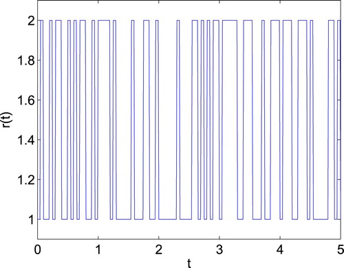
Furthermore, the homogeneous Markovian chain $\sigma \left(t\right)$ takes value in $\mathcal{V}=\{1,2,3\}$, and the corresponding TR matrix with partly unknown information is taken as $\mathrm{\Pi }=\left[\begin{array}{ccc}-1.0& ?& ?\\ ?& -0.9& ?\\ ?& ?& -1.2\end{array}\right].$ The piecewise-homogeneous TR matrix of Markovian chain $r\left(t\right)$ are taken as follows: $\begin{array}{rl}& {\mathrm{\Lambda }}^1=\left[\begin{array}{cc}-0.8& 0.8\\ 0.9& -0.9\end{array}\right],{\mathrm{\Lambda }}^2=\left[\begin{array}{cc}-0.8& 0.8\\ 0.6& -0.6\end{array}\right],\\ & {\mathrm{\Lambda }}^3=\left[\begin{array}{cc}-0.7& 0.7\\ 1.0& -1.0\end{array}\right].\end{array}$ Therefore, we can easily obtain that $\overline{\lambda }=1.0$, $\overline{\pi }=1.2$. For the purpose of simulation, the homogeneous Markovian process $\sigma \left(t\right)$ is shown in Figure 2, and the piecewise-homogeneous Markovian process $r\left(t\right)$ is shown in Figure 3.

Figure 2. Variation of the homogeneous Markovian process $\sigma \left(t\right)$ with three modes.

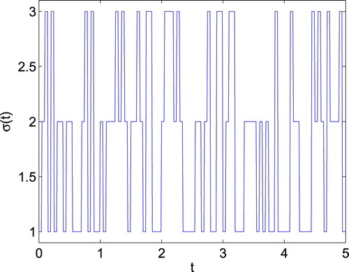
Figure 3. Variation of the piecewise-homogeneous Markovian process $r\left(t\right)$ with two modes.

The mode-dependent time-varying delays are set as ${\tau }_{1,1}\left(t\right)=0.6+0.02\sin \left(4t\right)$, ${\tau }_{1,2}\left(t\right)=0.4+0.06\sin \left(2t\right)$, ${\tau }_{1,3}\left(t\right)=0.8+0.05\sin \left(10t\right)$, ${\tau }_{2,1}\left(t\right)=0.7+0.04\cos \left(3t\right)$, ${\tau }_{2,2}\left(t\right)=0.2+0.04\cos \left(3t\right)$, ${\tau }_{2,3}\left(t\right)=0.6+0.05\cos \left(4t\right)$. It can be derived that ${\tau }_1=0.16$, ${\tau }_2=0.85$ and $\overline{\tau }=0.5$.

Take the constant $\text{β}=0.3$, by resorting to Theorem 3.1, it can be calculated that inequalities (9(9) $\begin{array}{rl}& {\mathrm{\Gamma }}_{\iota }\le G_{\iota },\end{array}$(9) )–(12(12) $\begin{array}{rl}& \left\{\begin{array}{ll}{P}_{i,n}-T_{i,m}\le 0,& n\in {\mathcal{V}}_{uk}^m\mathrm{\setminus }\left\{m\right\}\\ P_{i,n}-T_{i,m}\ge 0,& n\in {\mathcal{V}}_{uk}^m\cap \left\{m\right\}\end{array}\right.\end{array}$(12) ) have feasible solutions as $\begin{array}{rl}{P}_{1,1}& =\left[\begin{array}{cccc}0.6927& 0.0295& 0& 0\\ 0.0295& 0.8462& 0& 0\\ 0& 0& 0.6832& 0.0432\\ 0& 0& 0.0432& 0.8372\end{array}\right],\\ P_{2,3}& =\left[\begin{array}{cccc}0.7456& 0.0275& 0& 0\\ 0.0275& 0.7623& 0& 0\\ 0& 0& 0.7372& 0.0443\\ 0& 0& 0.0443& 0.7568\end{array}\right],\\ G_1& =\mathrm{d}\mathrm{i}\mathrm{a}\mathrm{g}\{0.1228,0.1360,0.1144,0.1362\},{\vartheta }_{\iota }=1\end{array}$ and the other matrices are omitted for space consideration. Therefore, it follows from Theorem 3.1 that system (6(6) $\begin{array}{rl}\dot{\xi }\left(t\right)& =-C_{1i}\xi \left(t\right)+A_{1i}{f}_1\left(\xi \right(t\left)\right)+A_{2i}{f}_2\left(\xi \right(t\left)\right)+u\left(t\right)\\ & +B_{1i}{g}_1\left(\xi \right(t-{\tau }_{i,m}\left(t\right)\left)\right)+B_{2i}{g}_2\left(\xi \right(t-{\tau }_{i,m}\left(t\right)\left)\right)\end{array}$(6) ) with $u\left(t\right)\equiv 0$ is exponentially stable in the mean-square sense.

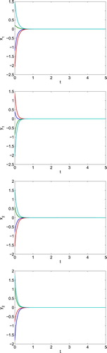
For simulation aim, the following four cases of initial conditions are taken. Case 1: $z_1\left(t\right)=-1.2+0.4\overrightarrow{\mathrm{i}}$, $z_2\left(t\right)=0.2-0.9\overrightarrow{\mathrm{i}}$ for $t\in [-0.85,0]$. Case 2: $z_1\left(t\right)=-2.1+1.4\overrightarrow{\mathrm{i}}$, $z_2\left(t\right)=1.5-2.1\overrightarrow{\mathrm{i}}$ for $t\in [-0.85,0]$. Case 3: $z_1\left(t\right)=-0.8-1.8\overrightarrow{\mathrm{i}}$, $z_2\left(t\right)=0.6+1.1\overrightarrow{\mathrm{i}}$ for $t\in [-0.85,0]$. Case 4: $z_1\left(t\right)=1.6-0.8\overrightarrow{\mathrm{i}}$, $z_2\left(t\right)=1.6+1.8\overrightarrow{\mathrm{i}}$ for $t\in [-0.85,0]$. When $\tilde{u}\left(t\right)\equiv 0$, the time responses of the real and imaginary parts of state $z\left(t\right)$ are shown in Figure 4, which further demonstrates that the piecewise-homogeneous Markovian switching CVNN (1(1) $\begin{array}{rl}\dot{z}\left(t\right)& =-C\left(r\right(t\left)\right)z\left(t\right)+A\left(r\right(t\left)\right)f\left(z\right(t\left)\right)\\ & +B\left(r\right(t\left)\right)g\left(z\right(t-{\tau }_{r\left(t\right),\sigma \left(t\right)}\left(t\right)\left)\right)+\tilde{u}\left(t\right),t\ge 0\end{array}$(1) ) with parameters above is 0.6-exponentially stable in the mean-square sense.

Figure 4. Time responses of the real/imaginary parts of state $z\left(t\right)$ for CVNN (1(1) $\begin{array}{rl}\dot{z}\left(t\right)& =-C\left(r\right(t\left)\right)z\left(t\right)+A\left(r\right(t\left)\right)f\left(z\right(t\left)\right)\\ & +B\left(r\right(t\left)\right)g\left(z\right(t-{\tau }_{r\left(t\right),\sigma \left(t\right)}\left(t\right)\left)\right)+\tilde{u}\left(t\right),t\ge 0\end{array}$(1) ) with $\tilde{u}\left(t\right)\equiv 0$ in Example 4.1.

Example 4.2

Consider the piecewise-homogeneous Markovian switching CVNN (1(1) $\begin{array}{rl}\dot{z}\left(t\right)& =-C\left(r\right(t\left)\right)z\left(t\right)+A\left(r\right(t\left)\right)f\left(z\right(t\left)\right)\\ & +B\left(r\right(t\left)\right)g\left(z\right(t-{\tau }_{r\left(t\right),\sigma \left(t\right)}\left(t\right)\left)\right)+\tilde{u}\left(t\right),t\ge 0\end{array}$(1) ) with $C_1=\mathrm{d}\mathrm{i}\mathrm{a}\mathrm{g}\{1.9,2.1\}$, $C_2=\mathrm{d}\mathrm{i}\mathrm{a}\mathrm{g}\{1.8,2.0\}$, and $\begin{array}{rl}& A_1=\left[\begin{array}{cc}1.0-1.2\overrightarrow{\mathrm{i}}& 0.8+0.9\overrightarrow{\mathrm{i}}\\ 1.6+1.2\overrightarrow{\mathrm{i}}& 1.4+1.5\overrightarrow{\mathrm{i}}\end{array}\right],\\ & B_1=\left[\begin{array}{cc}0.8+1.0\overrightarrow{\mathrm{i}}& 0.9+0.8\overrightarrow{\mathrm{i}}\\ 1.2+1.8\overrightarrow{\mathrm{i}}& 1.6-1.0\overrightarrow{\mathrm{i}}\end{array}\right],\\ & A_2=\left[\begin{array}{cc}1.8+1.4\overrightarrow{\mathrm{i}}& 1.4+1.0\overrightarrow{\mathrm{i}}\\ 1.3-0.8\overrightarrow{\mathrm{i}}& 0.6+1.2\overrightarrow{\mathrm{i}}\end{array}\right],\\ & B_2=\left[\begin{array}{cc}0.9+0.8\overrightarrow{\mathrm{i}}& 0.7+1.2\overrightarrow{\mathrm{i}}\\ 0.9-0.6\overrightarrow{\mathrm{i}}& 1.4+1.1\overrightarrow{\mathrm{i}}\end{array}\right].\end{array}$ In addition, the piecewise-homogeneous Markovian process $r\left(t\right)$, the homogeneous Markovian process $\sigma \left(t\right)$, the activation functions $f_{\upsilon }\left(z_{\upsilon }\right)$ and $g_{\upsilon }\left(z_{\upsilon }\right)$, and the mode-dependent time-varying delay ${\tau }_{r\left(t\right),\sigma \left(t\right)}\left(t\right)$ are the same as taken in Example 4.1.

Solving the inequalities (9(9) $\begin{array}{rl}& {\mathrm{\Gamma }}_{\iota }\le G_{\iota },\end{array}$(9) )–(12(12) $\begin{array}{rl}& \left\{\begin{array}{ll}{P}_{i,n}-T_{i,m}\le 0,& n\in {\mathcal{V}}_{uk}^m\mathrm{\setminus }\left\{m\right\}\\ P_{i,n}-T_{i,m}\ge 0,& n\in {\mathcal{V}}_{uk}^m\cap \left\{m\right\}\end{array}\right.\end{array}$(12) ), and (28(28) $\begin{array}{rl}& \left[\begin{array}{cccccc}{\tilde{\mathrm{\Xi }}}_{11}& 0& 0& 0& P_{i,m}{A}_{1i}& P_{i,m}{A}_{2i}\\ \ast & {\mathrm{\Xi }}_{22}& {\mathrm{\Xi }}_{23}& S& 0& 0\\ \ast & \ast & {\mathrm{\Xi }}_{33}& {\mathrm{\Xi }}_{34}& 0& 0\\ \ast & \ast & \ast & {\mathrm{\Xi }}_{44}& 0& 0\\ \ast & \ast & \ast & \ast & {\mathrm{\Xi }}_{55}& 0\\ \ast & \ast & \ast & \ast & \ast & {\mathrm{\Xi }}_{66}\\ \ast & \ast & \ast & \ast & \ast & \ast \\ \ast & \ast & \ast & \ast & \ast & \ast \\ \ast & \ast & \ast & \ast & \ast & \ast \end{array}\right.\\ & \left.\begin{array}{ccc}{P}_{i,m}{B}_{1i}& P_{i,m}{B}_{2i}& {\tilde{\mathrm{\Xi }}}_{19}\\ 0& 0& 0\\ 0& 0& 0\\ 0& 0& 0\\ 0& 0& ({\tau }_2-{\tau }_1)A_{1i}^{\mathrm{T}}{P}_{i,m}\\ 0& 0& ({\tau }_2-{\tau }_1)A_{2i}^{\mathrm{T}}{P}_{i,m}\\ {\mathrm{\Xi }}_{77}& 0& ({\tau }_2-{\tau }_1)B_{1i}^{\mathrm{T}}{P}_{i,m}\\ \ast & {\mathrm{\Xi }}_{88}& ({\tau }_2-{\tau }_1)B_{2i}^{\mathrm{T}}{P}_{i,m}\\ \ast & \ast & R-2P_{i,m}\end{array}\right]<0\end{array}$(28) ) with $\text{β}=0.2$, it is easy to obtain the following feasible solutions ${\vartheta }_{\iota }=10$, and $\begin{array}{rl}{P}_{1,1}& =\left[\begin{array}{cccc}10.7302& -2.2293& 0& 0\\ -2.2293& 9.5265& 0& 0\\ 0& 0& 16.2529& -9.3086\\ 0& 0& -9.3086& 14.2854\end{array}\right],\\ Y_{1,1}& =\left[\begin{array}{cccc}-5.5474& -3.9855& 0& 0\\ -2.8861& -8.4901& 0& 0\\ 0& 0& 0.0459& -9.2115\\ 0& 0& -6.7680& 2.0681\end{array}\right]\end{array}$ and the other matrices are omitted for space consideration. The gain matrices of the state feedback controller are designed as $\begin{array}{rl}{K}_{1,1}& =\left[\begin{array}{cccc}-0.6096& -0.5850& 0& 0\\ -0.4456& -1.0281& 0& 0\\ 0& 0& -0.4284& -0.7719\\ 0& 0& -0.7529& -0.3582\end{array}\right],\\ K_{1,2}& =\left[\begin{array}{cccc}-0.5609& -0.6426& 0& 0\\ -0.5070& -1.1558& 0& 0\\ 0& 0& -0.3401& -0.9047\\ 0& 0& -0.7369& -0.5247\end{array}\right],\\ K_{1,3}& =\left[\begin{array}{cccc}-0.6996& -0.4552& 0& 0\\ -0.3260& -1.0547& 0& 0\\ 0& 0& -0.6102& -0.5287\\ 0& 0& -0.8068& -0.2215\end{array}\right],\\ K_{2,1}& =\left[\begin{array}{cccc}0.4036& -0.9375& 0& 0\\ -0.5993& -0.6736& 0& 0\\ 0& 0& 0.5991& -1.3714\\ 0& 0& 0.0268& -0.7130\end{array}\right],\\ K_{2,2}& =\left[\begin{array}{cccc}-0.6880& -0.5920& 0& 0\\ -0.4536& -1.1445& 0& 0\\ 0& 0& -0.5063& -0.8101\\ 0& 0& -0.7002& -0.5411\end{array}\right],\\ K_{2,3}& =\left[\begin{array}{cccc}-0.7332& -0.6120& 0& 0\\ -0.4699& -1.1987& 0& 0\\ 0& 0& -0.5364& -0.8173\\ 0& 0& -0.7656& -0.5199\end{array}\right].\end{array}$ It follows from Theorem 3.2 that the CVNN (1(1) $\begin{array}{rl}\dot{z}\left(t\right)& =-C\left(r\right(t\left)\right)z\left(t\right)+A\left(r\right(t\left)\right)f\left(z\right(t\left)\right)\\ & +B\left(r\right(t\left)\right)g\left(z\right(t-{\tau }_{r\left(t\right),\sigma \left(t\right)}\left(t\right)\left)\right)+\tilde{u}\left(t\right),t\ge 0\end{array}$(1) ) with system parameters as above is 0.4-exponentially stabilizable in the mean-square sense.

In the following, we give the corresponding numerical simulations. Four cases of initial conditions are taken. Case 1: $z_1\left(t\right)=-1.4+0.3\overrightarrow{\mathrm{i}}$, $z_2\left(t\right)=0.4-0.3\overrightarrow{\mathrm{i}}$ for $t\in [-0.85,0]$. Case 2: $z_1\left(t\right)=-1.7+1.3\overrightarrow{\mathrm{i}}$, $z_2\left(t\right)=1.4-1.7\overrightarrow{\mathrm{i}}$ for $t\in [-0.85,0]$. Case 3: $z_1\left(t\right)=-0.2-1.5\overrightarrow{\mathrm{i}}$, $z_2\left(t\right)=0.9+1.3\overrightarrow{\mathrm{i}}$ for $t\in [-0.85,0]$. Case 4: $z_1\left(t\right)=-1.2-0.6\overrightarrow{\mathrm{i}}$, $z_2\left(t\right)=1.3+1.4\overrightarrow{\mathrm{i}}$ for $t\in [-0.85,0]$. When $\tilde{u}\left(t\right)\equiv 0$, the time responses of the real and imaginary parts of state $z\left(t\right)$ for the open-loop system (1(1) $\begin{array}{rl}\dot{z}\left(t\right)& =-C\left(r\right(t\left)\right)z\left(t\right)+A\left(r\right(t\left)\right)f\left(z\right(t\left)\right)\\ & +B\left(r\right(t\left)\right)g\left(z\right(t-{\tau }_{r\left(t\right),\sigma \left(t\right)}\left(t\right)\left)\right)+\tilde{u}\left(t\right),t\ge 0\end{array}$(1) ) with mode-dependent time-varying delays and partly unknown TRs are shown in Figure 5. It is obvious that the open-loop system (1(1) $\begin{array}{rl}\dot{z}\left(t\right)& =-C\left(r\right(t\left)\right)z\left(t\right)+A\left(r\right(t\left)\right)f\left(z\right(t\left)\right)\\ & +B\left(r\right(t\left)\right)g\left(z\right(t-{\tau }_{r\left(t\right),\sigma \left(t\right)}\left(t\right)\left)\right)+\tilde{u}\left(t\right),t\ge 0\end{array}$(1) ) is unstable. Figure 6 illustrates the corresponding ones for the closed-loop system (1(1) $\begin{array}{rl}\dot{z}\left(t\right)& =-C\left(r\right(t\left)\right)z\left(t\right)+A\left(r\right(t\left)\right)f\left(z\right(t\left)\right)\\ & +B\left(r\right(t\left)\right)g\left(z\right(t-{\tau }_{r\left(t\right),\sigma \left(t\right)}\left(t\right)\left)\right)+\tilde{u}\left(t\right),t\ge 0\end{array}$(1) ) with mode-dependent controller (26(26) $u\left(t\right)=K_{r\left(t\right),\sigma \left(t\right)}\xi \left(t\right).$(26) ), which further confirm the effectiveness of the proposed control scheme.

Figure 5. Time responses of the real/imaginary parts of state $z\left(t\right)$ for the open-loop system (1(1) $\begin{array}{rl}\dot{z}\left(t\right)& =-C\left(r\right(t\left)\right)z\left(t\right)+A\left(r\right(t\left)\right)f\left(z\right(t\left)\right)\\ & +B\left(r\right(t\left)\right)g\left(z\right(t-{\tau }_{r\left(t\right),\sigma \left(t\right)}\left(t\right)\left)\right)+\tilde{u}\left(t\right),t\ge 0\end{array}$(1) ) in Example 4.2.

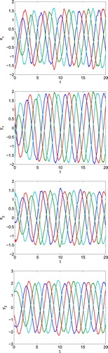
Figure 6. Time responses of the real/imaginary parts of state $z\left(t\right)$ for the closed-loop system (1(1) $\begin{array}{rl}\dot{z}\left(t\right)& =-C\left(r\right(t\left)\right)z\left(t\right)+A\left(r\right(t\left)\right)f\left(z\right(t\left)\right)\\ & +B\left(r\right(t\left)\right)g\left(z\right(t-{\tau }_{r\left(t\right),\sigma \left(t\right)}\left(t\right)\left)\right)+\tilde{u}\left(t\right),t\ge 0\end{array}$(1) ) in Example 4.2.

5. Conclusion

In this paper, the stability and stabilization problems have been investigated for a class of piecewise-homogeneous Markovian switching CVNNs with mode-dependent time-varying delays and partly known TRs. The TRs of the piecewise-homogeneous Markov process are time-varying in different intervals but invariant during one interval. Moreover, the TR information of the two-level Markov processes is partially known, and the time-varying delays are mode-dependent. By utilizing the Lyapunov theory, sufficient conditions have been established to ensure the considered system to be exponentially stable (stabilizable) in the mean-square sense. Finally, two numerical examples are provided to illustrate the effectiveness of the proposed results.

In the future, further investigations will be carried out for the stabilization/estimation problems of semi-Markovian switching CVNNs with mode-dependent time-varying delays, where the sojourn-time obeys the non-exponential distribution and the TR information is incomplete, which might better characterize certain practical systems.

Disclosure statement

No potential conflict of interest was reported by the author(s).

Additional information

Funding

This work was supported by the National Natural Science Foundation of China [Grant Number 61673110 and 61906084], the Natural Science Foundation of Jiangsu Province of China [Grant Number BK20180815], and The Scientific Research Foundation of Graduate School of Southeast University [Grant Number YBPY1870].

References

- Anderson, R. J., & Spong, M. W. (1989). Bilateral control of teleoperators with time delay. IEEE Transactions on Automatic Control, 34(5), 494–501. https://doi.org/10.1109/9.24201
- Boyd, S., El Ghaoui, L., Feron, E., & Balakrishnan, V. (1994). Linear matrix inequalities in system and control theory. SIAM.
- Cui, K., Zhu, J., & Li, C. (2019). Exponential stabilization of Markov jump systems with mode-dependent mixed time-varying delays and unknown transition rates. Circuits, Systems, and Signal Processing, 38(10), 4526–4547. https://doi.org/10.1007/s00034-019-01085-2
- Du, B., Lam, J., Zou, Y., & Shu, Z. (2013). Stability and stabilization for Markovian jump time-delay systems with partially unknown transition rates. IEEE Transactions on Circuits and Systems I: Regular Papers, 60(2), 341–351. https://doi.org/10.1109/TCSI.2012.2215791
- Dynkin, E. B. (1965). Markov processes. Springer.
- Goh, S. L., & Mandic, D. P. (2004). A complex-valued RTRL algorithm for recurrent neural networks. Neural Computation, 16(12), 2699–2713. https://doi.org/10.1162/0899766042321779
- Goh, S. L., & Mandic, D. P. (2007). An augmented extended Kalman filter algorithm for complex-valued recurrent neural networks. Neural Computation, 19(4), 1039–1055. https://doi.org/10.1162/neco.2007.19.4.1039
- Gong, W., Liang, J., & Cao, J. (2015). Matrix measure method for global exponential stability of complex-valued recurrent neural networks with time-varying delays. Neural Networks, 70, 81–89. https://doi.org/10.1016/j.neunet.2015.07.003
- Guo, Y. (2016). Necessary and sufficient conditions for analysis and synthesis of Markov jump systems with partially known transition rates. Journal of the Franklin Institute, 353(8), 1920–1930. https://doi.org/10.1016/j.jfranklin.2016.02.021
- Hirose, A. (1992a). Continuous complex-valued back-propagation learning. Electronics Letters, 28(20), 1854–1855. https://doi.org/10.1049/el:19921186
- Hirose, A. (1992b). Dynamics of fully complex-valued neural networks. Electronics Letters, 28(16), 1492–1494. https://doi.org/10.1049/el:19920948
- Jankowski, S., Lozowski, A., & Zurada, J. M. (1996). Complex-valued multistate neural associative memory. IEEE Transactions on Neural Networks, 7(6), 1491–1496. https://doi.org/10.1109/72.548176
- Kobayashi, M. (2018). Singularities of three-layered complex-valued neural networks with split activation function. IEEE Transactions on Neural Networks and Learning Systems, 29(5), 1900–1907. https://doi.org/10.1109/TNNLS.2017.2688322
- Li, Q., Liang, J., & Gong, W. (2019). Stability and synchronization for impulsive Markovian switching CVNNs: Matrix measure approach. Communications in Nonlinear Science and Numerical Simulation, 77, 126–140. https://doi.org/10.1016/j.cnsns.2019.04.022
- Liang, J., Gong, W., & Huang, T. (2016). Multistability of complex-valued neural networks with discontinuous activation functions. Neural Networks, 84, 125–142. https://doi.org/10.1016/j.neunet.2016.08.008
- Liu, X., & Chen, T. (2015). Global exponential stability for complex-valued recurrent neural networks with asynchronous time delays. IEEE Transactions on Neural Networks and Learning Systems, 27(3), 593–606. https://doi.org/10.1109/TNNLS.5962385 doi: 10.1109/TNNLS.2015.2415496
- Liu, Z.-X., Park, J. H., & Wu, Z.-G. (2013). Synchronization of complex networks with nonhomogeneous Markov jump topology. Nonlinear Dynamics, 74(1–2), 65–75. https://doi.org/10.1007/s11071-013-0949-x
- Liu, L., Wang, Y., Ma, L., Zhang, J., & Bo, Y. (2018). Robust finite-horizon filtering for nonlinear time-delay Markovian jump systems with weighted try-once-discard protocol. Systems Science & Control Engineering: An Open Access Journal, 6(1), 180–194. https://doi.org/10.1080/21642583.2018.1474396
- Luo, Y., Wang, Z., Liang, J., Wei, G., & Alsaadi, F. E. (2017). H∞ control for 2-D fuzzy systems with interval time-varying delays and missing measurements. IEEE Transactions on Cybernetics, 47(2), 365–377. https://doi.org/10.1109/TCYB.2016.2514846
- Luo, Y., Wang, Z., Wei, G., & Alsaadi, F. E. (2020). Nonfragile l2-l∞ fault estimation for Markovian jump 2-D systems with specified power bounds. IEEE Transactions on Systems, Man, and Cybernetics: Systems. https://doi.org/10.1109/TSMC.2018.2794414
- Ma, L., Wang, L., Han, Q.-L., & Liu, Y. (2018). Dissipative control for nonlinear Markovian jump systems with actuator failures and mixed time-delays. Automatica, 98, 358–362. https://doi.org/10.1016/j.automatica.2018.09.028
- Nagamani, G., Radhika, T., & Gopalakrishnan, P. (2017). Dissipativity and passivity analysis of Markovian jump impulsive neural networks with time delays. International Journal of Computer Mathematics, 94(7), 1479–1500. https://doi.org/10.1080/00207160.2016.1190013
- Park, P. G., Ko, J. W., & Jeong, C. (2011). Reciprocally convex approach to stability of systems with time-varying delays. Automatica, 47(1), 235–238. https://doi.org/10.1016/j.automatica.2010.10.014
- Samidurai, R., Sriraman, R., & Zhu, S. (2019). Leakage delay-dependent stability analysis for complex-valued neural networks with discrete and distributed time-varying delays. Neurocomputing, 338, 262–273. https://doi.org/10.1016/j.neucom.2019.02.027
- Shen, H., Zhu, Y., Zhang, L., & Park, J. H. (2016). Extended dissipative state estimation for Markov jump neural networks with unreliable links. IEEE Transactions on Neural Networks and Learning Systems, 28(2), 346–358. https://doi.org/10.1109/TNNLS.2015.2511196
- Song, M. K., Park, J. B., & Joo, Y. H. (2014). Stability analysis and fuzzy control for Markovian jump nonlinear systems with partially unknown transition probabilities. IEICE Transactions on Fundamentals of Electronics, Communications and Computer Sciences, 97(2), 587–596. https://doi.org/10.1587/transfun.E97.A.587
- Song, Q., & Zhao, Z. (2016). Stability criterion of complex-valued neural networks with both leakage delay and time-varying delays on time scales. Neurocomputing, 171, 179–184. https://doi.org/10.1016/j.neucom.2015.06.032
- Wang, H., Duan, S., Huang, T., Wang, L., & Li, C. (2016). Exponential stability of complex-valued memristive recurrent neural networks. IEEE Transactions on Neural Networks and Learning Systems, 28(3), 766–771. https://doi.org/10.1109/TNNLS.2015.2513001
- Wang, L., Wang, Z., Wei, G., & Alsaadi, F. E. (2018). Finite-time state estimation for recurrent delayed neural networks with component-based event-triggering protocol. IEEE Transactions on Neural Networks and Learning Systems, 29(4), 1046–1057. https://doi.org/10.1109/TNNLS.2016.2635080
- Wang, P., Zou, W., & Su, H. (2019). Stability of complex-valued impulsive stochastic functional differential equations on networks with Markovian switching. Applied Mathematics and Computation, 348, 338–354. https://doi.org/10.1016/j.amc.2018.12.006
- Wu, Z.-G., Park, J. H., Su, H., & Chu, J. (2012a). Passivity analysis of Markov jump neural networks with mixed time-delays and piecewise-constant transition rates. Nonlinear Analysis: Real World Applications, 13(5), 2423–2431. https://doi.org/10.1016/j.nonrwa.2012.02.009
- Wu, Z.-G., Park, J. H., Su, H., & Chu, J. (2012b). Stochastic stability analysis of piecewise homogeneous Markovian jump neural networks with mixed time-delays. Journal of the Franklin Institute, 349(6), 2136–2150. https://doi.org/10.1016/j.jfranklin.2012.03.005
- Yang, Z., & Liao, X. (2019). Invariant and attracting sets of complex-valued neural networks with both time-varying and infinite distributed delays. Neural Processing Letters, 49(3), 1201–1215. https://doi.org/10.1007/s11063-018-9848-y
- Yang, X., Song, Q., Cao, J., & Lu, J. (2018). Synchronization of coupled Markovian reaction-diffusion neural networks with proportional delays via quantized control. IEEE Transactions on Neural Networks and Learning Systems, 30(3), 951–958. https://doi.org/10.1109/TNNLS.2018.2853650
- Zhang, L. (2009). H∞ estimation for discrete-time piecewise homogeneous Markov jump linear systems. Automatica, 45(11), 2570–2576. https://doi.org/10.1016/j.automatica.2009.07.004
- Zhang, L., & Boukas, E. K. (2009). H∞ control for discrete-time Markovian jump linear systems with partly unknown transition probabilities. International Journal of Robust and Nonlinear Control, 19(8), 868–883. https://doi.org/10.1002/rnc.v19:8 doi: 10.1002/rnc.1355
- Zhang, X., Chen, L., & Chen, Y. (2019). Consensus analysis of multi-agent systems with general linear dynamics and switching topologies by non-monotonically decreasing Lyapunov function. Systems Science & Control Engineering: An Open Access Journal, 7(1), 179–188. https://doi.org/10.1080/21642583.2019.1620654
- Zhang, T., Gao, J., & Li, J. (2018). Event-triggered H∞ filtering for discrete-time Markov jump delayed neural networks with quantizations. Systems Science & Control Engineering: An Open Access Journal, 6(3), 74–84. https://doi.org/10.1080/21642583.2018.1531360
- Zhang, L., & Lam, J. (2010). Necessary and sufficient conditions for analysis and synthesis of Markov jump linear systems with incomplete transition descriptions. IEEE Transactions on Automatic Control, 55(7), 1695–1701. https://doi.org/10.1109/TAC.2010.2046607
- Zhang, C., Wang, X., Wang, S., Zhou, W., & Xia, Z. (2018). Finite-time synchronization for a class of fully complex-valued networks with coupling delay. IEEE Access, 6, 17923–17932. https://doi.org/10.1109/ACCESS.2018.2818192
- Zhang, L., Zhu, Y., Shi, P., & Zhao, Y. (2015). Resilient asynchronous H∞ filtering for Markov jump neural networks with unideal measurements and multiplicative noises. IEEE Transactions on Cybernetics, 45(12), 2840–2852. https://doi.org/10.1109/TCYB.2014.2387203