Tooth identification based on teeth structure feature

Abstract

Massive disasters, like earthquake and fire, can easily damage most features of the human body, which bring difficulties in cadaver identification. In this paper, to improve the efficiency and accuracy of forensic autopsy, a novel tooth identification strategy based on teeth structure features from dental impression images is proposed. The strategy achieves identification including tooth mark segmentation, teeth structure feature extraction, and matching. To resolve the problem of too much noise, we propose a locating segmentation method based on object detection to segment every single tooth mark contour. Finally, to evaluate the proposed strategy more objectively, we propose an indicator named rate of filtration based on the indicator accuracy. The experimental results show that using only upper-jaw teeth, our method achieves a rate of filtration of 90.45% for 47 persons comprised of 311 images, and an accuracy of 86.17% for top-5 (top 12%) image matching, which are highly encouraging. To the best of our knowledge, the proposed method is the first to use dental impression images to achieve tooth identification.

KEYWORDS:

• Tooth identification
• forensic identification
• tooth feature
• image processing

1. Introduction

Biometric identification has always been important in many domains. In law enforcement sector, ‘forensic identification may take place prior to death, which is referred to as Antemortem (AM) identification while may also be carried out after death and this is called Postmortem (PM) identification’ (Fahmy & Nassar, 2004). In general, biometrics mainly focus on human face, fingerprint, iris, palm print and so on. These methods require features without severe deformation, which are more suitable for AM identification. However, in some situations, like natural disasters (earthquakes, floods, fires, etc.) and crime scenes, human faces and other superficial features may be highly damaged, which makes most of them not suitable for PM identification. Meanwhile, although DNA is accurate, it is expensive, time-consuming and hard to be applied in a large number of PM identification in emergencies. Therefore, as the most indestructible part of human body, teeth, whose enamel on the surface has strong high-temperature and corrosion resistance, can not only replace the features like human faces, improving the accuracy of autopsy, but also greatly reduce the range of candidates, assisting or even replacing DNA methods and improving the efficiency, which makes them the best choice for PM identification (Lin et al., 2010).

In the past decades, there have been some tooth identification methods available in existing literatures. Most of them use dental radiograph as original images. For example, an Automatic Dental Identification System (ADIS) has been proposed in Zhou and Abdel-Mottaleb (2005), Nomir and Abdel-Mottaleb (2005), Nomir and Abdel-Mottaleb (2008a). Then some methods using tooth contours as matching features are proposed in Jain and Chen (2004), Nomir and Abdel-Mottaleb (2008b). In addition, features of dental works (DWs) such as crowns, bridges and dental fillings are found significant. Chen and Jain (2005) proposed to use an area-based metric fusing both tooth contours and DWs. Hofer and Marana (2007) proposed a tooth identification method based on DWs, including the position, size and distance between adjacent DWs. Furthermore, a feature vector including prominent points of the tooth contours with high curvature has been proposed in Nomir and Abdel-Mottaleb (2007). And additional invariant frequency features are highlighted when matching with spatial features of DWs in Lin et al. (2012). Otherwise, different with contour features, Rajput and Mahajan (2016) proposed a method based on the overall skeleton of teeth and Banday and Mir (2019) proposed a novel mandibular biometric identification system that builds an AR model of individual teeth. For contour features in Zhou and Abdel-Mottaleb (2005), Nomir and Abdel-Mottaleb (2005), Nomir and Abdel-Mottaleb (2008a), Jain and Chen (2004), Nomir and Abdel-Mottaleb (2008b), Chen and Jain (2005), Hofer and Marana (2007), Nomir and Abdel-Mottaleb (2007), Lin et al. (2012), different shooting angles may deform shapes of contours and lead to mismatch. For global features in Rajput and Mahajan (2016), Banday and Mir (2019), they are short on details. Therefore, in this paper, we obtain contours of tooth marks first and further compute multiple global teeth structure features based on contour features, which combining both overall and details.

Recently, according to the survey (Minaee et al., 2019), some biometric models based on deep learning have achieved considerably good result. And for tooth identification, a ToothNet using learned edge maps, similarity matrices, and spatial relationships between teeth has been first proposed in Cui et al. (2019).

Above-mentioned methods all use dental radiographs, while radiation is harmful to human body. Thus, people are only willing to take a dental radiograph when their teeth are sick, making it difficult to collect multiple X-rays of healthy people and not support to a large-scale training. Therefore, some radiation-free methods using colour images of the front of teeth have been proposed in Rehman et al. (2015) and Kumar (2016). They processed the grayscales, extracted high-intensity areas and compare the overall similarity. However, this kind of images only contains the external information of frontal teeth, which may not accurate enough. Different with existing radiation-free methods, the proposed method in this paper is aimed at internal information of teeth, segmenting tooth contours, calculating structure features and matching, which is more comprehensive. To the best of our knowledge, our strategy is the first to use images of dental impression models for identification.

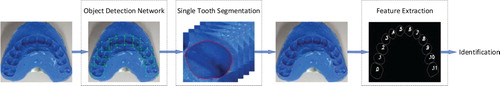
In response to the above discussions, the main contributions of this paper are summarized as follows: (1) Proposed a novel dental biometric strategy based on teeth structural features using dental impression images shown in Figure 1(a). Figure 2 shows the flowchart of the entire algorithm; (2) Propose a locating segmentation method based on object detection for tooth contours. We detect every single tooth mark as an object using the object detection network to obtain the boundary box, so that the region of interest (ROI) is divided for segmentation; (3) A novel indicator named rate of filtration (ROF) is proposed. In order to evaluate the biometric algorithm more comprehensively and objectively, the indicator rate of filtration is proposed instead of accuracy.

Figure 1. (a) A dental impression model image. (b) The contoured dental impression image. (c) Training data of object detection. (d) One test result of object detection.

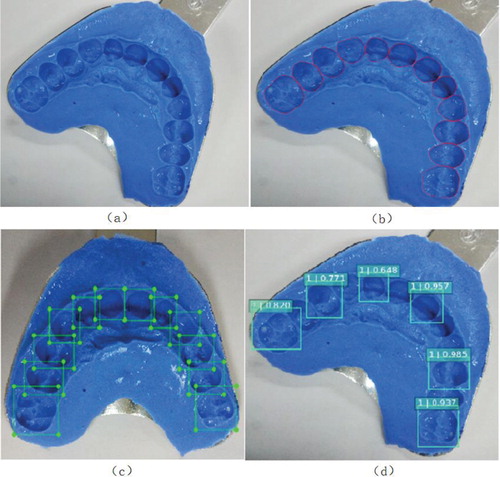
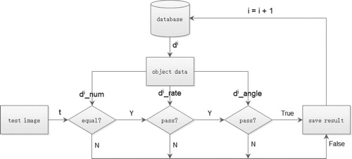
Figure 2. Our processing flow of the proposed strategy. Given a dental impression image, we first detect every tooth mark and obtain their bounding boxes. Then the bounding boxes are set as regions of interest for segmentation of every single tooth mark. Finally, geometric features are extracted from the contoured image and used to identify.

The rest of this paper is organized as follows. Section 2 elaborates the proposed segmentation method and Section 3 supplements the additional contour extraction for some hard-segmenting images. Section 4 elaborates feature extraction and classification. Experimental results and comparison are reported in Section 5. Finally, we conclude the paper in Section 6.

2. Contour segmentation

Image segmentation has always been a basic step in image processing. Most visual tasks need to obtain the area, position or contour of the object in the image for subsequent work. Classic segmentation algorithms generally include threshold segmentation, watershed algorithm (Gonzalez & Woods, 2010), etc. However, a simple threshold usually cannot segment well for complex images and watershed algorithms have to mark seeds, which is not very automatic. Recently, there have also been some methods based on neural networks (Badrinarayanan et al., 2017; Lin et al., 2017; Long et al., 2015), often used for daily scenes such as street. Moreover, Chen et al. (2017) proposed a system named DeepLab that re-purposes the neural networks which have been trained on image classification to semantic segmentation and significantly improve the effect. Jader et al. (2018) proposed a segmentation system based on mask region-based convolutional neural network to complete the detection and segmentation of each tooth in the panoramic X-ray image.

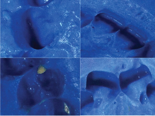
However, due to the complex texture, blurry and unrecognizable contours, and potholes shown in Figure 3, general methods cannot segment well for dental impression images. This paper proposes a feasible tooth contour segmentation scheme. We use an object detection network named single shot multibox detector (SSD) (Liu et al., 2016) to locate contours and define a series of bounding boxes, and then segment tooth marks one by one, which greatly reduces the interference from non-tooth contours. To solve problems of unclear contour edges, we extract rough edges with Sobel operator (Gonzalez & Woods, 2010), filter, pair and fit edge fragments to obtain a single tooth contour.

Figure 3. Problems in segmentation.

2.1. Object detection

Object detection has made important progress in recent years. Algorithms are mainly divided into two types: One-stage method and two-stage method. The one-stage samples with different scales and aspect ratios, and perform classification and regression directly. While the two-stage generates a series of sparse candidate boxes first by selective search method (Uijlings et al., 2013) or convolutional neural network (CNN) (Krizhevsky et al., 2012), and then perform classification and regression, with high accuracy but low speed.

SSD (Liu et al., 2016), one of the one-stage methods, can be divided into three steps:

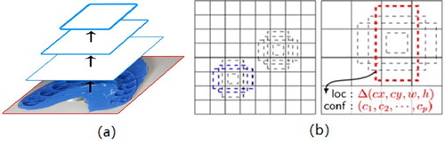
1. Pre-process images and extract multi-scale high-dimensional feature maps by CNN, as shown in Figure 4(a). CNN obtains the first feature map by convolving the original image, and re-convolves it to obtain a higher-dimensional feature map, and so on, finally generating a set of multi-scale feature maps. The higher the dimension, the smaller the size of the map.

2. Use $m$ feature maps from different layers to generate default boxes at each point (each layer has different numbers, but every point has one), as shown in Figure 4(b). A larger feature map is used to detect relatively smaller objects, and a smaller feature map is responsible for larger objects.

3. The default boxes obtained from different feature maps are combined, and the default boxes that are overlapping or incorrect are suppressed by non-maximum suppression (NMS) to generate a final set of default boxes, which is the detection result.

Figure 4. (a) The extracted multi-layer feature maps. (b) The generated default boxes of two feature maps with different size, while $\text{loc}$ represents the box and $\text{conf}$ means different object categories.

The scale of the default boxes for each feature map is computed as (1) $s_n=s_{min}+\frac{s_{max}-s_{min}}{m-1}(n-1)\text{, }n\in [1,m]$(1) where the lowest layer has a scale of $s_{min}$ and the highest layer has a scale of $s_{max}$. Suppose we denote different aspect rations for the default boxes as $a_r\in \left\{1,2,3,\frac{1}{2},\frac{1}{3}\right\}$, the width ($w_n^a=s_n\sqrt{a_r}$) and height ($h_n^a=s_n/\sqrt{a_r}$) for each default box can be computed.

Fifty pieces of training data are labelled, as shown in Figure 1(c), and every image contains 10–12 tooth mark objects. A rough model is obtained after the training of 500,000 times, and the test result is shown in Figure 1(d). As we can see, bounding boxes of tooth marks are accurate, which proves the feasibility of our method.

2.2. Smoothing and edge detection

Smooth filtering is a commonly used method to reduce noises. The impact of frequency domain filtering (Yang et al., 2016) is either suppressing high frequencies to achieve image blurring or suppressing low frequencies to achieve image sharpening. And spatial domain filtering (Jampani et al., 2016) is pixel-level operation (directly acting on pixels), which can be divided into linear filtering and non-linear filtering. Linear filtering performs arithmetic operations such as weighted average of pixel values in the neighbourhood, while non-linear filters are logical operations, such as taking the maximum, minimum, and median of pixel values in the neighbourhood to achieve smoothness while retaining required information. This paper mainly uses median filtering and bilateral filtering (Gonzalez & Woods, 2010).

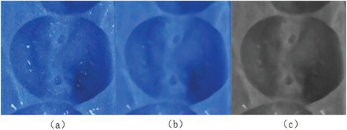
Regions of interest (ROIs) are first divided according to the bounding boxes obtained by object detection. Figure 5(a) is one of the results after object detection, whose texture and noise greatly affecting the result of edge detection. In the process of reducing noise as smooth as possible, we need to prevent edge information from being damaged by blurring, thus median filtering is chosen since its resulting image is smoother than the bilateral filtering one. Results can be seen in Figure 5(b) and (c).

Figure 5. Results of smoothing.

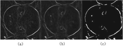
Then, the edge image of the gray image is obtained as shown in Figure 6(a). Most edges are clear, but there are still many fluffs. Bilateral filtering is used to smooth and strong edges are retained while most fluff edges are removed. The result of bilateral filtering can be computed as (2) $\begin{array}{rl}d(i,j,x,y)& =\exp \left(-\frac{{(i-x)}^2{(j-y)}^2}{2{\sigma }_d^2}\right)\end{array}$(2) (3) $\begin{array}{rl}r(i,j,x,y)& =\exp \left(-\frac{f(i,j)-f{(x,y)}^2}{2{\sigma }_r^2}\right)\end{array}$(3) (4) $\begin{array}{rl}\omega (i,j,x,y)& =d(i,j,x,y)\ast r(i,j,x,y)\end{array}$(4) (5) $\begin{array}{rl}g(i,j)& =\frac{\sum _{x,y}f(x,y)\omega (i,j,x,y)}{\sum _{x,y}\omega (i,j,x,y)}\end{array}$(5) where ${\sigma }_d$ (defining the size of the spatial neighbourhood) and ${\sigma }_r$ (controlling how much an adjacent pixel is downweighted because of the intensity difference) are smoothing parameters, $f(i,j)$ and $f(x,y)$ are the intensity of pixels $(i,j)$ and $(x,y)$ respectively, and $g(i,j)$ is the denoised intensity of pixel. Finally, we select an appropriate threshold for binarization. The results are shown in Figure 6(b) and (c), respectively.

Figure 6. Results of edge detecting.

The edge detection here only uses Sobel operator (Gonzalez & Woods, 2010) instead of Canny edge detection (Rong et al., 2014) algorithm flow. The reason is that our dental impression image has not only useless edges, but also weak edges, and the change in gray level at the border of adjacent contours is not so obvious that the result is discrete edge fragment. Directly using Canny detection is not conducive to subsequent fixing. Therefore, we use Sobel operator to obtain discrete edges and multiple methods to exclude, fit, and connect later. The Sobel gradient and direction of pixel $(x,y)$ are computed as (6) $\begin{array}{rl}G& =\sqrt{G_x^2+G_y^2}\end{array}$(6) (7) $\begin{array}{rl}\theta & =\arctan (G_y/G_x)\end{array}$(7) where $G_x$ is the horizontal gradient and $G_y$ is the vertical gradient.

2.3. Edge fragments filtering and pairing

After getting clear discrete edges, we exclude useless edges and retain the main edge fragments as many as possible, and then pair endpoints to facilitate subsequent fitting.

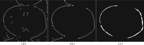
Contours of all edges are obtained and shown in Figure 7(a). We calculate the perimeter of fragments, and choose a suitable threshold, set as $\text{threshold}=(\text{median}+\mathrm{average})\text{/2}$ in this paper, to retain the edges with perimeters within $\left(\frac{\text{threshold}}{\text{2}},2\ast \text{threshold}\right)$ only. Then during the endpoints pairing, it is found that the ROI contains not only the required contour, but also parts of the two adjacent teeth, which forces us to judge the needed endpoints. As shown in Figure 7(b), if an endpoint is located within a small neighbourhood of borders, then the edge owning the endpoint is excluded. Till now, most of useless edges are filtered (as shown in Figure 7(c)).

Figure 7. Results of edge filtering.

For pairing, we divide eight directions and four quadrants according to the 8-pixel neighbourhood. For each endpoint, its extension direction is determined and the endpoint with shortest distance is searched in the quadrant that the extension direction points to. If the extension direction is exactly up, down, left or right, then search in two quadrants. The two endpoints that have been successfully paired no longer participate in the other pairing process. Finally, the unsuccessful paired point and its edge are removed.

2.4. Fitting connection

After correctly pairing, the fitting connection of the pairs appears simple. This paper uses the Bezier curve (Rababah & Jaradat, 2020) to perform the fitting.

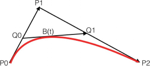
The formula of second-order Bezier curve is shown in Equation (8): (8) $B(t)=(1-t{)}^2{P}_0+2t(1-t)P_1+t^2{P}_2\text{, }t\in [0,1]$(8) where $P_0$, $P_1$ and $P_2$ are three points. Its geometric meaning is shown in Figure 8. Keeping $\frac{P_0{Q}_0}{Q_0{P}_1}=\frac{P_1{Q}_1}{Q_1{P}_2}=\frac{Q_0{B}_t}{B_t{Q}_1}$ while let $Q_0$ move from $P_0$ to $P_1$, then the motion trajectory of $B_t$ is a second-order Bezier curve.

Figure 8. The formation second-order Bezier curve.

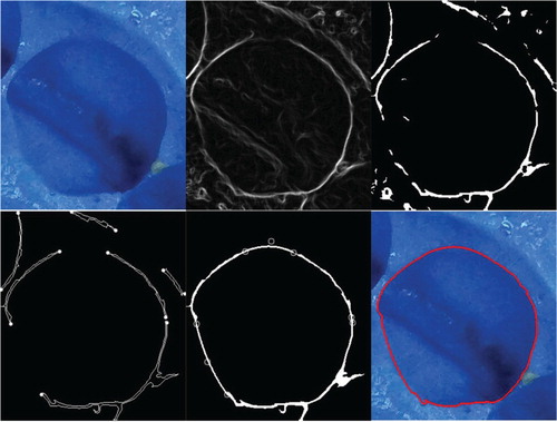
Assume two paired endpoints are $P_0$ and $P_2$, and their extension lines (tangent) intersect at point $P_1$. With the help of second-order Bezier curve, we fit a curved edge between two endpoints. The results are shown in Figure 9. If the distance between two paired endpoints is too short, connect directly with a straight line. Another complete process of a tooth mark segmentation is shown in Figure 10.

Figure 9. The result of fitting connection by Bezier curve.

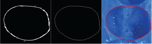
Figure 10. Another complete process of a tooth mark segmentation.

3. Contour extraction

To response the possible mistake in segmentation, an additional interface is proposed in this section. It takes segmented images, shown in Figure 1(b), as input and automatically extracts the coordinates of tooth contours. The proposed interface not only guarantees that the output from any other effective segmentation algorithms can be used directly, but also allow manual segmentation when the result of the automatic algorithm is poor.

Canny edge detection (Rong et al., 2014) is performed on the input image, as shown in Figure 11(a). Since details are poor, we perform the expansion operation (Gonzalez & Woods, 2010) to merge the discrete edges (expanding the highlighted area), and then the corrosion operation (Gonzalez & Woods, 2010) with a kernel of the same size as expansion to refine edges to minimize errors (expanding the dark part), as shown in Figure 11(b).

Figure 11. (a) The result of Canny edge detection. (b) The result of expansion and corrosion.

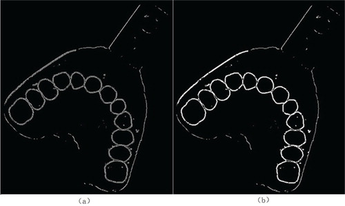
Then we extract coordinates of all inner and outer contours, and calculate their areas. After observation, we can almost determine that for our images, the contour with the eighth largest area is belong to a tooth mark. Therefore, we regard this contour area as a reference and set a threshold to exclude unnecessary contours, meanwhile taking inner contours only, and finally get the result shown in Figure 12(a). The contour area is calculated as follows: (9) $S={\int }_{xmin}^{xmax}|y_x^{\mathrm{\prime }}-y_x^{{}^{\mathrm{\prime }\mathrm{\prime }}}|dx$(9) where $y_x^{\mathrm{\prime }}$ and $y_x^{{}^{\mathrm{\prime }\mathrm{\prime }}}$ are the ordinates of two contour points whose abscissa is equal to x.

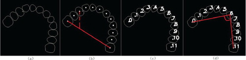
Figure 12. (a) The desired contours. (b) The auxiliary line helping numbering. (c) The result of numbering. (d) The angle feature.

The ‘small tail' in the third contour from left to right causes little errors, which can be ignored.

4. Feature extraction and matching

4.1. Numbering

In order to ensure the unification of images taken at different rotation angles, obtained contours need to be numbered first. A simple numbering algorithm is proposed, i.e. to start from 0 and number in the clockwise direction.

Since the coordinates of each contour point are saved, we calculate the first moment to obtain centroids of each contour and then the sums of distances between each centroid with all other centroids to find the two endpoints with largest sums of distances. Furthermore, the rectangular coordinate system is established to determine the starting point of the two ends. As shown in Figure 12(b), the two ends are connected to obtain a straight line. The upper-left corner of the image is chosen as the origin, the horizontal axis is the x-axis, and the vertical axis is the y-axis. Given the coordinates of the two ends, it is not difficult to get the straight line equation. Take any other point except the two ends and project the point on the straight line with a constant x value, and then their y coordinates are compared. If the y value of the point is bigger than the projected one, then all other points are above the straight line, and the left endpoint is regarded as starting point, otherwise, the right endpoint is starting point.

Figure 12(c) shows the contour after numbering. The centroid of contours is calculated as follows: (10) $\begin{array}{rl}{m}_{00}& =\sum _x\sum _y{x}^0{y}^{0}I(x,y)=\sum _x\sum _{y}I(x,y)\end{array}$(10) (11) $\begin{array}{rl}{m}_{10}& =\sum _x\sum _y{x}^1{y}^{0}I(x,y)=\sum _x\sum _{y}x\ast I(x,y)\end{array}$(11) (12) $\begin{array}{rl}{m}_{01}& =\sum _x\sum _y{x}^0{y}^{1}I(x,y)=\sum _x\sum _{y}y\ast I(x,y)\end{array}$(12) (13) $\begin{array}{rl}C& =\left(\frac{m_{10}}{m_{00}},\frac{m_{01}}{m_{00}}\right)\end{array}$(13) where $(x,y)$ is the coordinate of contour points, and $I(x,y)$ is the corresponding pixel value, which is either 0 or 1 for a binary image.

4.2. Feature extraction

Three features, four eigenvalues are chosen, i.e. the number of contours, the ratio of the largest and the smallest contour areas, and the angles formed by centroids of the two ends and front teeth, such as No. 5 and No. 6 in Figure 12(d), respectively. Areas are calculated by Equation (9), while centroids calculated by (13).

4.3. Matching function

Gaussian function is used for matching as it is a very applicable function. For examples, in the field of image processing, Gaussian blur stands up; in the field of signal processing, Gaussian filtering is used to reduce noise, and in the field of statistics, it can be used to describe normal distribution.

The one-dimensional Gaussian function is defined as (14) $f(x)=\frac{1}{\sigma \sqrt{2\pi }}{e}^{-\frac{{(x-\mu )}^2}{2{\sigma }^2}}$(14)

We construct a Gaussian function with $\mu$ set as the average of a set of $x$ and ${\sigma }^2$ the variance, so the set of $x$ is concentrated near the top peak, which also means their Gaussian function values are all above a certain percentage of the top value. Therefore, for an eigenvalue matching, we take a training set and calculate averages and variances for each person, and set a proportion of the peak value as the threshold. Then we build a database conveniently.

4.4. Identification

The proposed matching order is the number of contours, the maximum and minimum area ratio, and the angle.

After calculating three eigenvalues, as shown in Figure 13, for each dental impression in database, we compare the number first, and directly jump to the next dental impression if not matching. Then we take parameters of the feature ratio to construct its Gaussian function, and substitute the ratio into the Gaussian function to calculate the value. If it is greater than one-tenth of the maximum value of the function, match pass, otherwise, jump to the next. The angle is same as above. We finally output where the match fail or ids of successful match as results. The threshold is set as one-tenth of the peak value after repeated experiments.

Figure 13. The flow chart of identification.

5. Experiment

5.1. Dataset

The experiments were run on a computer with a CPU of 2.80 GHz, 8 GB of memory, and an operating system of 64-bit Windows 10. The software development platform is Visual Studio 2015, using OpenCV. The database currently includes a total of 50 dental impressions, which were from 50 volunteers and produced by ourselves. Each dental impression took multiple images with different rotation angles and brightness. The materials and tools used for making dental impression models are composed of dental alginate impression material powder, measuring spoon, measuring cup, spatula, mixing bowl, and dental tray. Impression materials are harmless to the human body. The collection steps are as follows: first, take two spoons of the impression powder with measuring spoon and pour it into the mixing bowl; second, take two scales of water into the impression powder and quickly stir; third, spread the stirred alginate material evenly on the dental tray; fourth, put the dental tray containing alginate material into the mouth, and the volunteer bites the dental tray, taken out after about one minute; fifth, dental impression images are obtained with a digital camera. Several collected images are shown in Figure 14.

Figure 14. Five dental impressions from different persons.

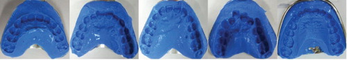
Images of 50 existing dental impressions are pre-processed to establish a database. Among them, five images of each dental impression are used to form a training set to build the database.

5.2. Indicator ROF

Generally, biometric identifications use the indicator accuracy (ACY) to evaluate results, shown as follows: (15) $ACY=\frac{\sum _M^i{\sigma }_i}{M}$(15) where $M$ is the total number of test images; ${\sigma }_i$ indicates whether the result of the i-th test image is equal to the real identity. If it is, ${\sigma }_i=1$, otherwise ${\sigma }_i=0$.

Compared with X-ray images, teeth structure features from dental impression images are unable to be matched with single tooth feature and dental works feature. Therefore, the matching result may contain multiple identity when the database is large. Actually, matching multiple identity is still of great significance to the forensic autopsy. It can exclude a large number of candidate identities and be used as an auxiliary of subsequent DNA identification. Therefore, to evaluate the proposed strategy more comprehensively, an indicator named rate of filtration (ROF) is defined as: (16) $\text{ROF}=\frac{\sum _M^i\frac{N-R_i}{N-1}\ast {\tau }_i}{M}$(16) where $M$ is the total number of test images; $N$ is the total number of dental impressions in the database; $R_i$ is the number of matching result of the i-th test image; ${\tau }_i$ indicates whether the result of the i-th test image includes the real identity, if it is, ${\tau }_i=1$, otherwise ${\tau }_i=0$.

For example, suppose there are $N$ dental impressions in the database, and $M$ images are tested. When calculating accuracy, for a test image, if the result is equal to the real identity, it is counted as $1$, otherwise it is $0$. All test results are summed and divided by the total number of test images to get the accuracy. In other words, when the test result is only the real identity, that is, when the algorithm excludes $N-1$ objects, it is counted as $1$, which is equal to $\frac{N-1}{N-1}$. Then, when the result has two identities containing the real one, $N-2$ are excluded, we can count it as $\frac{N-2}{N-1}$, and so on, finally, all test images are also summed and divided by the total number, and the ROF is obtained. It can be seen when the matching result is only one real identity or does not contain the real one, the ROF is equal to the accuracy, so the accuracy is a special case of the ROF (excluding all other objects, only the real one is left). Therefore, we can compare the ROF with the accuracy of other methods.

Of course, if there are too many result objects, it is meaningless for tooth identification. For example, when the number of matched objects is bigger than or equal to 10% of the total number of objects, it is counted as 0. In this paper, an additional ROF, that counting results with more than five objects as 0, is listed.

5.3. Comparison and analysis

After excluding bad models (No. 24, No. 32, No. 38) and bad images which are obtained incorrectly such as images shown in Figure 15, a database of 47 persons is built. Five to ten photos are chosen as test images for each dental impression, with a total number of 311. For each test image, the result includes all ids of dental impression that successfully matched. As a result, the numbers of matched ids of every test image are all in the range of 0–9.

Figure 15. (a) Tooth marks are covered. (b) Inclined tooth marks caused by incorrect bite.

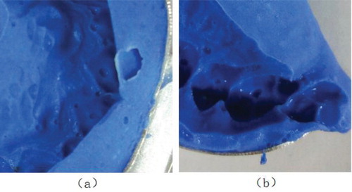
Table 1 shows the matching results and corresponding ROFs of six test images from No. 41 dental impression, whose results are quite fluctuated. As for our database with 47 objects, when the number of result objects is less than or equal to 5, ROF is bigger than 90%. From the data value (quantitative analysis), comparing the equal accuracy, 90% has reached a good matching result, and it is more objective than accuracy. From a practical sense (qualitative analysis), we can also quickly select the real identity manually from a set data of less than or equal to five, which has greatly reduced the range and achieved a good result. Therefore, the indicator ROF is valid. Table 1 also gives the total ROF of all 311 test images.

Table 1. The result ID of some test images and their ROFs.

Test image	Result ID	ROF
041_01	26, 29, 41	95.65%
041_02	10, 12, 26, 29, 41	91.30%
041_04	10, 29, 37, 41, 44, 46	89.13%
041_08	41	100%
041_09	5, 41	97.82%
041_10	NONE	0%
Total ROF_1	–	90.45%
Total ROF_2	≤ 5 objects	84.26%

The experimental results are compared with method (1) Partial bidirectional Hausdorff distance (HD) of the original contour (Zhou & Abdel-Mottaleb, 2005), (2) Partial bidirectional of the original contour Weighted Hausdorff distance (wHD) (Jain & Chen, 2004) and (3) wHD of effective contour (i.e. trimmed contour) (Lin et al., 2012). Table 2 gives a comparison with these three methods. Because dental radiographs and dental impression images are quite different, as same as the features extracted from them, it is difficult to run their methods on our data set, so the results are directly compared. Among them, test images of method (1) (2) (3) include 115 upper-jaw teeth and 105 lower-jaw teeth, while due to inconvenience in collecting dental impression models of lower-jaw teeth, we use 311 images of only upper-jaw teeth.

Table 2. Comparison of tooth matching accuracy.

		Top-N retrievals
Method	Jaw	N = 1	N = 3	N = 5	N = 10	N = 15	N = 20
Zhou and Abdel-Mottaleb (2005)	Upper	44/115	60/115	65/115	79/115	83/115	85/115
		38.20%	52.20%	56.50%	68.70%	72.20%	73.90%
	Lower	38/105	52/105	66/105	78/105	85/105	90/105
		36.20%	49.50%	62.90%	74.30%	80.90%	85.70%
Jain and Chen (2004)	Upper	47/115	77/115	87/115	95/115	98/115	98/115
		40.90%	66.90%	75.70%	82.60%	85.20%	85.20%
	Lower	39/105	60/105	69/105	79/105	88/105	91/105
		37.10%	57.10%	65.70%	75.20%	83.80%	86.70%
Lin et al. (2012)	Upper	50/115	77/115	88/115	98/115	101/115	104/115
		43.50%	66.90%	76.50%	85.20%	87.80%	90.40%
	Lower	50/105	72/105	83/105	91/105	91/105	94/105
		47.60%	68.60%	79.00%	86.70%	86.70%	89.50%
Ours	Upper	130/311	229/311	268/311	289/311	289/311	289/311
		41.80%	73.63%	86.17%	92.93%	92.93%	92.93%

The matching results of methods (1), (2) and (3) are in the form of a sequence. They calculate the distance between the test image with each person in database, the smaller the distance, the better. Top-N means that the real identity is in the first N of the result sequence, while suspected objects in our matching results have no priority. Therefore, in the same case, our accuracy will be lower than or equal to their accuracy. For example, a test image result has four objects, and the real one is ranked 3rd. For Top-3, methods (1) (2) (3) count the result as right, but we count it as wrong because the number of matched objects is four, bigger than three. Compared with accuracies in Table 2, our method is only slightly lower than method (3) when $N=1$. The reason is our overall dental structure feature cannot combine the information of the shape of a single tooth or DWs like X-rays. And in the case of multiple result objects such as $N=3,N=5$, our accuracy is higher. Results show that our method is superior to a certain degree, and the accuracy is not lower than those using X-ray images, while dental impression images are much easier to acquire in large numbers. Furthermore, as we can see, after combining both upper and lower jaws for matching, compared with single-jaw teeth matching, the accuracy of method (3) has been greatly improved, even achieving 100% for top-2. Therefore, our results of only upper-jaw teeth, whose accuracy is higher than (3), are quite encouraging. In future work, the combination of teeth matching with both upper and lower jaws shows a good potential.

We compare the ROF in Table 1 with the accuracy in Table 2. Obviously, while guaranteeing its effectiveness, ROF is more objective, and it can be easily calculated without the need for calculating different top-N to obtain the performance of the algorithm.

Table 3 shows a comparison of identity rate, indicating the correct recognition rate for all persons in the database. Instead of calculated by taking the intersection of results from different test images of the same person, we use our more objective ROF. It can be seen that compared with the learning method ToothNet (Minaee et al., 2019), ours still has something to be improved: combining with the information of lower-jaw teeth and introducing deep learning models to combine low-dimensional geometric features of this paper and high-dimensional deep features.

Table 3. Comparison of identity rate.

Method	Total person	Total images	Identity rate
Ours	47	311	90.45%
Coloured images (Cui et al., 2019)	45	90	88.88%
ToothNet (Minaee et al., 2019)	–	–	96.85%

6. Conclusion

A novel strategy of dental identification based on teeth structure features using dental impression images is proposed. For a dental impression image, it achieves tooth marks detection, tooth contours locating segmentation, teeth structure features extraction and identification. To automatically segment tooth contours, a feasible method through tooth marks detection, Sobel operator, edge filtering, endpoints pairing and Bezier curve fitting connection is proposed. For possibly poor segmentations, a universal interface is designed, which takes a contoured image as input. For the selection and matching of features, this paper proposes two geometric features and implements a matching strategy. Finally, we propose a novel indicator named rate of filtration (ROF), and prove its objectivity and efficiency. Experiment containing 47 persons comprised of 311 images shows a ROF of 90.45% while using only upper-jaw teeth. In comparison, only the top-1 matching accuracy is slightly lower than methods using dental radiographs, while the overall accuracy of the proposed method relatively higher, which is encouraging. Meanwhile, according to the result that when combining both upper and lower jaw teeth to match the accuracy is greatly improved, our proposed method is full of prospects and potentials.

At the same time, there are still chances for improvement. The size of our dental impression database is not large enough. In addition, the proposed method for dental impression segmentation is quite dependent on precise tooth marks detection and endpoints pairing, which is not robust enough. Also, selected features are low-dimensional and not unique enough. The future work will also focus on these shortcomings, as well as combining some learning-based deep features.

Acknowledgements

This work is supported by the National Natural Science Foundation of China (Nos. 61771430, 61573316, 61873082), the Zhejiang Provincial Natural Science Foundation (No. LY20F020022), the National Key R&D Program of China (No. 2018YFB0204003) and the Zhejiang University Student Science and Technology Innovation Activity (No. 2019R403070).

Disclosure statement

No potential conflict of interest was reported by the authors.

Additional information

Funding

This work is supported by the National Natural Science Foundation of China [grant numbers 61771430, 61573316, 61873082], the Zhejiang Provincial Natural Science Foundation [grant number LY20F020022], the National Key R&D Program of China [grant number 2018YFB0204003] and the Zhejiang University Student Science and Technology Innovation Activity [grant number 2019R403070].

Appendix

Table

Algorithm 1 The framework of the proposed strategy.
Input:
$I(x,y)$: the dental impression image
$netweights$: a trained model of SSD network
Output: $Matc{h}_{-}Id$, $Fai{l}_{-}Step$
1: Detect tooth mark objects of $I(x,y)$ by SSD.
Using the model $netweights$ and get a set of bounding boxes $bboxes$ of every single tooth.
2: for $bbox$ in $bboxes$
3:  Using median filtering smooth the ROI ($bbox$).
4:  Get the edge image of the ROI after smoothing and graying using Sobel with equations (6) and (7).
5:  Using bilateral filtering with equation (5) smooth the above ROI and binary it.
6:  Get main edge fragments and pairing their endpoints.
7:  Using equation (8) connect paired endpoints and get the contour of the single tooth mark.
8: end for
9: Get a set of contours $teethct$.
10: Calculate geometric features $f_1,f_2,f_3,f_3$ with equations (9) and (13).
11: for $id=n$ in $Database$
12:  Get the matching functions of $f_1^n,f_2^n,f_3^n,f_4^n$ with equation (14).
13:  Compare $f_1,f_2,f_3,f_3$ with $f_1^n,f_2^n,f_3^n,f_4^n$.
14:  Save the failed feature in $Fai{l}_{-}Step$ if the match fails.
15:  Save the $n$ in $Matc{h}_{-}Id$ if match successfully.
16: end for
17: return $Matc{h}_{-}Id$, $Fai{l}_{-}Step$

References

- Badrinarayanan, V., Kendall, A., & Cipolla, R. (2017). Segnet: A deep convolutional encoder-decoder architecture for image segmentation. IEEE Transactions on Pattern Analysis and Machine Intelligence, 39(12), 2481–2495. https://doi.org/10.1109/TPAMI.2016.2644615
- Banday, M., & Mir, A. H. (2019, October). Dental biometric identification system using AR model. In TENCON 2019-2019 IEEE Region 10 Conference (TENCON) (pp. 2363–2369). IEEE.
- Chen, H., & Jain, A. K. (2005). Dental biometrics: Alignment and matching of dental radiographs. IEEE Transactions on Pattern Analysis and Machine Intelligence, 27(8), 1319–1326. https://doi.org/10.1109/TPAMI.2005.157
- Chen, L. C., Papandreou, G., Kokkinos, I., Murphy, K., & Yuille, A. L. (2017). Deeplab: Semantic image segmentation with deep convolutional nets, atrous convolution, and fully connected CRFs. IEEE Transactions on Pattern Analysis and Machine Intelligence, 40(4), 834–848. https://doi.org/10.1109/TPAMI.2017.2699184
- Cui, Z., Li, C., & Wang, W. (2019). ToothNet: automatic tooth instance segmentation and identification from cone beam CT images. In Proceedings of the IEEE Conference on Computer Vision and Pattern Recognition (pp. 6368–6377).
- Fahmy, G., Nassar, D., Haj-Said, E., Chen, H., Nomir, O., Zhou, J., & Jain, A. K. (2004, July). Towards an automated dental identification system (ADIS). In International conference on biometric authentication (pp. 789–796). Springer.
- Gonzalez, R. C., & Woods, R. E. (2010). Digital image processing (3rd ed.). Person Education Press.
- Hofer, M., & Marana, A. N. (2007, October). Dental biometrics: human identification based on dental work information. In XX Brazilian Symposium on Computer Graphics and Image Processing (SIBGRAPI 2007) (pp. 281–286). IEEE.
- Jader, G., Fontineli, J., Ruiz, M., Abdalla, K., Pithon, M., & Oliveira, L. (2018, October). Deep instance segmentation of teeth in panoramic X-ray images. In 2018 31st SIBGRAPI Conference on Graphics, Patterns and Images (SIBGRAPI) (pp. 400–407). IEEE.
- Jain, A. K., & Chen, H. (2004). Matching of dental X-ray images for human identification. Pattern Recognition, 37(7), 1519–1532. https://doi.org/10.1016/j.patcog.2003.12.016
- Jampani, V., Kiefel, M., & Gehler, P. V. (2016). Learning sparse high dimensional filters: Image filtering, dense crfs and bilateral neural networks. In Proceedings of the IEEE Conference on Computer Vision and Pattern Recognition (pp. 4452–4461).
- Krizhevsky, A., Sutskever, I., & Hinton, G. E. (2012). Imagenet classification with deep convolutional neural networks. In Advances in neural information processing systems 25 (pp. 1097–1105).
- Kumar, R. (2016, October). Teeth recognition for person identification. In 2016 International Conference on Computation System and Information Technology for Sustainable Solutions (CSITSS) (pp. 13–16). IEEE.
- Lin, G., Milan, A., Shen, C., & Reid, I. (2017). Refinenet: Multi-path refinement networks for high-resolution semantic segmentation. In Proceedings of the IEEE conference on computer vision and pattern recognition (pp. 1925–1934).
- Lin, P. L., Lai, Y. H., & Huang, P. W. (2010). An effective classification and numbering system for dental bitewing radiographs using teeth region and contour information. Pattern Recognition, 43(4), 1380–1392. https://doi.org/10.1016/j.patcog.2009.10.005
- Lin, P. L., Lai, Y. H., & Huang, P. W. (2012). Dental biometrics: Human identification based on teeth and dental works in bitewing radiographs. Pattern Recognition, 45(3), 934–946. https://doi.org/10.1016/j.patcog.2011.08.027
- Liu, W., Anguelov, D., Erhan, D., Szegedy, C., Reed, S., Fu, C. Y., & Berg, A. C. (2016, October). Ssd: Single shot multibox detector. In European conference on computer vision (pp. 21–37). Springer.
- Long, J., Shelhamer, E., & Darrell, T. (2015). Fully convolutional networks for semantic segmentation. In Proceedings of the IEEE conference on computer vision and pattern recognition (pp. 3431–3440).
- Minaee, S., Abdolrashidi, A., Su, H., Bennamoun, M., & Zhang, D. (2019). Biometric recognition using deep learning: A survey. arXiv preprint arXiv:1912.00271.
- Nomir, O., & Abdel-Mottaleb, M. (2005). A system for human identification from X-ray dental radiographs. Pattern Recognition, 38(8), 1295–1305. https://doi.org/10.1016/j.patcog.2004.12.010
- Nomir, O., & Abdel-Mottaleb, M. (2007). Human identification from dental X-ray images based on the shape and appearance of the teeth. IEEE Transactions on Information Forensics and Security, 2(2), 188–197. https://doi.org/10.1109/TIFS.2007.897245
- Nomir, O., & Abdel-Mottaleb, M. (2008a). Fusion of matching algorithms for human identification using dental X-ray radiographs. IEEE Transactions on Information Forensics and Security, 3(2), 223–233. https://doi.org/10.1109/TIFS.2008.919343
- Nomir, O., & Abdel-Mottaleb, M. (2008b). Hierarchical contour matching for dental X-ray radiographs. Pattern Recognition, 41(1), 130–138. https://doi.org/10.1016/j.patcog.2007.05.015
- Rababah, A., & Jaradat, M. (2020). Approximating offset curves using bézier curves with high accuracy. International Journal of Electrical & Computer Engineering, 10, 2088–8708. doi: 10.11591/ijece.v10i2.pp1648-1654.
- Rajput, P., & Mahajan, K. J. (2016, December). Dental biometric in human forensic identification. In 2016 International Conference on Global Trends in Signal Processing, Information Computing and Communication (ICGTSPICC) (pp. 409–413). IEEE.
- Rehman, F., Akram, M. U., Faraz, K., & Riaz, N. (2015, April). Human identification using dental biometric analysis. In 2015 Fifth International Conference on Digital Information and Communication Technology and its Applications (DICTAP) (pp. 96–100). IEEE.
- Rong, W., Li, Z., Zhang, W., & Sun, L. (2014, August). An improved CANNY edge detection algorithm. In 2014 IEEE International Conference on Mechatronics and Automation (pp. 577–582). IEEE.
- Uijlings, J. R., Van De Sande, K. E., Gevers, T., & Smeulders, A. W. (2013). Selective search for object recognition. International Journal of Computer Vision, 104(2), 154–171. https://doi.org/10.1007/s11263-013-0620-5
- Yang, Z. B., Radzienski, M., Kudela, P., & Ostachowicz, W. (2016). Scale-wavenumber domain filtering method for curvature modal damage detection. Composite Structures, 154, 396–409. https://doi.org/10.1016/j.compstruct.2016.07.074
- Zhou, J., & Abdel-Mottaleb, M. (2005). A content-based system for human identification based on bitewing dental X-ray images. Pattern Recognition, 38(11), 2132–2142. https://doi.org/10.1016/j.patcog.2005.01.011