Active disturbance rejection switching control of quadrotor based on robust differentiator

Abstract

To solve the problem of trajectory tracking control of a quadrotor unmanned aerial vehicle (UAV) under white noise disturbance, a new active disturbance rejection control (ADRC), an active disturbance rejection switching control (ADRSC) algorithm of the quadrotor based on a robust differentiator, is proposed. The dynamic model of the quadrotor is stated in three sub-equations, and a control algorithm is designed. The exact robust differentiator (ERD) replaces the tracking differentiator in the traditional ADRC algorithm to improve the accuracy and robustness of the differential signal. The ADRSC algorithm controls the quadrotor to improve its anti-white-noise disturbance ability and control accuracy. Simulation results show that the quadrotor has an anti-white-noise disturbance ability of no more than 0.1 dB intensity with this algorithm.

KEYWORDS:

• Quadrotor unmanned aerial vehicle (UAV)
• robust differentiator
• active disturbance rejection control (ADRC)
• trajectory tracking control

Introduction

The quadrotor unmanned aerial vehicle (UAV) is a rotorcraft that can perform three kinds of attitude changes: vertical takeoff and landing, pitch roll, and yaw. Compared to fixed-wing and other single-rotor flight vehicles, the quadrotor UAV has a simple structure, high payload, and strong maneuverability. The quadrotor UAV has the characteristics of under-actuation, nonlinearity, and strong coupling. These characteristics bring a great difficulty to its control, especially under an external disturbance. The body of the quadrotor UAV is light, and it easily suffers from disturbance. The attitude and position of the quadrotor UAV during the state feedback control process also faces white noise disturbance.

Proportion integral derivative (PID) control is widely used in quadrotor UAVs, but due to the vehicle’s nonlinear characteristics, PID control cannot produce good system performance in complex environments (Khatoon et al., 2014). Su et al. (2011) proposed a nonlinear PID method to control a quadrotor UAV, but the dynamic model did not fully consider the dynamic characteristics. An adaptive sliding mode control (SMC) algorithm was proposed based on immersion and invariant theory, with verified anti-interference ability under periodic disturbance (Xia et al., 2017). Chen et al. (2016) designed a backstep sliding mode controller and a robust SMC observer for a quadrotor UAV and verified the robustness of the algorithm and the accuracy of the observer by gradually increasing the disturbance. Lee et al. (2009) designed the controller of a quadrotor based on feedback linearization theory and compared the control performance of two methods of adaptive sliding mode control and feedback linearization control. An SMC algorithm has strong anti-interference and robustness. Other nonlinear SMC algorithms were designed for the control of a quadrotor UAV (Chen et al., 2015; Dolatabadi & Yazdanpanah, 2015; Han, 1998; Wang et al., 2016). However, the form of an SMC algorithm is often complicated, which is not conducive to the streamlined design of the control law. Therefore, it is necessary to find a simple and efficient control algorithm that has the characteristics of anti-disturbance and robustness. Huang (2019) investigated for a class of discrete time-varying systems with censored measurements and parameter uncertainties. Shen (2019) design a finite-horizon filter such that an upper bound is guaranteed and the filter gain minimizing such an upper bound is subsequently obtained in terms of the solution to a set of recursive equations. Active disturbance rejection control (ADRC) is an anti-disturbance control algorithm (Han, 1998). The use of errors and nonlinear functions can improve the overall performance of control in actual production processes. Liu et al. (2015) and Wu et al. (2016) researched and applied ADRC algorithms in quadrotors. In the original ADRC, the tracking differentiator (TD) is a relatively independent part that is used to extract the differential signal and reduce the interference of external noise (Han & Wang, 1994). The speed and accuracy of the ADRC is determined by the accuracy of the differential signal extracted by the TD and its anti-disturbance performance. Extended state observer (ESO) is a state observer based on error variation (Han, 1995). An ESO can be categorized as either a linear extended state observer (LESO) or nonlinear extended state observer (NLESO), each with its own advantages and characteristics. Switching control based on ADRC was proposed (Li et al., 2016b); a linear active disturbance rejection control/nonlinear active disturbance rejection control (LADRC/NLADRC) algorithm combines the advantages of both. Proof of stability is provided based on the example of a single-input single-output (SISO) system. The active disturbance rejection switching control (ADRSC) algorithm is an enrichment of the ADRC algorithm that is more stable and robust.

Therefore, to improve the anti-disturbance ability of the whole control process of the quadrotor, an ADRSC algorithm based on a robust differentiator is proposed. The robust differentiator is used as the scheduling transition process in ADRC. Based on the traditional ADRC, LADRC/NLADRC switching is adopted, and the stability analysis of the switching control is undertaken. The trajectory tracking control performance of the quadrotor based on the traditional differentiator and the robust differentiator in a white noise disturbance environment is compared, and the anti-disturbance and robustness of the control algorithm are verified.

Dynamic modelling of quadrotor

According to the literature (Wang et al., 2016; Wu et al., 2016), the quadrotor dynamic model has the form (1) $\{\begin{array}{l}\ddot{x}=u_{\tau }(\cos \phi \sin \theta \cos \psi +\sin \phi \sin \psi )/m\\ -({\kappa }_x\dot{x}/m)+d_x\\ \ddot{y}=u_{\tau }(\cos \phi \sin \theta \sin \psi -\sin \phi \cos \psi )/m\\ -({\kappa }_y\dot{y}/m)+d_y\\ \ddot{z}=u_{\tau }(\cos \phi \cos \theta )/m-g-({\kappa }_z\dot{z}/m)+d_z\\ \ddot{\phi }=l{u}_{\phi }/J_{\phi }+d_{\phi }-(l{\kappa }_{\phi }\dot{\phi }/J_{\phi })\\ \ddot{\theta }=l{u}_{\theta }/J_{\theta }+d_{\theta }-(l{\kappa }_{\theta }\dot{\theta }/J_{\theta })\\ \ddot{\psi }=u_{\psi }/J_{\psi }+d_{\psi }-({\kappa }_{\psi }\dot{\psi }/J_{\psi })\end{array}$(1) where m is the quality of the quadrotor UAV; $(x,y,z{)}^T$ is the current position; $(\phi ,\theta ,\psi {)}^T$ corresponds to the roll, pitch, and yaw (RPY) attitude angles; the three equations of $(x,y,z{)}^T$ constitute the position subsystem; the three equations of $(\phi ,\theta ,\psi {)}^T$ constitute the attitude subsystem; $({\kappa }_x,{\kappa }_y,{\kappa }_z,{\kappa }_{\phi },{\kappa }_{\theta },{\kappa }_{\psi }{)}^T$ is the damping coefficient group of the system; l is the length of the quadrotor wing; $(d_x,d_y,d_z,d_{\phi },d_{\theta },d_{\psi }{)}^T$ consists of the perturbation amounts of each channel; and g is the acceleration of gravity. The flight principle of the quadrotor is shown in Figure 1.

Figure 1. Flight principle of quadrotor unmanned aerial vehicle (UAV).

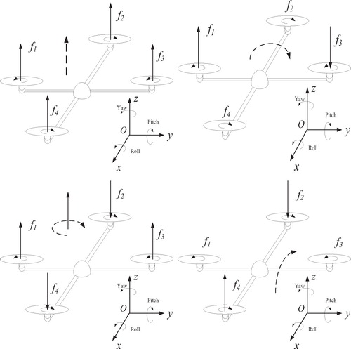
Four motor inputs are (2) $\{\begin{array}{l}{u}_{\tau }=f_1+f_2+f_3+f_4\\ u_{\phi }=-f_1-f_2+f_3+f_4\\ u_{\theta }=-f_1+f_2+f_3-f_4\\ u_{\psi }=c(f_1-f_2+f_3-f_4)\end{array}$(2) where $(u_{\tau },u_{\phi },u_{\theta },u_{\psi }{)}^T$ is the output of the controller, $(f_1,f_2,f_3,f_4{)}^T$ consists of the lift generated by the rotation of the four motors, and c is the proportional coefficient between yaw dynamic torque and lift. When keeping the speeds of the two motors unchanged, changing the speed of the other two motors can change the attitude of the quadrotor UAV. For example, if we keep the speeds of motors 1 and 3 unchanged, changing the speed of motors 2 and 4 causes $f_2$ and $f_4$ to change, so as to realize the pitch motion of the quadrotor UAV.

Since the quadrotor dynamic model contains two non-integrity constraints, the full six degrees of freedom of motion cannot be achieved. By reversing the position information of the expected trajectory of the attitude (Wang et al., 2018), the attitude angle is tracked to the expected $({\phi }_d,{\theta }_d{)}^T$: (3) $\{\begin{array}{l}{\theta }_d=\arctan \left({\displaystyle \frac{(v_p-d_p)(e_1\cos \psi +e_2\sin \psi )}{e_3{v}_p-e_3{d}_p}}\right)\\ {\phi }_d=\arcsin \left({\displaystyle \frac{(v_p-d_p)(-e_1\sin \psi +e_2\cos \psi )}{\sqrt{{(v_p-d_p)}^T(v_p-d_p)}}}\right)\end{array}$(3) where $v_p=(\ddot{x},\ddot{y},\ddot{z}+g{)}^T$, $d_p=(d_x,d_y,d_z{)}^T$. The unit vectors $\{e_1,e_2,e_3\}$ correspond to $\{(1,0,0),(0,1,0),(0,0,1)\}$.

To simplify and improve the efficiency of the control, Equation (1) is decomposed into the following form without loss of generality in the form of the state space. Define $x_1=(x,y{)}^T$, $x_2=(\dot{x},\dot{y}{)}^T$, $x_3=(\phi ,\theta {)}^T$, $x_4=(\dot{\phi },\dot{\theta }{)}^T$, $x_5=(z,\psi {)}^T$, $x_6=(\dot{z},\dot{\psi }{)}^T$. The sub-equations of the position, attitude, and altitude, respectively, of the quadrotor are (4) $\begin{array}{rl}\left(\begin{array}{c}{\dot{x}}_1\\ {\dot{x}}_2\end{array}\right)& =\left(\begin{array}{cc}{O}_{2\times 2}& I_{2\times 2}\\ A_{11}& A_{12}\end{array}\right)\left(\begin{array}{c}{x}_1\\ x_2\end{array}\right)\left(\begin{array}{c}{O}_{2\times 2}\\ B_{11}\end{array}\right)u_1+\left(\begin{array}{c}{O}_{2\times 2}\\ I_{2\times 2}\end{array}\right)d_1\end{array}$(4) (5) $\begin{array}{rl}\left(\begin{array}{c}{\dot{x}}_3\\ {\dot{x}}_4\end{array}\right)& =\left(\begin{array}{cc}{O}_{2\times 2}& I_{2\times 2}\\ A_{21}& A_{22}\end{array}\right)\left(\begin{array}{c}{x}_3\\ x_4\end{array}\right)+\left(\begin{array}{c}{O}_{2\times 2}\\ B_{21}\end{array}\right)u_2+\left(\begin{array}{c}{O}_{2\times 2}\\ I_{2\times 2}\end{array}\right)d_2\end{array}$(5) (6) $\begin{array}{rl}\left(\begin{array}{c}{\dot{x}}_5\\ {\dot{x}}_6\end{array}\right)& =\left(\begin{array}{cc}{O}_{2\times 2}& I_{2\times 2}\\ A_{31}& A_{32}\end{array}\right)\left(\begin{array}{c}{x}_5\\ x_6\end{array}\right)+\left(\begin{array}{c}{O}_{2\times 2}\\ B_{31}\end{array}\right)u_3+{\tilde{d}}_3\end{array}$(6)

The system matrices are

$A_{i1}=diag\{a_{i1},a_{i2}\}$, $A_{i2}=diag\{a_{i3},a_{i4}\}.$ where $a_{i1}=a_{i2}=0$, $a_{13}=-{\kappa }_x/m$, $a_{14}=-{\kappa }_y/m$, $a_{33}=-{\kappa }_z/m$, $a_{23}=-l{\kappa }_{\phi }/J_{\phi }$, $a_{24}=-l{\kappa }_{\theta }/J_{\theta }$, $a_{34}=-{\kappa }_{\psi }/J_{\psi }$, $i=1,2,3.$

The input matrix is $B_{i1}=diag\{b_{i1},b_{i2}\}$ $i=1,2,3.$ where $b_{32}=1/J_{\psi }$, $b_{31}=\cos \phi \cos \theta /m$, $b_{11}=(\cos \phi \sin \theta \cos \psi +\sin \phi \sin \psi )/m$, $b_{21}=l/J_{\phi }$, $b_{12}=(\cos \phi \sin \theta \sin \psi -\sin \phi \cos \psi )/m$, $b_{22}=l/J_{\theta }$.

The external disturbance vectors are $d_1=(d_x,d_y{)}^T$, $d_2=(d_{\phi },d_{\theta }{)}^T$, ${\tilde{d}}_3=(g^{\mathrm{\prime }},d_3{)}^T$, $g^{\mathrm{\prime }}=(0,g{)}^T$, $d_3=(d_z,d_{\psi }{)}^T$. $O_{2\times 2}$ is a second-order zero matrix, and $I_{2\times 2}$ is a second-order identity matrix. The control vectors are $u_1=(u_{\tau },u_{\tau }{)}^T$, $u_2=(u_{\phi },u_{\theta }{)}^T$, $u_3=(u_{\tau },u_{\psi }{)}^T$.

Remark 2.1:

Three decomposed sub-equations facilitate the implementation of the control algorithm when linear control law is employed. However, the control is still implemented in the form of a general nonlinear system. The form of the quadrotor dynamic equation can be controlled according to the above expression when the nonlinear control law is adopted.

Active disturbance rejection switching control based on robust differentiator

In this section, an active disturbance rejection switching control based on a robust differentiator is proposed. It is used for accurate position trajectory tracking control of the quadrotor. The robust differentiator solves the noise interference of the quadrotor, which has a strong ability to accurately obtain differential signals and filter out external white noise disturbance. The ADRSC algorithm enables the quadrotor to track the reference input $\{x_d,y_d,z_d,{\psi }_d\}$ for trajectory tracking control.

Robust differentiator

The traditional higher-order differentiator (Levant, 2005) is not generally strong to signal immunity and robustness, so it is necessary to find a higher-order robustness differentiator to replace the traditional TD function.

An arbitrary-order exact robust differentiator (ERD) (Levant & Livne, 2012) was proposed. The ERD features optimal asymptotics with respect to input noises and can be used for numerical differentiation as well. Compared to the original higher-order differentiator, ERD draws on the design of the higher-order sliding mode. The design idea of a second-order sliding mode is shown in Figure 2.

Figure 2. Second-order sliding mode.

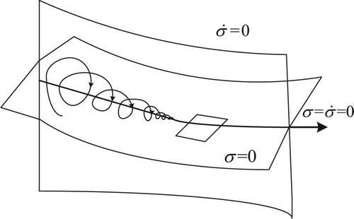
The second-order differentiator (Bartolini et al., 1999) is (7) $\{\begin{array}{l}{\dot{r}}_0=v_0,v_0=-{\lambda }_0|r_0-f(t){|}^{\frac{2}{3}}\text{ sign }(r_0-f(t))+r_1\\ {\dot{r}}_1=v_1,v_1=-{\lambda }_1|r_1-v_0{|}^{\frac{1}{2}}\text{ sign }(r_1-v_0)+r_2\\ {\dot{r}}_2=-{\lambda }_2\text{ sign }(r_2-v_1)\end{array}$(7) where $r_0$, $r_1$, $r_2$ is the observation of the second-order differentiator and $f(t)$, $v_0$, $v_1$ is a noise-disturbing input signal.

Remark 3.2:

The second-order differentiator is widely used in engineering applications. For the position information of a quadrotor, the first-order signal is its speed, and the second-order signal is its acceleration. How to accurately extract the differential signal is to ensure that the extraction process of the differential signal is not or less affected by external disturbances.

Similarly, a second-order differentiator can be generalized to an nth-order differentiator. The only requirement is that the resulting systems be homogeneous in the sense described below. The nth-order differentiator is (8) $\{\begin{array}{l}{\dot{r}}_0=v_0\\ v_0=-{\lambda }_0|r_0-f(t){|}^{\frac{n}{n+1}}\text{ sign }(r_0-f(t))+r_1\\ {\dot{r}}_1=v_1\\ v_1=-{\lambda }_1|r_1-v_0{|}^{\frac{n-1}{n}}\text{ sign }(r_1-v_0)+r_2\\ ⋮\\ {\dot{r}}_{n-1}=v_{n-1}\\ v_{n-1}=-{\lambda }_{n-1}|r_{n-1}-v_{n-2}{|}^{\frac{1}{2}}\text{ sign }(r_{n-1}-v_{n-2})+r_n\\ {\dot{r}}_n=-{\lambda }_n\text{ sign }(r_n-v_{n-1})\end{array}$(8) where $\{r_0,\cdots ,r_k\}$ is the observation of the differentiator and $\{v_0,\cdots ,v_n,f(t)\}$ is the noise-disturbing input signal of Equation (8). For any $\xi ,\gamma \in \mathbb{R}$, define $\lfloor \omega {\rfloor }^{\gamma }=|\omega {|}^{\gamma }sign(\omega )$ if $\gamma >0$ or $\xi \ne 0$.

Let $\lfloor \xi {\rfloor }^0=sign(\xi )$. For $f(t),f:\mathbb{R}\to \mathbb{R}$ is n times continuously differentiable, $n\ge 0$, $f^{(n)}$ being the Lipschitz constant with $|f^{(n+1)}|\le L$. The nth-order ERD can be described by the Filippov differential theory (Filippov, 2013), (9) $\{\begin{array}{l}{\dot{r}}_0=-{\lambda }_n{L}^{\frac{1}{n+1}}\lfloor r_0-f(t){\rfloor }^{\frac{n}{n+1}}+r_1\\ {\dot{r}}_1=-{\lambda }_{n-1}{L}^{\frac{2}{n+1}}\lfloor r_0-f(t){\rfloor }^{\frac{n-1}{n+1}}+r_2\\ ⋮\\ {\dot{r}}_{n-1}=-{\lambda }_1{L}^{\frac{n}{n+1}}\lfloor r_0-f(t){\rfloor }^{\frac{1}{n+1}}+r_n\\ {\dot{r}}_n=-{\lambda }_{0}L\text{ sign }(r_0-f(t))\end{array}$(9) where L is the Lipschitz constant, L > 0, and the value of L is proportional to the change of the disturbance. The selection of the parameter λ is ${\lambda }_i=1,1,2,3,5,8,\cdots$ or ${\lambda }_i=1.1,1.5,3,5,8,12,\cdots$.

Lemma 3.1:

(Filippov, 2013): The parameters being properly chosen, the following equalities are true in the absence of input noises after a finite time of a transient process: (10) $r_0=f_0(t);r_i=v_{i-1}=f_0^{(i)}(t),i=1,\cdots ,n$(10)

Lemma 3.2:

(Levant, 2003): Let the input noise satisfy the inequality $|f(t)-f_0(t)|\le \epsilon$. Then the following inequalities are established in finite time for some positive constants ${\mu }_i$, $v_i$, depending exclusively on the parameters of the differentiator: (11) $\{\begin{array}{l}|r_i-f_0^{(i)}(t)|\le {\mu }_i{\epsilon }^{(n-i+1)/(n+1)},i=0,\cdots ,n\\ |v_i-f_0^{(i+1)}(t)|\le v_i{\epsilon }^{(n-i)/(n+1)},i=0,\cdots ,n-1\end{array}$(11) If the solution of the dynamic system (10) is stable in the sense of Lyapunov, and then selects a reasonable parameter in (11) guarantees the homogeneity of the robust differentiator and convergence.

Active disturbance rejection switching control

The ADRC algorithm is mainly composed of TD, ESO, and a feedback control law (Chen et al., 2014). The traditional TD is replaced by ERD in this paper’s ADRC algorithm.

The ADRSC algorithm selects one of the two control states, LESO and NLESO, in different control processes according to the actual operation of the system. If the tracking performance of the system hardly changes with the disturbance amplitude, then the LESO method will improve the control efficiency. When the parameters of the system are disturbed, NLESO can suppress the negative impact of complex disturbances on the control process.

The error convergence rate of LESO is faster than that of NLESO when the total operating time t < T (transition process time) or total disturbance $|z_{n+1}(t)|>M$ (M is the upper disturbance value) or the ESO error $|e|>1$.

Define the switching condition as (12) $q=\{\begin{array}{l}1,\text{ if }t>T\wedge |e|>1\wedge |z_{n+1}(t)|>M\\ 0,\text{ else}\end{array}$(12)

When $q=1$, LESO is (13) $\{\begin{array}{l}e=z_1-y\\ {\dot{z}}_1=z_2-{\beta }_{01}e\\ {\dot{z}}_2=z_3-{\beta }_{02}e\\ ⋮\\ {\dot{z}}_n=z_{n+1}-{\beta }_{0n}e+bu\\ {\dot{z}}_{n+1}=-{\beta }_{0(n+1)}e\end{array}$(13)

The control law under LESO is (14) $u_0=\sum _{i=1}^n{k}_i(v_i-z_i)$(14)

When the switching condition $q=0$, NLESO is (15) $\{\begin{array}{l}e=z_1-y\\ {\dot{z}}_1=z_2-{\beta }_1\cdot {\phi }_1(e)\\ {\dot{z}}_2=z_3-{\beta }_2\cdot {\phi }_2(e)\\ ⋮\\ {\dot{z}}_n=z_{n+1}-{\beta }_n\cdot {\phi }_n(e)+bu\\ {\dot{z}}_{n+1}=-{\beta }_{n+1}\cdot {\phi }_{n+1}(e)\end{array}$(15) where (16) $\begin{array}{rl}{\phi }_i(e)& =fal(e,{\alpha }_i,{\delta }_i)\\ & =\{\begin{array}{l}({\alpha }_i-1){\delta }_i^{{\alpha }_i-3}{e}^3-({\alpha }_i-1){\delta }_i^{{\alpha }_i-2}{e}^2\text{ sign }(e)\\ +{\delta }_i^{{\alpha }_i-1}e,|e|\le {\delta }_i\\ |e{|}^{{\alpha }_i}\text{ sign }(e)\text{ ,}|e|>{\delta }_i\end{array}\end{array}$(16)

The control law under NLESO is (17) $u_0=\sum _{i=1}^n{k}_i\text{ fal}(v_i-z_i,{{\alpha }^{\mathrm{\prime }}}_i,{{\delta }^{\mathrm{\prime }}}_i)$(17) where the output of LESO and NLESO is $z_i(i=1,\cdots ,n+1)$; ${\beta }_{oi}(i=1,\cdots ,n+1)$ is the observation gain of LESO; ${\beta }_i(i=1,\cdots ,n+1)$ is the observation gain of NLESO; e is the observation error; ${\phi }_i(e)(i=1,\cdots ,n+1)$ is the nonlinear error function; ${\alpha }_i,{\delta }_i,{\alpha }_i^{\mathrm{\prime }},{\delta }_i^{\mathrm{\prime }}(i=1,\cdots ,n+1)$ is a tunable parameter in the fal function in Equation (17); b is the external gain of the control law; and $k_i$ is the internal gain of the control law.

Designing ESO for sub-equations of the quadrotor: (18) $\begin{array}{l}e=z_1-y\\ {\dot{z}}_1=z_2-{\beta }_1\cdot {\phi }_1(e)\\ {\dot{z}}_2=z_3-{\beta }_2\cdot {\phi }_2(e)+bu\\ {\dot{z}}_3=-{\beta }_3\cdot {\phi }_3(e)\end{array}$(18) else if q_i = 1 (19) $\begin{array}{l}e=z_1-y\\ {\dot{z}}_1=z_2-{\beta }_{01}e\\ {\dot{z}}_2=z_3-{\beta }_{02}e+bu\\ {\dot{z}}_3=-{\beta }_{03}e\end{array}$(19) $q_i$ is the switching condition of the i-th sub-equation, for $i(i=1,2,3)$ corresponding to the sub-equations of the position, attitude, and altitude, respectively, of the quadrotor. Then the virtual control law of sub-Equations (4), (5), (6) is (20) $u_{oi}=\{\begin{array}{l}\left(\begin{array}{c}{k}_{1(x,\phi ,z)}^i\text{ fal}(v_1-z_1,{{\alpha }^{\mathrm{\prime }}}_1,{{\delta }^{\mathrm{\prime }}}_1)\\ +k_{2(x,\phi ,z)}^i\text{ fal}(v_2-z_2,{{\alpha }^{\mathrm{\prime }}}_2,{{\delta }^{\mathrm{\prime }}}_2)\\ k_{1(y,\theta ,\psi )}^i\text{ fal}(v_1-z_1,{{\alpha }^{\mathrm{\prime }}}_1,{{\delta }^{\mathrm{\prime }}}_1)\\ +k_{2(y,\theta ,\psi )}^i\text{ fal}(v_2-z_2,{{\alpha }^{\mathrm{\prime }}}_2,{{\delta }^{\mathrm{\prime }}}_2)\end{array}\right),q_i=1\\ \left(\begin{array}{c}{k}_{1(x,\phi ,z)}^i(v_1-z_1)+k_{2(x,\phi ,z)}^i(v_2-z_2)\\ k_{1(y,\theta ,\psi )}^i(v_1-z_1)+k_{2(y,\theta ,\psi )}^i(v_2-z_2)\end{array}\right),q_i=0\end{array}$(20) where the internal gain of the control law is $k_{1(x,\phi ,z)}^1$, $k_{2(x,\phi ,z)}^1$, $k_{1(y,\theta ,\psi )}^i$, $k_{2(y,\theta ,\psi )}^i(i=1,2,3)$.

Then the ADRSC law of the sub-equation is (21) $u_i=\frac{u_{0i}-z_3}{b}(i=1,2,3)$(21)

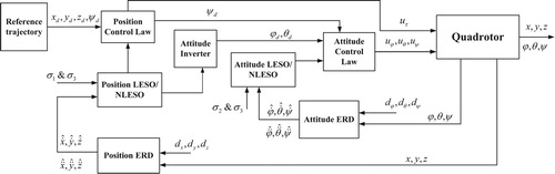
The block diagram of the ADRSC structure is shown in Figure 3. The robust differentiator is located before the attitude control law and is used to obtain the estimated values $(\hat{\dot{\phi }},\hat{\dot{\theta }},\hat{\dot{\psi }})$ and $(\hat{\ddot{\phi }},\hat{\ddot{\theta }},\hat{\ddot{\psi }})$ of the differential signals of the attitude angle $(\phi ,\theta ,\psi )$. The estimated values $(\hat{\dot{x}},\hat{\dot{y}},\hat{\dot{z}})$ and $(\hat{\ddot{x}},\hat{\ddot{y}},\hat{\ddot{z}})$ of the differential signal $(x,y,z)$ are solved when the robust differentiator is located before the position control law. ESO can improve the anti-disturbance ability of system state variables in the control process. Whether to use LESO or NLESO is determined according to the switching condition $q_i$. For position control, when the switching conditions $q_1$ and $q_3$ satisfy $q_1=q_3=1$, then switching to LESO constitutes LADRC. When the switching conditions are $q_1=0$ or $q_3=0$, then switching to NLESO constitutes NLADRC. For attitude control, $q_2=q_3=1$ corresponds to LESO, and $q_2=0$ or $q_3=0$ correspond to NLESO. The above ERD, ESO, and control law together constitute an ADRSC algorithm to implement quadrotor UAV control.

Figure 3. Block diagram of control structure.

Stability analysis

Taking the quadrotor sub-equation of position as an example for stability analysis, define $X_1=(x_1,x_2{)}^{\text{T}}$, $Z_1=(z_1,z_2{)}^{\text{T}}$, $z_1=(z_{1(x)},z_{1(y)}{)}^{\text{T}}$, $z_2=(z_{2(x)},z_{2(y)}{)}^{\text{T}}$, $z_3=(z_{3(x)},z_{3(y)}{)}^{\text{T}}$

where $z_{1(x)},z_{1(y)},z_{2(x)},z_{2(y)},z_{3(x)},z_{3(y)}$ is the ESO output of the quadrotor sub-equation of position.

According to Equation (21), the control law of the position sub-equation is (22) $u_1=\frac{u_{01}-z_3}{B_{11}}$(22)

Lemma 3.3:

(Li et al., 2016a): If the amount of change in the output $v_i$ of the ESO is small within a small time interval $\mathrm{\Delta }t$, then $u_{01}$ in the control law of the position sub-equation can be expressed as (23) $\begin{array}{rl}{u}_{01}& =(k_{1(x)}^1{\delta }_{1(x)}^{{{\alpha }^{\mathrm{\prime }}}_1-1}+k_{2(x)}^1{\delta }_{2(x)}^{{{\alpha }^{\mathrm{\prime }}}_2-1},k_{1(y)}^1{\delta }_{1(y)}^{{{\alpha }^{\mathrm{\prime }}}_1-1}\\ & +k_{2(y)}^1{\delta }_{2(y)}^{{{\alpha }^{\mathrm{\prime }}}_2-1}{)}^T\end{array}$(23)

According to Lemma 3, substitute Equations (22) and (23) into Equation (4) to obtain (24) ${\dot{X}}_1=A_1{X}_1+B_1(u_{01}-z_3)$(24) where $A_1=\left(\begin{array}{cc}{O}_{2\times 2}& I_{2\times 2}\\ A_{11}& A_{12}\end{array}\right)$, $B_1=\left(\begin{array}{c}{O}_{2\times 2}\\ I_{2\times 2}\end{array}\right)$.

Substituting Equation (23) in Equation (24), (25) ${\dot{X}}_1=A_1{X}_1+A_2{Z}_1-B_1{z}_3$(25) where $A_2=\left(\begin{array}{cc}{O}_{2\times 2}& O_{2\times 2}\\ {\tilde{k}}_{(x)}& {\tilde{k}}_{(y)}\end{array}\right)$, ${\tilde{k}}_{(x)}=\left(\begin{array}{cc}{k}_{1(x)}^1{\delta }_{1(x)}^{{{\alpha }^{\mathrm{\prime }}}_1-1}& k_{2(x)}^1{\delta }_{2(x)}^{{{\alpha }^{\mathrm{\prime }}}_2-1}\\ 0& 0\end{array}\right)$, ${\tilde{k}}_{(y)}=\left(\begin{array}{cc}0& 0\\ k_{1(y)}^1{\delta }_{1(y)}^{{{\alpha }^{\mathrm{\prime }}}_1-1}& k_{2(y)}^1{\delta }_{2(y)}^{{{\alpha }^{\mathrm{\prime }}}_2-1}\end{array}\right)$.

Let ${\gamma }_i(e)=\frac{{\phi }_i(e)}{{\phi }_1(e)}={\delta }_i^{{\alpha }_i-1}(i=1,2,3)$.

When i = 1, Equation (19) is rewritten as (26) $\{\begin{array}{l}e=z_1-x_1\\ {\dot{z}}_1=z_2-{\beta }_1\cdot {\gamma }_1(e)\cdot {\phi }_1(e)\\ {\dot{z}}_2=z_3-{\beta }_2\cdot {\gamma }_2(e)\cdot {\phi }_1(e)+B_{11}{u}_1\\ {\dot{z}}_3=-{\beta }_3\cdot {\gamma }_3(e)\cdot {\phi }_1(e)\end{array}$(26) where ${\beta }_i=({\beta }_{ix},{\beta }_{iy}{)}^{\text{T}},i=1,2,3$.

Substituting Equations (22) and (23) in Equation (26), (27) $\{\begin{array}{l}{\dot{Z}}_1=A_3{Z}_1+B_2\tilde{u}\\ {\dot{z}}_3=-{\beta }_3\cdot {\gamma }_3(e)\tilde{u}\end{array}$(27) where $B_2=({\beta }_1,{\beta }_2{)}^{\text{T}}$, and the virtual input is $\tilde{u}=-{\phi }_1(e)$.

Combining Equations (25) and (27), we obtain (28) $\{\begin{array}{l}{\dot{X}}_1=A_1{X}_1+A_2{Z}_1-B_1{z}_3\\ {\dot{Z}}_1=A_3{Z}_1+B_2\tilde{u}\\ {\dot{z}}_3=-{\beta }_3\cdot {\gamma }_3(e)\tilde{u}\\ e=C_1{X}_1+C_2{Z}_2\end{array}$(28) where $C_1=\left(\begin{array}{cccc}-1& 0& 0& 0\\ 0& -1& 0& 0\end{array}\right)$, $C_2=\left(\begin{array}{cccc}1& 0& 0& 0\\ 0& 1& 0& 0\end{array}\right)$.

Let $Y_1=A_1{X}_1-B_1{z}_3$. By linear transformation of Equation (28), we obtain (29) $\{\begin{array}{l}{\dot{Y}}_1=A_1{Y}_1+A_1{A}_2{Z}_1+B_1{\beta }_3{\gamma }_3(e)\tilde{u}\\ {\dot{Z}}_1=A_3{Z}_1+B_2\tilde{u}\\ e=C_1{A}_1^{-1}{Y}_1+C_2{Z}_1-C_1{A}_1^{-1}{B}_1{z}_3\end{array}$(29)

Equation (29) is further simplified to (30) $\{\begin{array}{l}\dot{\tilde{x}}={\tilde{A}}_1\tilde{x}+{\tilde{b}}_1\tilde{u}\\ e={\tilde{C}}_1\tilde{x}+\rho \omega \end{array}$(30) where $\tilde{x}=(Y_1,Z_1{)}^{\text{T}}$, ${\tilde{A}}_1=\left(\begin{array}{cc}{A}_1& A_1{A}_2\\ O_{4\times 4}& A_3\end{array}\right)$, ${\tilde{b}}_1=\left(\begin{array}{c}{B}_1{\beta }_3{\gamma }_3(e)\\ B_2\end{array}\right)$, $\omega$ satisfies $\dot{\omega }=\tilde{u}$, $\rho =C_1{A}_1^{-1}{B}_1{\beta }_3{\gamma }_3(e)$, and ${\tilde{C}}_1={\left(\begin{array}{c}{C}_1{A}_1^{-1}\\ C_2\end{array}\right)}^{\text{T}}$.

Deriving the error equation in Equation (30), we get (31) $\dot{e}={\tilde{C}}_1{\tilde{A}}_1\tilde{x}+({\tilde{C}}_1{\tilde{b}}_1+\rho )\tilde{u}$(31)

By linearly transforming Equations (30) and (31), we obtain (32) $\{\begin{array}{l}\dot{\tilde{x}}={\tilde{A}}_1\tilde{x}+{\tilde{b}}_1\omega \\ \dot{e}={\tilde{C}}_1{\tilde{A}}_1\tilde{x}+({\tilde{C}}_1{\tilde{b}}_1+\rho )\omega \end{array}$(32)

Remark 3.3:

When $rank({\tilde{A}}_1)$ is full rank, equivalence of Equations (30) and (32) is obtained by linear transformation of Equation (29). That is, when Equation (30) has asymptotic stability, then Equation (32) is also asymptotically stable.

Equation (32) is written as (33) $\{\begin{array}{l}\dot{\tilde{x}}=\tilde{A}\tilde{x}+\tilde{b}\omega \\ \dot{e}=\tilde{C}\tilde{x}+\tilde{r}e+\tilde{\rho }\tilde{u}\end{array}$(33) where $\tilde{A}={\tilde{A}}_1-{\tilde{b}}_1{\tilde{\rho }}_1^T{\tilde{C}}_1{\tilde{A}}_1$, $\tilde{b}={\tilde{b}}_1{\tilde{\rho }}_{\text{1}}^{\text{T}}$, $\tilde{C}={\tilde{C}}_1{\tilde{A}}_1({\tilde{A}}_1-{\tilde{b}}_1{\tilde{\rho }}_{\text{1}}^{\text{T}}{\tilde{C}}_1{\tilde{A}}_1)$, $\tilde{r}={\tilde{C}}_1{\tilde{A}}_1{\tilde{b}}_1{\tilde{\rho }}_{\text{1}}^{\text{T}}$,${\tilde{\rho }}_1=({\tilde{C}}_1{\tilde{b}}_1+\rho {)}^{-1}$, $\tilde{\rho }={\tilde{\rho }}_1^{-1}$.

Let $p=(\tilde{x},e{)}^T$, and simplify Equation (33) to (34) $\dot{p}=A_{Q}p+b_Q\tilde{u}$(34) where $A_Q=\left(\begin{array}{cc}\tilde{A}& \tilde{b}\\ \tilde{C}& \tilde{r}\end{array}\right)$, $b_Q=\left(\begin{array}{c}{0}_{8\times 1}\\ \tilde{\rho }\end{array}\right)$, and $A_Q$ is a $10\times 10$ square matrix.

Define $P_{\sum _i}$ as the discriminant matrix of the quadrotor sub-equation.

Let $Q(p)=A_{Q}p+b_Q\tilde{u}$, $P_{\sum _i}={\frac{\mathrm{\partial }Q}{\mathrm{\partial }p}|}_{p=0}(i=1,2,3)$.

Theorem 3.1:

When the matrix $P_{\sum _i}$ satisfies the Hurwitz stability criterion, i.e. the eigenvalues of the matrix $P_{\sum _i}$ all have negative real parts, then Equation (34) is asymptotically stable.

Proof:

When $p=0$ and $\dot{p}=0$, the equilibrium point of Equation (34) can be obtained. Linearize Equation (34) to obtain an equation containing the matrix $P_{\sum _i}$, (35) $\dot{p}=P_{\sum _i}p$(35) which is (36) $P_{\sum _i}={\frac{\mathrm{\partial }Q}{\mathrm{\partial }p}|}_{p=0}={\left(\begin{array}{cccc}\frac{\mathrm{\partial }{Q}_1}{\mathrm{\partial }{p}_1}& \frac{\mathrm{\partial }{Q}_1}{\mathrm{\partial }{p}_2}& \cdots & \frac{\mathrm{\partial }{Q}_1}{\mathrm{\partial }{p}_n}\\ \frac{\mathrm{\partial }{Q}_2}{\mathrm{\partial }{p}_1}& \frac{\mathrm{\partial }{Q}_2}{\mathrm{\partial }{p}_1}& \cdots & \frac{\mathrm{\partial }{Q}_2}{\mathrm{\partial }{p}_n}\\ ⋮& ⋮& & ⋮\\ \frac{\mathrm{\partial }{Q}_n}{\mathrm{\partial }{p}_1}& \frac{\mathrm{\partial }{Q}_n}{\mathrm{\partial }{p}_1}& \cdots & \frac{\mathrm{\partial }{Q}_n}{\mathrm{\partial }{p}_n}\end{array}\right)}_{n=10,p=0}$(36) When the matrix $P_{\sum _i}$ satisfies the Hurwitz stability criterion, Equation (35) is exponentially convergent, i.e. it is asymptotically stable.

Remark 3.4:

In actual control applications, $rank({\tilde{A}}_1)$ is not a necessary and sufficient condition for full rank. When the value of an element in $\tilde{A}$ is small, replace it with a smaller number $\xi$ and find the pseudo-inverse ${\tilde{A}}^{+}$ of $\tilde{A}$ to avoid the occurrence of a singular matrix that will affect the calculation and to achieve stable control under practical application.

For the quadrotor subroutine equation, the discriminant matrix $P_{\sum _i}$ is

(37) $\begin{array}{rl}& (\begin{array}{cccccc}0& 0& 1& 0& -{\eta }_{1x}& -{\eta }_{2x}\\ 0& 0& 0& 1& 0& 0\\ a_{21}+\frac{{\beta }_{3x}}{{\beta }_{1x}}{\mu }_3& \frac{{\beta }_{3x}}{{\beta }_{1y}}{\mu }_3& a_{11}& 0& -a_{11}{\eta }_{1x}& -a_{11}{\eta }_{2x}\\ \frac{{\beta }_{3y}}{{\beta }_{1x}}{\mu }_3& a_{21}+\frac{{\beta }_{3y}}{{\beta }_{1y}}{\mu }_3& 0& a_{12}& 0& 0\\ \frac{{\beta }_{1x}}{{\beta }_{1x}}{\mu }_1& \frac{{\beta }_{1x}}{{\beta }_{1y}}{\mu }_1& 0& 0& 0& 0\\ \frac{{\beta }_{1y}}{{\beta }_{1x}}{\mu }_1& \frac{{\beta }_{1y}}{{\beta }_{1y}}{\mu }_1& 0& 0& 0& 0\\ \frac{{\beta }_{2x}}{{\beta }_{1x}}{\mu }_2& \frac{{\beta }_{2x}}{{\beta }_{1y}}{\mu }_2& 0& 0& -{\eta }_{1x}& 0\\ \frac{{\beta }_{2y}}{{\beta }_{1x}}{\mu }_2& \frac{{\beta }_{2y}}{{\beta }_{1y}}{\mu }_2& 0& 0& 0& -{\eta }_{1y}\\ \frac{{\beta }_{2x}}{{\beta }_{1x}}{\mu }_2& \frac{{\beta }_{2x}}{{\beta }_{1y}}{\mu }_2& -1& 0& 0& {\eta }_{2x}\\ \frac{{\beta }_{2y}}{{\beta }_{1x}}{\mu }_2& \frac{{\beta }_{2y}}{{\beta }_{1y}}{\mu }_2& 0& -1& 0& -{\eta }_{1y}\end{array}\\ & {\begin{array}{cccc}0& 0& 0& 0\\ -{\eta }_{1y}& -{\eta }_{1y}& 0& 0\\ -\frac{{\beta }_{3x}}{{\beta }_{1x}}{\mu }_3& -\frac{{\beta }_{3x}}{{\beta }_{1x}}{\mu }_3& \frac{{\beta }_{3x}}{{\beta }_{1x}}{\mu }_3& \frac{{\beta }_{3x}}{{\beta }_{1x}}{\mu }_3\\ -a_{12}{\eta }_{1y}-\frac{{\beta }_{3y}}{{\beta }_{1x}}{\mu }_3& -a_{12}{\eta }_{2y}-\frac{{\beta }_{3y}}{{\beta }_{1x}}{\mu }_3& \frac{{\beta }_{3y}}{{\beta }_{1x}}{\mu }_3& \frac{{\beta }_{3y}}{{\beta }_{1x}}{\mu }_3\\ 1-\frac{{\beta }_{1x}}{{\beta }_{1x}}{\mu }_1& -\frac{{\beta }_{1x}}{{\beta }_{1x}}{\mu }_1& \frac{{\beta }_{1x}}{{\beta }_{1x}}{\mu }_1& \frac{{\beta }_{1x}}{{\beta }_{1x}}{\mu }_1\\ -\frac{{\beta }_{1y}}{{\beta }_{1x}}{\mu }_1& 1-\frac{{\beta }_{1y}}{{\beta }_{1x}}{\mu }_1& \frac{{\beta }_{1y}}{{\beta }_{1x}}{\mu }_1& \frac{{\beta }_{1y}}{{\beta }_{1x}}{\mu }_1\\ -{\eta }_{2x}-\frac{{\beta }_{2x}}{{\beta }_{1x}}& -\frac{{\beta }_{2x}}{{\beta }_{1x}}& \frac{{\beta }_{2x}}{{\beta }_{1x}}{\mu }_2& \frac{{\beta }_{2x}}{{\beta }_{1y}}{\mu }_2\\ -\frac{{\beta }_{2y}}{{\beta }_{1x}}& -{\eta }_{2y}-\frac{{\beta }_{2y}}{{\beta }_{1x}}& \frac{{\beta }_{2y}}{{\beta }_{1x}}{\mu }_2& \frac{{\beta }_{2y}}{{\beta }_{1y}}{\mu }_2\\ -{\eta }_{2x}-\frac{{\beta }_{2x}}{{\beta }_{1x}}& -\frac{{\beta }_{2x}}{{\beta }_{1x}}& \frac{{\beta }_{2x}}{{\beta }_{1x}}{\mu }_2& \frac{{\beta }_{2x}}{{\beta }_{1y}}{\mu }_2\\ {\eta }_{1y}-\frac{{\beta }_{2y}}{{\beta }_{1x}}& -\frac{{\beta }_{2y}}{{\beta }_{1x}}& \frac{{\beta }_{2y}}{{\beta }_{1x}}{\mu }_2& \frac{{\beta }_{2y}}{{\beta }_{1y}}{\mu }_2\end{array})}_{10\times 10}\end{array}$(37) where $({\eta }_{1x},{\eta }_{2x},{\eta }_{1y},{\eta }_{2y})=({\delta }_{1(x)}^{{{\alpha }^{\mathrm{\prime }}}_1-1},{\delta }_{2(x)}^{{{\alpha }^{\mathrm{\prime }}}_2-1},{\delta }_{1(y)}^{{{\alpha }^{\mathrm{\prime }}}_1-1},{\delta }_{1(y)}^{{{\alpha }^{\mathrm{\prime }}}_2-1})$, and ${\mu }_i=\frac{{\gamma }_i(e)}{{\gamma }_1(e)},(i=1,2,3)$.

Simulation results

Take the parameters of a set of quadrotor UAVs and use the position sub-equation as an example to verify the stability analysis method. The quadrotor parameter selection is as follows in Table 1, where the parameters of ESO are:

Table 1. Quadrotor parameters.

Parameter	Unit	Value
m	kg	2
$J_{\phi }$	N s^2 rad^−1	1.25
$J_{\theta }$	N s^2 rad^−1	1.25
$J_{\psi }$	N s^2 rad^−1	2.5
l	m	0.2
g	m s^−2	9.8
${\kappa }_x,{\kappa }_y,{\kappa }_z$	N s^2 rad^−2	0.01
${\kappa }_{\phi },{\kappa }_{\theta },{\kappa }_{\psi }$	N s^2 rad^−2	0.012

Substituting these parameters in Equation (35), the characteristic polynomial of the matrix $P_{\sum _i}$ is obtained as (38) $f({\lambda }_1^P)=({\lambda }_1^P+0.5\pm 0.866j{)}^4({\lambda }_1^P+0.5{)}^2$(38)

Obviously, the eigenvalues of $Re({\lambda }_1^P)$ all have negative real parts, which satisfies the Hurwitz stability criterion, i.e. the quadrotor position sub-equation selected according to the above control parameters is asymptotically stable.

The attitude, altitude sub-equations have stability analyses similar to that of the position sub-equation. By substituting the parameters of ESO into Equation (35), a characteristic polynomial similar to Equation (38) can be obtained, which is also the Hurwitz stability criterion. The proof is omitted. Reasonable parameter selection causes the attitude, altitude sub-equations to satisfy the Hurwitz stability criterion.

The starting position of the quadrotor is the origin of a Cartesian coordinate system, and the reference trajectory is selected as $x_d=\cos \left(\frac{\pi t}{4}\right),y_d=\sin \left(\frac{\pi t}{4}\right),z_d=5+\frac{t}{10},{\psi }_d=\frac{\pi }{3}$

The control parameters are selected as $k_{1(xyz)}^i=k_{2(xyz)}^i=5,k_{1(\phi \theta \psi )}^i=k_{2(\phi \theta \psi )}^i=15,i=1,2,3$

White noise perturbations of 0.001, 0.01, and 0.1 dB were applied to the three sub-equations of the quadrotor. Compared to the traditional higher-order differentiator, i.e. the linear differentiator (LD) (Ibrir, 2004), nonlinear differentiator (NLD) (Wang et al., 2003b), and hybrid nonlinear differentiator (HND) (Wang et al., 2003a), we verify the performance of the traditional high-order differential tracker and ERD when facing the white noise flight of the quadrotor. The following simulation results were obtained.

Figure 4 shows the ERD-based attitude angle output and the traditional differentiator-based attitude angle output. It can be seen from the figure that the robust differentiator filters out more noise, especially attitude signal noise, than conventional differentiators. It has a significant effect, and the new differential signal is smoother, which can provide accurate differential signals to the ADRSC controller. Figure 5 shows the trajectory tracking of the white noise 0.001 dB intensity based on the ERD method. It can be seen that the error between the desired and actual trajectory is small, and the quadrotor can accurately track the desired trajectory in a short time.

Figure 4. Attitude tracking with white noise 0.001 dB intensity.

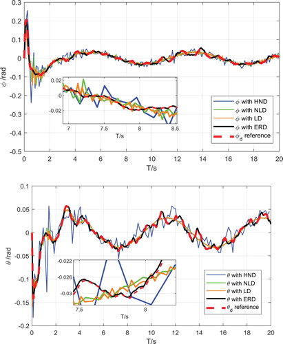
Figure 5. Trajectory tracking with white noise of 0.001 dB intensity.

It can be seen from Figure 6 that, taking the position sub-equation as an example, when the error in the initial stage of control is relatively large, LADRC can well make the control law quickly approach the vicinity of the desired control law interval. The control is gradually stabilized during the middle and rear stages of the control process. To make the control more precise, the NLADRC is used to adjust the error to achieve more accurate and stable control.

Figure 6. White noise 0.001 dB position sub-equipment controller output.

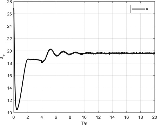
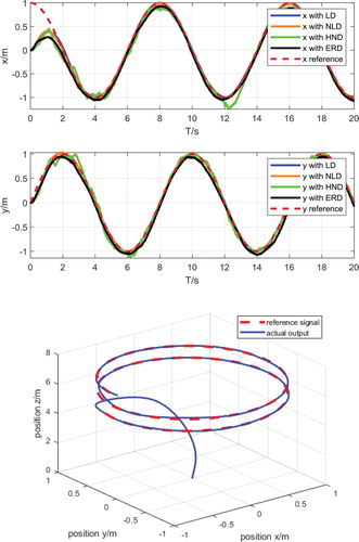
Figure 7 is an attitude tracking diagram after the white noise intensity is increased to 0.01 dB. It can be seen that the attitude and position output curves of the control algorithm remain relatively stable at this time, and there is a phenomenon of chattering at some nodes. Compared to the conventional differentiator, the ERD acts on the pose output of the quadrotor, and it has better performance. Figure 8 is a trajectory tracking diagram after the white noise intensity is increased to 0.01 dB. It can be seen that the smoothness of the flight path of the quadrotor at 0.1 dB is also lower than the lower strength of 0.001 dB.

Figure 7. Attitude tracking and position tracking under white noise of 0.01 dB.

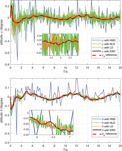
Figure 8. Trajectory tracking with white noise of 0.01 dB intensity.

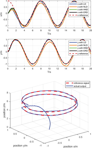
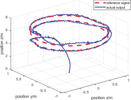
It can be seen from Figure 9 that the flight path of the quadrotor obtained at this time is not smooth, and the smooth performance is not as good as that under low-intensity white noise.

Figure 9. Trajectory tracking with white noise of 0.1 dB intensity.

Conclusion

In this paper, for the anti-disturbance problem of the trajectory tracking control of a quadrotor UAV under white noise disturbance, the quadrotor UAV is controlled by the ADRSC algorithm based on a robust differentiator. Simulation results show that the ERD can extract and filter accurate differential signals in a white noise environment. The ADRSC algorithm can adjust the error in the control process to achieve stable control of the quadrotor UAV. It can improve the anti-disturbance ability and adaptability of the quadrotor UAV to white noise disturbance during the trajectory tracking control process. The algorithm in this paper can achieve stable control of a quadrotor in the white noise range of 0.1 dB. The theoretical basis for the actual control of a quadrotor UAV under white noise is established.

Acknowledgements

We thank LetPub (www.letpub.com) for its linguistic assistance during the preparation of this manuscript.

Disclosure statement

No potential conflict of interest was reported by the author(s).

Additional information

Funding

This work was supported by the National Natural Science Foundation of China [grant numbers 51767022, 51967019].

References

- Bartolini, G., Ferrara, A., Levant, A., & Usai, E. (1999). On second order sliding mode controllers. In K. Young, & Ü Özgüner (Eds.), Variable structure systems, sliding mode and nonlinear control. Lecture notes in control and information sciences (pp. 329–350). Springer.
- Chen, F., Jiang, R., Zhang, K., Jiang, B., & Tao, G. (2016). Robust backstepping sliding-mode control and observer-based fault estimation for a quadrotor UAV. IEEE Transactions on Industrial Electronics, 63(8), 5044–5056. https://doi.org/10.1109/TIE.2016.2552151
- Chen, Z., Sun, M., & Yang, R. (2014). On the stability of linear active disturbance rejection control. Acta Automatica Sinica, 39(5), 574–580. https://doi.org/10.3724/SP.J.1004.2013.00574
- Chen, Z., Wang, C., Li, Y., Zhang, Q., & Sun, M. (2015). Control system design based on integral sliding mode of quadrotor. Journal of System Simulation, 27(9), 2181–2186. doi:10.16182/j.cnki.joss.2015.09.034
- Dolatabadi, S. H., & Yazdanpanah, M. J. (2015). MIMO sliding mode and backstepping control for a quadrotor UAV. In 23rd Iranian Conference on Electrical Engineering (pp. 994–999). IEEE.
- Filippov, A. F. (2013). Differential equations with discontinuous righthand sides: Control systems. Springer Science & Business Media.
- Han, J. (1995). The “extended state observer” of a class of uncertain systems. Control and Decision, 10(1), 85–88. doi:10.13195/j.cd.1995.01.85.hanjq.020
- Han, J. (1998). Auto-disturbances-rejection controller and its applications. Control and Decision, 13(1), 19–23. doi:10.13195/j.cd.1998.01.19.hanjq.004
- Han, J., & Wang, W. (1994). Nonlinear tracking-differentiator. Journal of Systems Science and Mathematical Sciences, 14(2), 177–183.
- Huang, C. (2019). A dynamically event-triggered approach to recursive filtering with censored measurements and parameter uncertainties. Journal of the Franklin Institute, 356(15), 8870–8889. doi:10.1016/j.jfranklin.2019.08.029
- Ibrir, S. (2004). Linear time-derivative trackers. Automatica, 40(3), 397–405. https://doi.org/10.1016/j.automatica.2003.09.020
- Khatoon, S., Shahid, M., Ibraheem, & Chaudhary, H. (2014). Dynamic modeling and stabilization of quadrotor using PID controller. In International Conference on Advances in Computing, Communications and Informatics (ICACCI) (pp. 746–750). IEEE.
- Lee, D., Jin Kim, H., & Sastry, S. (2009). Feedback linearization vs. adaptive sliding mode control for a quadrotor helicopter. International Journal of Control, Automation and Systems, 7(3), 419–428. https://doi.org/10.1007/s12555-009-0311-8
- Levant, A. (2003). Higher-order sliding modes, differentiation and output-feedback control. International Journal of Control, 76(9–10), 924–941. https://doi.org/10.1080/0020717031000099029
- Levant, A. (2005). Homogeneity approach to high-order sliding mode design. Automatica, 41(5), 823–830. https://doi.org/10.1016/j.automatica.2004.11.029
- Levant, A., & Livne, M. (2012). Exact differentiation of signals with unbounded higher derivatives. IEEE Transactions on Automatic Control, 57(4), 1076–1080. https://doi.org/10.1109/TAC.2011.2173424
- Li, J., Qi, X., Xia, Y., & Gao, Z. (2016a). On asymptotic stability for nonlinear ADRC based control system with application to the ball-beam problem. In American Control Conference (ACC) (pp. 4725–4730). IEEE.
- Li, J., Qi, X., Xia, Y., & Gao, Z. (2016b). On linear/nonlinear active disturbance rejection switching control. Acta Automatica Sinica, 42(2), 202–212. https://doi.org/10.16383/j.aas.2016.c150338
- Liu, Y. S., Yang, S. X., & Wang, W. (2015). An active disturbance-rejection flight control method for quad-rotor unmanned aerial vehicles. Control Theory & Applications, 32(10), 1351–1360. https://doi.org/10.7641/CTA.2015.50474
- Shen, B. (2019). Finite-horizon filtering for a class of nonlinear time-delayed systems with an energy harvesting sensor. Automatica, 100, 144–152. doi:10.1016/j.automatica.2018.11.010
- Su, J., Fan, P., & Cai, K. (2011). Attitude control of quadrotor aircraft via nonlinear PID. Journal of Beijing University of Aeronautics and Astronautics, 37(9), 1054–1058. doi:10.13700/j.bh.1001-5965.2011.09.019
- Wang, X., Chen, Z., & Yuan, Z. (2003a). Design and analysis for new discrete tracking-differentiators. Applied Mathematics-A Journal of Chinese Universities, 18(2), 214–222. https://doi.org/10.1007/s11766-003-0027-0
- Wang, X., Chen, Z., & Yuan, Z. (2003b). Nonlinear tracking-differentiator with high speed in whole course. Control Theory and Applications, 20(6), 875–878. https://doi.org/10.3969/j.issn.1000-8152.2003.06.012
- Wang, H., Ye, X., Tian, Y., Zheng, G., & Christov, N. (2016). Model-free–based terminal SMC of quadrotor attitude and position. IEEE Transactions on Aerospace and Electronic Systems, 52(5), 2519–2528. https://doi.org/10.1109/TAES.2016.150303
- Wang, D., Zong, Q., Tian, B., Shao, S., Zhang, X., & Zhao, X. (2018). Neural network disturbance observer-based distributed finite-time formation tracking control for multiple unmanned helicopters. ISA Transactions, 73, 208–226. https://doi.org/10.1016/j.isatra.2017.12.011
- Wu, Y., Sun, J., & Yu, Y. (2016). Trajectory tracking control of a quadrotor UAV under external disturbances based on linear ADRC. In 31st Youth Academic Annual Conference of Chinese Association of Automation (YAC) (pp. 13–18). IEEE.
- Xia, L., Cong, J., Ma, W., Zhao, Y., & Liu, H. (2017). Backstepping sliding mode control of quadrotor attitude system based on immersion and invariance. Journal of Chinese Inertial Technology, 25(5), 695–700. https://doi.org/10.13695/j.cnki.12-1222/o3.2017.05.024