PSO-Markov residual correction method based on Verhulst-Fourier prediction model

Abstract

Macroeconomic predicting is a research hotspot in the field of predicting. The accuracy of predicting often directly affects the rationality of decision-making, especially for defense expenditure predicting. This paper studies the residual correction method of prediction model based on time series. Firstly, based on the grey nonlinear Verhulst prediction model, Fourier series is introduced in this paper to correct the residual sequence once and establish a residual correction model. On this basis, this paper also introduces Markov related concepts, creatively introduces the two-dimensional residual data into Markov state transition matrix, classifies it by K-means clustering analysis, and calculates its parameters by PSO algorithm to realize the secondary accurate correction of residual. Finally, a PSO-Markov residual correction method based on Verhulst-Fourier model is proposed. Tested by examples, this method effectively improves the prediction accuracy of the model, and the prediction is more reliable and accurate.

KEYWORDS:

• Residual correction
• national defense expenditure prediction
• Verhulst-Fourier model
• Markov model
• PSO algorithm

1. Introduction

Prediction refers to a method that calculates the future development trend of the system according to certain methods and laws on the basis of collecting the existing information, so as to understand the development process and results of things in advance (Zeng et al., 2018). As an important part of economic prediction, national defense expenditure prediction is related to the construction and development of the national military strength, it has great practical significance. Prediction based on existing time series has always been an important way to predict complex economic systems. At present, the commonly used economic prediction models include grey prediction model (Niu et al., 2019a; Yan et al., 2019), ARIMA model (Scarpin et al., 2016; Xu et al., 2017), BP neural network model (Wang et al., 2018; Wu et al., 2016; Zhang et al., 2017), SVM regression model (Huang et al., 2019; Yin et al., 2015). However, the economic data under the time series are easily affected by external noise and show complex characteristics such as non-stationarity and randomness (Liu et al., 2017; Zhang & Zou, 2018). So, the data mining technology is usually used to establish a combined predicting model or reasonably correct the predicting residual value of the original predicting model, in order to achieve the purpose of improving the prediction accuracy.

At present, many scholars have done a lot of research on the correction of prediction residual. Huang Yuansheng et al. proposed a load predicting model based on grey Fourier transform residual correction. Firstly, they used the moving average method to improve the original sequence to weaken the influence of outliers, then Fourier transform to improve the general grey prediction model. And by correcting the residual, they eliminated the influence of accidental factors in the sample data (Fang & Huang, 2013). Feng Zengxi et al. established a combination predicting method based on residual correction, and this method is proved for multiple single prediction methods, according to the relative prediction error in a certain period, the combination model can improve the prediction accuracy (Ren & Feng, 2017). According to the multi-period characteristic of the original current carrying sequence, Ma Xiaoming et al. improved the traditional grey model theory, and proposed a method to predict the current carrying capacity of transmission lines by using residual correction basis to compensate the residual value (Fan et al., 2012); Di Yi et al. established a grey Verhulst residual correction model (GVRMM) based on grey theory, to solve the accuracy problem of grey theory in predicting the track of intelligent anti-tank submunitions to ground targets (Gu et al., 2017); Chen Fuji et al. selected multiple index data to establish a multi-factor grey model (MGM(1,m)) for the uncertainty, variability and grey nature of the evolution of network public opinion. They used BP neural network to correct the prediction residual of the multi-factor grey model. So, they constructed a multi-factor grey model based on residual correction (Shi & Chen, 2017). However, due to the single residual correction model and low information utilization, it is impossible to predict the residual values from multiple dimensions. As a result, the residual correction model has great limitations.

In order to solve this problem, this paper proposes a PSO-Markov residual correction method based on Verhulst-Fourier model. Based on the grey Verhulst model, we first use Fourier model to correct the residual once, and introduce Markov model. In view of the problem that the Markov model can only predict the interval of the state set, but cannot accurately obtain the prediction result, K-means clustering analysis and particle swarm algorithm (PSO) are introduced to perform the second correction of the accurate residual. This method integrates Fourier, PSO-Markov, and other residual correction models to scientifically select and use the existing data. The contribution of this model is as follows:

1. On the basis of the Verhulst prediction model, the Fourier series was used to transform the residual data, and the Verhulst-Fourier model was established. The model can extract the implied periodic information in the sample data sequence, make up the fitting error of the data, and modify the prediction residual of Verhulst model, to improve the prediction accuracy. The prediction accuracy of Verhulst-Fourier model is better than Verhulst model.

2. In order to further improve the prediction accuracy, we established a double residual correction model, and used Markov theory and PSO algorithm to carry out the secondary correction of the error fluctuation. Aiming at the limitation and one-sidedness of Markov model, two-dimensional residual state interval division method is used to replace the one-dimensional state interval division method of the traditional Markov model. By replacing the traditional Markov chain subjective division method with K-means cluster analysis, the Markov process is optimized.

3. Since the final prediction of Markov chain is a state interval rather than an accurate value, in order to solve the problems mentioned above, PSO algorithm is introduced to realize the accurate calculation of Markov chain repair value, and the PSO-Markov residual correction method is established.

Aiming at the three points listed above, the PSO-Markov residual error correction method based on Verhulst-Fourier model was established comprehensively, and the military expenditure data were tested by examples. The results showed that the prediction accuracy of the new method was greatly improved compared with that of the traditional method, and a good prediction effect was achieved. It provides an effective method and solution for military expenditure prediction.

2. Verhulst-Fourier residual correction model

2.1. Traditional Verhulst model

Verhulst model is a time series prediction model based on grey system theory, which has unique advantages of small sample modeling for systems with approximate unimodal characteristics of feature sequences (Cui et al., 2015; Xie & Liu, 2015). In particular, the model has good adaptability and predicting effects for ‘S' type original data, and is widely used in economic predicting, railway freight volume predicting, power load predicting, foundation pit settlement predicting, water output predicting, safety situation predicting, and other fields.

Define $X^{(0)}$ as a non-negative raw data sequence (1) $X^{(0)}=(x^{(0)}(1),x^{(0)}(2),\cdot \cdot \cdot ,x^{(0)}(n))$(1) $X^{(1)}$ is the 1-AGO accumulation sequence of $X^{(0)}$ $(x^{(0)}(k)\ge 0,k=1,2,\cdot \cdot \cdot ,n.)$ (2) $\begin{array}{rl}{X}^{(1)}& =(x^{(1)}(1),x^{(1)}(2),\cdot \cdot \cdot ,x^{(1)}(n))\end{array}$(2) (3) $\begin{array}{rl}{x}^{(1)}(k)& =\sum _{i=1}^k{x}^{(0)}(i),k=1,2,\cdot \cdot \cdot ,n.\end{array}$(3) $Z^{(1)}$ is the immediate generation sequence of $X^{(1)}$: (4) $Z^{(1)}=(z^{(1)}(2),z^{(1)}(3),\cdot \cdot \cdot ,z^{(1)}(n))$(4) (5) $z^{(1)}(k)=\theta x^{(1)}(k)+(1-\theta )x^{(1)}(k-1),k=2,3,\cdot \cdot \cdot ,n.$(5) $\theta$ is the adjustment coefficient of the immediate sequence (usually 0.5).

The basic expression formula of Verhulst model: (6) $x^{(0)}(k)+a{z}^{(1)}(k)=b(z^{(1)}(k){)}^2$(6) The parameter column $\hat{a}=[a,b{]}^T$ is obtained according to the least square method: (7) $\hat{a}=(B^{T}B{)}^{-1}{B}^{T}Y$(7) (8) $B=\left(\begin{array}{cc}\begin{array}{c}-z^{(1)}(2)\\ -z^{(1)}(3)\\ ⋮\\ -z^{(1)}(n)\end{array}& \begin{array}{c}{(z^{(1)}(2))}^2\\ {(z^{(1)}(3))}^2\\ ⋮\\ {(z^{(1)}(n))}^2\end{array}\end{array}\right),Y=\left(\begin{array}{c}{x}^{(0)}(2)\\ x^{(0)}(3)\\ ⋮\\ x^{(0)}(n)\end{array}\right)$(8) The whitening equation is: (9) $\frac{d{x}^{(1)}}{dt}+a{x}^{(1)}=b(x^{(1)}{)}^2$(9)

By finding the solution of whitening equation, we can get: (10) $x^{(1)}(t)=\frac{1}{e^{at}[1/x^{(1)}(0)-(b/a)(1-e^{-at})]}$(10) Then the time response formula of Verhulst model is: (11) ${\hat{x}}^{(1)}(k+1)=\frac{a{x}^{(0)}(1)}{b{x}^{(0)}(1)+[a-b{x}^{(0)}(1)]e^{ak}}$(11)

Then restore the data: (12) ${\hat{x}}^{(0)}(k+1)={\hat{x}}^{(1)}(k+1)-{\hat{x}}^{(1)}(k)$(12) In the specific practical application, we often encounter the original data with ‘$S$’ shape. In this case, we can directly regard it as $X^{(1)}$ sequence and directly use Verhulst model, that is using $X^{(1)}$ for accumulation and subtraction, and the accumulation and subtraction 1-IAGO sequence at this time is $X^{(0)}$.

2.2. Verhulst-Fourier model

The traditional Verhulst model is more suitable for ‘S' type time series with saturation state trend. However, in the practical application process, the fitting situation of the original data always deviates from the ideal ‘S' state, thus reducing the prediction accuracy of the model. At the same time, because the internal mechanism of Verhulst model is affected by the selection of initial value $x^{(1)}(1)$ and adjustment coefficient $\theta$ of the immediate generation sequence, the prediction error of the model will also increase. Therefore, on the basis of Verhulst model, Fourier series is introduced to correct the predicted residual value (Niu et al., 2019b; Zachariah et al., 2019).

Fourier series can extract the hidden periodic information in the data sample sequence, and periodic signals or any signals that meet the conditions and can be extended can be expanded into Fourier series (Asnhari et al., 2019). By applying Fourier series to the residual of time series, it has better correction effect. The specific steps are as follows:

Step 1. The traditional Verhulst model is used to fit and predict the original time series, and the fitting and predicted values are output: (13) ${\hat{x}}^{(0)}(k),k=1,2,\cdots ,n+\eta .$(13) The fitting value is the first $n$ terms, the predicted value is the $n+1$ to $n+\eta$ terms, and $\eta$ is the prediction order.

Step 2. Define the residual sequence $E_r$ and calculate: (14) $E_r(k)=x^{(0)}(k)-{\hat{x}}^{(0)}(k),k=1,2,\cdots ,n.$(14)

Step 3. Expand the residual sequence $E_r$ into the form of Fourier series: (15) $E_r(k)=\frac{1}{2}{A}_0+\sum _{i=1}^{\delta }\left[A_i\cos (\frac{2\pi i}{T}\times k)+B_i\sin (\frac{2\pi i}{T}\times k)\right]$(15) In formula (15), $k=1,2,\cdots ,n$; $T=n$ is the interval length; $\delta =[(n-1)/2]-1$ is the lower limit of reasonable expansion degree of finite sequence. $A_0,A_i,B_i$ is approximately estimated by the least square method: (16) $\begin{array}{rl}C& =[\begin{array}{cccccccc}{A}_0& A_1& B_1& A_2& B_2& \cdots & A_n& B_n\end{array}{]}^T.\end{array}$(16) (17) $\begin{array}{rl}C& =(P^{T}P{)}^{-1}{P}^T{E}_r.\end{array}$(17) Among them, the value of $P$ is as follows: (18) $\begin{array}{rl}P& =(\begin{array}{ccc}{\displaystyle \frac{1}{2}}& \cos ({\displaystyle \frac{2\pi \times 1}{T}}\times 1)& \sin ({\displaystyle \frac{2\pi \times 1}{T}}\times 1)\\ {\displaystyle \frac{1}{2}}& \cos ({\displaystyle \frac{2\pi \times 2}{T}}\times 1)& \sin ({\displaystyle \frac{2\pi \times 2}{T}}\times 1)\\ ⋮& ⋮& ⋮\\ {\displaystyle \frac{1}{2}}& \cos ({\displaystyle \frac{2\pi \times n}{T}}\times 1)& \sin ({\displaystyle \frac{2\pi \times n}{T}}\times 1)\end{array}\\ & \begin{array}{ccc}\cdots & \cos ({\displaystyle \frac{2\pi \times 1}{T}}\times \delta )& \sin ({\displaystyle \frac{2\pi \times 1}{T}}\times \delta )\\ \cdots & \cos ({\displaystyle \frac{2\pi \times 2}{T}}\times \delta )& \sin ({\displaystyle \frac{2\pi \times 2}{T}}\times \delta )\\ & ⋮& ⋮\\ \cdots & \cos ({\displaystyle \frac{2\pi \times n}{T}}\times \delta )& \sin ({\displaystyle \frac{2\pi \times n}{T}}\times \delta )\end{array})\end{array}$(18)

Step 4. The Fourier residual correction value and the unknown residual prediction value are calculated by using the known residual value.

The residual value after Fourier series correction is recorded as: (19) ${\hat{E}}_{rF}(k),k=1,2,\cdots ,n+\eta .$(19)

Step 5. The predicted value is restored by using the residual corrected by Fourier series. (20) ${{\hat{x}}_F}^{(0)}(k)={\hat{x}}^{(0)}(k)+{\hat{E}}_{rF}(k),k=1,2,\cdots ,n+\eta .$(20) By modifying the residual value of the original Verhulst model with Fourier series, the fluctuation of the grey prediction model can be reduced, and the adaptability and stability of the prediction model can also be improved.

3. PSO-Markov residual correction method based on Verhulst-Fourier model

3.1. Markov model

Markov chain is a time series without aftereffect, which describes the dynamic change process of random series. It is a method to infer the state of a variable in a certain period in the future according to the initial state probability vector and state probability transition matrix (Chen et al., 2016; Fan & Zhang, 2014). This method requires less historical data, and only needs the recent data of the predicted object to make prediction. It has better error correction effect for data with large random fluctuation. Markov chain is usually combined with other prediction models to achieve the purpose of residual correction. The specific steps are as follows:

Step 1. Division of state interval.

According to the original prediction model, we can calculate its adaptability and prediction values, calculate the error between the fitting value and the actual value, set the state threshold, and divide the error into corresponding state intervals. The division method is usually one-dimensional, the absolute errors or the relative errors between the predicted values and the actual values are used for division.

Step 2. Constructing Markov state transition matrix.

The transition probability of transferring errors from one state to another constitutes a state transition probability matrix. For example, the number of transitions from state $E_i$ to state $E_j$ is $m_{ij}$, and the total number of transitions from state $E_i$ is $M_i$, then the probability of transitions from state $E_i$ to state $E_j$ is $p_{ij}=\frac{m_{ij}}{M_i}$. We construct a state transition probability matrix $P$ (Liu, 2008; Qin, 2013): (21) $P=\left(\begin{array}{cccc}{p}_{11}& p_{12}& \cdots & p_{1n}\\ p_{21}& p_{22}& \cdots & p_{2n}\\ ⋮& ⋮& \ddots & ⋮\\ p_{n1}& p_{n2}& \cdots & p_{nn}\end{array}\right)$(21) If the current state is predicted backward $\eta$ times, the transition probability matrix becomes $P^{\eta }$ accordingly.

Step 3. Error correction

After the state transition probability matrix is determined, the next state that is most likely to occur can be predicted according to the current base state. According to the range interval of the state, the error of this state can be reasonably estimated, and its error is $\Delta \epsilon (t+\eta )$, $t$ is the current state time, and $\eta$ is the prediction order.

Step 4. Output the corrected predicted value (22) ${{\hat{x}}_M}^{(0)}(t+\eta )={{\hat{x}}_{}}^{(0)}(t+\eta )+\Delta \epsilon (t+\eta )$(22)

Note: In practical application, due to the need to continuously consider the disturbance factors that enter the system one after another with the passage of time and highlight the role of new data, the old information that is old or of little value is often deleted from the system in the form of sliding windows (Wu et al., 2013). The detailed operations are as follows: Through calculation, after adding a set of data, the earliest set of data is eliminated, historical data is diluted, new information entering the system is put into the residual sequence at any time, and update calculation is continuously carried out. This is also a form of residual fluctuation correction commonly used in Markov chains.

3.2. PSO-Markov residual correction model

The traditional Markov chain has good effect in error fluctuation correction, but there are also some problems. First of all, the traditional Markov chain has great subjectivity in the division of state intervals. Most of them are established subjectively according to the actual errors or adopt a simple equidistant division method to select state thresholds, which is easy to cause individual data with large errors to expand the range of state intervals, while most data have small ranges. Secondly, most of them adopt one-dimensional state interval division method, which also limits the model to some extent, resulting in the limitation and one-sidedness of its state division. Thirdly, Markov chain finally predicts a state interval, and its accurate correction value is usually determined by averaging. If the state interval range is too large, the error will easily increase. In order to solve the above problems, this paper introduces K-means clustering analysis and PSO algorithm based on two-dimensional data to improve Markov chain.

PSO algorithm is a population set intelligent optimization algorithm proposed by Kennedy and Eberhart in 1995 according to the social behaviour of birds. In PSO algorithm, the potential solution of the optimization problem is equivalent to solving a particle in n-dimensional search space that meets the constraint conditions and particle motion trend. PSO algorithm first generates several randomly distributed search particles, and these search particles move at a certain speed in the search space, which depends on their inertia, optimal position, and the optimal position of the population (Huang & He, 2018; Qiao et al., 2017).

Considering the current intelligent algorithms comprehensively, the commonly used intelligent algorithms at present include genetic algorithm (GA), simulated annealing algorithm (SA), BP neural network and PSO particle swarm optimization algorithm. GA and PSO algorithm of individual difference lies in: The individuals of GA are chromosomes, characterized by genes; but the individuals of PSO are particles, characterized by position, velocity, and neighbourhood group. Compared with GA genetic algorithm, PSO algorithm has the property of ‘memory’ of particles. They learn by ‘self’ and learn from ‘others’, and the whole particle swarm can preserve such memory, while GA algorithm gene has no memory ability. In addition, compared with GA, PSO does not require coding and has no crossover and mutation operation, making it easier to operate. Compared with SA, PSO algorithm requires fewer parameters to be adjusted, and its implementation is relatively simple and efficient. Moreover, the algorithm has good robustness, stability, and easy convergence to obtain the optimal solution. Compared with BP algorithm, PSO algorithm does not strictly abide by the principle of error gradient descent as BP algorithm does. Through self-renewal of particles, PSO enables its ‘descendants’ to inherit more information from their predecessors in a targeted way to find the optimal solution in a shorter period of time. When faced with local minima, the error gradient is usually zero, BP algorithm cannot distinguish the minima, while PSO can finally achieve a global optimization effect by updating the current best position of each particle and the best position of the whole population. In summary, the most important feature of PSO algorithm is that it can find the global optimal solution of the problem to be solved with high probability. It is simple and easy to realize, has fast convergence speed and good robustness, and is more suitable for optimizing the parameters in The Markov model, to improve the Markov chain.

Therefore, in this paper, the accurate calculation of Markov chain correction value is realized by using the characteristics of simple implementation, few parameter settings and fast convergence speed of the PSO algorithm. The detailed steps of PSO-Markov are as follows:

Step 1. Firstly, we use Verhulst-Fourier model to make preliminary prediction, and calculate the absolute error and relative error of the model.

Step 2. Two-dimensional data processing

We process the absolute error and the relative error to make the data fluctuation within a reasonable range, control the amplitude difference of the data itself, and avoid causing the data weight of a certain dimension to be too large.

Step 3. State interval division

We use K-means clustering analysis algorithm to classify two-dimensional data. K-means aims at dividing the data (Qiu et al., 2014). The realization of this goal is to divide the data according to the input parameter k and divide it into k clusters. The biggest characteristic of this classification method is simplicity and convenience, and the obtained effect is also good. Then, we need to divide the classified data into specific state intervals.

Step 4. Constructing Markov state transition matrix.

According to formula (13), we construct Markov state transition matrix for two-dimensional data.

Step 5. Accurate calculation of error correction value.

We use Markov state transition matrix to predict the most likely next state according to the current base state, and combine PSO algorithm to accurately calculate the error correction value. The update formulas of velocity, position, and inertia weight of each particle in PSO algorithm are as follows (Liu & Yang, 2011): (Assuming that N particles form a community in D-dimensional target search space) (23) $\{\begin{array}{l}{\displaystyle x_{i,j}(t+1)=x_{i,j}(t)+v_{i,j}(t+1),i=1\cdots d}\\ {\displaystyle v_{i,j}(t+1)=w\cdot v_{i,j}(t)+c_1{r}_1[p_{i,j}-x_{i,j}(t)]}\\ +c_2{r}_2[p_{g,j}-x_{i,j}(t)]\\ {\displaystyle w=w_{max}-\frac{w_{max}-w_{min}}{ite{r}_{max}}\times K}\end{array}$(23) In formula (23), $v_{i,j}(t)$ is the $d$ dimensional flight velocity of particle $i$ at $t$ iterations, $d=1,2,\cdots ,D$; $p_{i,j}$ and $p_{g,j}$ are the $d$ dimensional local optima of particle $i$ and the $d$ dimensional global optima of the whole particle swarm; $x_{i,j}(t)$ is the $d$ dimensional position of particle $i$ at $t$ iterations; $r_1$ and $r_2$ are random numbers between $(0,1)$, which are used to maintain population diversity; $c_1$ and $c_2$ are learning factors; $w$ is the inertia weight, $w_{max}$ is the maximum inertia weight, $w_{min}$ is the minimum inertia weight, and $ite{r}_{max}$ is the maximum number of iterations.

We can obtain the characterization error that defaults to this state by averaging the classified errors of each dimension. Then, we predict the next state that is most likely to occur through Markov state transition matrix. We can obtain the two-dimensional characterization error of the state, and restore the processed data according to the idea of step 2. Finally, we can accurately calculate the residual correction value through PSO algorithm to obtain the residual value corrected by PSO-Markov, among them, $t$ is the current state time and $\eta$ is the prediction order.

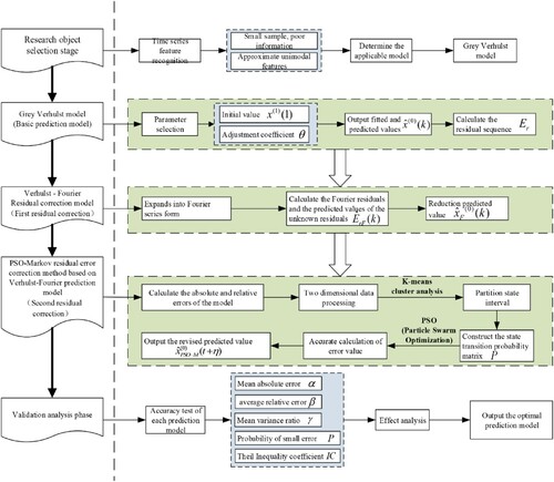
Step 6. Output the corrected predicted value. (24) ${{\hat{x}}^{(0)}}_{PSO-M}(t+\eta )$(24) According to the above ideas, the general idea diagram of PSO-Markov residual error correction method based on Verhulst-Fourier model is illustrated in Figure 1.

Figure 1. Idea diagram of PSO-Markov residual correction method based on Verhulst-Fourier model.

4. Instance validation

4.1. Data source

In this paper, we choose India’s defense expenditure data from 1992 to 2017 (Table 1) to verify the prediction accuracy of the residual correction method. The group of data shows an overall upward trend (Figure 2), but there is also a decline in local data. We use India’s defense expenditure data from 1992 to 2012 as the original time series, and use India’s defense expenditure data from 2013 to 2017 as the test data of PSO-Markov Residual Correction Method Based on Verhulst-Fourier Model.

Figure 2. India’s defense expenditure trend chart.

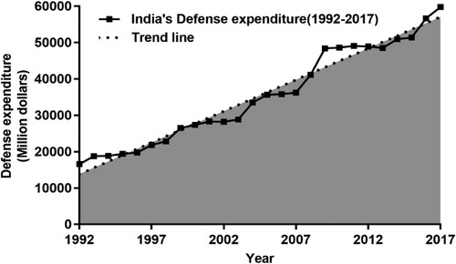
Table 1. India’s defense expenditure from 1992 to 2017 (Million USD).

Year	Defense expenditure (Million USD)	Year	Defense expenditure (Million USD)	Year	Defense expenditure (Million USD)
1992	16592.26	2001	28291.25	2010	48600.22
1993	18740.27	2002	28203.69	2011	49071.05
1994	18823.90	2003	28833.48	2012	48896.45
1995	19388.12	2004	33492.84	2013	48536.29
1996	19739.67	2005	35643.71	2014	50908.91
1997	21851.06	2006	35814.37	2015	51392.59
1998	22797.96	2007	36247.95	2016	56637.62
1999	26494.60	2008	41113.38	2017	59757.11
2000	27339.12	2009	48406.73

Note: All data are from the official website of the Stockholm International Peace Research Institute (SPIRI), with 2016 US dollars as the benchmark currency.

4.2. Model accuracy test index

The accuracy test methods of the prediction model include relative error, absolute error, posterior error method and residual test method (Boussetta et al., 2013; Ren et al., 2011), and the specific accuracy test indexes include absolute error, relative error, correlation degree, standard deviation ratio, small error probability, Theil inequality coefficient, etc. The formulas are listed as follows:

1. Absolute error $\alpha$ (25) $\alpha =\frac{1}{n}\sum _{j=1}^n|e_j|=\frac{1}{n}\sum _{j=1}^n\left|\widehat{y_j}-y_j\right|$(25)

The smaller the $\alpha$, the higher the prediction accuracy.

1. Relative error $\beta$ (26) $\beta =\frac{1}{n}\sum _{j=1}^n\left|\frac{\widehat{y_j}-y_j}{y_j}\right|$(26)

2. Standard deviation ratio $\gamma$ (27) $\gamma =S_2/S_1$(27)

In formula (27), $S_1$ is the standard deviation of the original data; $S_2$ is the standard deviation of the residual.

1. Small error probability $P$ (28) $P=P\{|e(i)-\stackrel{-}{e}|<0.6745S_1\}$(28)

In formula (28), $\stackrel{-}{e}$ is the mean value of residual.

Note: The small error probability P is subject to the standard normal distribution, and the error probability should fall within the range of 25% to 75%. According to the normal distribution table, the corresponding values of 25% and 75% are −0.6745 and +0.6745 respectively (Table 2).

1. Theil inequality coefficient $IC$ (29) $IC=\frac{\sqrt{\frac{1}{n}\sum _{j=1}^n{(\widehat{y_j}-y_j)}^2}}{\sqrt{\frac{1}{n}\sum _{j=1}^n{\widehat{y_j}}^2}+\sqrt{\frac{1}{n}\sum _{j=1}^n{y_j}^2}}$(29)

Table 2. Reference standards for $IC$ evaluation indicators.

Accuracy grade	Relative error	Standard deviation ratio	Small error probability p
Level I (Great)	0.01	0.35	0.95
Level II (Qualified)	0.05	0.50	0.80
Level III (Poor)	0.10	0.65	0.70
Level IV (Unqualified)	0.20	0.80	0.60

4.3. Prediction and analysis of defense expenditure

We substituted India’s Defense expenditure data from 1992 to 2012 into the traditional Verhulst model (hereinafter referred to as model I) to make a preliminary predict and obtain its predict value. Then, we use Verhulst-Fourier first residual error correction model (hereinafter referred to as model II) to expand the residual into Fourier series form, and set $\delta =8$, to correct the residual. Then we use the corrected residual to predict the residual value from 2013 to 2017 and return to the predicted value. The fitting values of the two models are shown in Table 3. Two models were used to predict the predicted value, as shown in Table 4. The accuracy of the two models is compared by the evaluation indexes established above, as shown in Table 5.

Table 3. Fitting values of model I and model II.

		Model I			Model II
Year	Actual value (Millions USD)	Fitting value	Absolute error	Relative error	Fitting value	Fourier corrected absolute residual	Fourier corrected relative residual
1992	16592	16592.00	0.00	0.00%	16591.69	0.57	0.00%
1993	18740	17841.33	898.67	4.80%	19032.75	292.49	1.56%
1994	18824	19156.81	332.81	1.77%	18599.38	224.52	1.19%
1995	19388	20537.82	1149.82	5.93%	19511.12	122.99	0.63%
1996	19740	21983.08	2243.08	11.36%	19575.48	164.19	0.83%
1997	21851	23490.63	1639.63	7.50%	22272.44	421.38	1.93%
1998	22798	25057.78	2259.78	9.91%	22080.10	717.86	3.15%
1999	26495	26681.11	186.11	0.70%	27230.16	735.56	2.78%
2000	27339	28356.43	1017.43	3.72%	26949.00	390.12	1.43%
2001	28291	30078.86	1787.86	6.32%	28238.66	52.59	0.19%
2002	28204	31842.80	3638.80	12.90%	28532.83	329.14	1.17%
2003	28833	33642.05	4809.05	16.68%	28468.60	364.88	1.27%
2004	33493	35469.83	1976.83	5.90%	33804.71	311.87	0.93%
2005	35644	37318.90	1674.90	4.70%	35330.97	312.74	0.88%
2006	35814	39181.69	3367.69	9.40%	36101.84	287.47	0.80%
2007	36248	41050.38	4802.38	13.25%	36209.00	38.94	0.11%
2008	41113	42917.05	1804.05	4.39%	40659.71	453.67	1.10%
2009	48407	44773.83	3633.17	7.50%	49335.65	928.92	1.92%
2010	48600	46612.99	1987.01	4.09%	47718.91	881.31	1.81%
2011	49071	48427.13	643.87	1.31%	49310.04	238.99	0.49%
2012	48896	50209.23	1313.23	2.68%	49466.10	569.64	1.17%
Average absolute error			1960.29			373.33
Average relative error				6.42%			1.21%

Table 4. Predicted values of model I and model II.

		Model I			Model II
Year	Actual value (Millions USD)	Predicted values	Absolute error	Relative error	Predicted values	Absolute Error	Relative error
2013	48536.29	53651.91	5115.91	10.54%	47362.54	1173.74	2.42%
2014	50908.91	55301.35	4392.35	8.63%	52028.67	1119.76	2.20%
2015	51392.59	56896.57	5503.57	10.71%	50723.81	668.78	1.30%
2016	56637.62	58433.78	1795.78	3.17%	56974.93	337.31	0.60%
2017	59757.11	59909.93	152.93	0.26%	59488.76	268.34	0.45%

Table 5. Comparison of prediction accuracy between model I and model II.

	Average absolute error $\alpha$	Average relative error $\beta$	Standard deviation ratio $\gamma$	Small error probability $P$	Theil inequality coefficient $IC$
Model I	3392.11	6.66%	0.5033	0.80	0.0359
Model II	713.58	1.39%	0.1936	1.00	0.0076

Through comparison, we can conclude that the five model accuracy test indexes of model II are better than model I. In order to further improve the prediction accuracy, we introduce PSO-Markov method to correct the residual value further accurately. Firstly, we process the data of the two-dimensional residual value generated by model II fitting, and take the logarithm with the bottom of 10 (plus and minus signs are reserved) as C1 for its absolute error. We multiply the relative error by 1000 times square it (keep the plus and minus signs) and denote it as C2. Then, we use K-means clustering algorithm to divide the processed two-dimensional residual data and obtain its corresponding state, which is divided into three states according to the number of data: E1, E2 and E3, as shown in Table 6. The processed two-dimensional residual data are shown in Figure 3, and the k-means clustering analysis scatter diagram is shown in Figure 4.

Figure 3. Two-dimensional residual data graph.

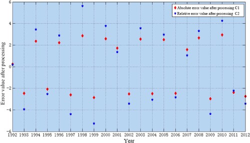
Figure 4. K-means cluster analysis scatter diagram.

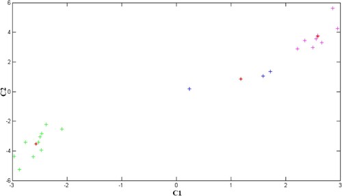
Table 6. State partition of two-dimensional residual data after processing.

Year	C1	C2	State
1992	0.24	0.19	E2
1993	−2.47	−3.95	E3
1994	2.35	3.45	E1
1995	−2.09	−2.52	E3
1996	2.22	2.88	E1
1997	−2.62	−4.39	E3
1998	2.86	5.61	E1
1999	−2.87	−5.27	E3
2000	2.59	3.78	E1
2001	1.72	1.36	E2
2002	−2.52	−3.42	E3
2003	2.56	3.56	E1
2004	−2.49	−3.05	E3
2005	2.50	2.96	E1
2006	−2.46	−2.83	E3
2007	1.59	1.04	E2
2008	2.66	3.32	E1
2009	−2.97	−4.38	E3
2010	2.95	4.26	E1
2011	−2.38	−2.21	E3
2012	−2.76	−3.41	E3

The mean values of C1 and C2 in the three state intervals (E1, E2 and E3) are obtained in Table 7.

Table 7. Mean value of two-dimensional residual data in state interval.

State interval	C1 mean value	C2 mean value
E1	2.58	3.73
E2	1.18	0.86
E3	−2.56	−3.54

Since the state transition is random, the probability must be used to describe the possibility of the state transition, that is, the state transition probability. According to the relevant probability calculation formulas in 2.1, we can construct a state transition probability matrix. According to the above division (Table 6), we can easily obtain Markov’s first-order state transition matrix $P_{}$.

According to Table 6, we can see that there are 21 groups of 2d residual data after processing. Since the last group of transfer states is unknown, there are 20 state transfer processes. The E1 state occurs 8 times, including 0 transitions to E1 state, 1 transition to E2 state, and 7 transitions to E3 state. The E2 state occurs 3 times, including 1 transition to E1 state, 0 transition to E2 state, and 2 transitions to E3 state. The E3 state occurs 9 times (because the last set of states is unknown, the last set of states is abandoned), including 7 transitions to E1 state, 1 transition to E2 state, and 1 transition to E3 state. According to the contents in the 2.1 Markov Model, we can calculate the state transition probability $p_{ij}$ separately. $\begin{array}{rl}{p}_{11}& =1/8,p_{12}=0,p_{13}=7/8;\end{array}$ $\begin{array}{rl}{p}_{21}& =1/3,p_{22}=0,p_{23}=2/3;\end{array}$ $\begin{array}{rl}{p}_{31}& =7/9,p_{32}=1/9,p_{33}=1/9.\end{array}$

The state transition probability matrix $P_{}$ can be obtained as follows: $P_{}=\left(\begin{array}{ccc}0& 1/8& 7/8\\ 1/3& 0& 2/3\\ 7/9& 1/9& 1/9\end{array}\right)$According to the first order state transition probability matrix $P$, we can obtain $\eta$ order state transition matrix $P^{\eta }$.

By using the mean value of the state in Table 7 as the two-dimensional residual characterization value of the state, restoring the data of the two-dimensional residual characterization value, and then correcting the residual using particle swarm optimization algorithm, we can obtain the final predicted value ${{\hat{x}}^{(0)}}_{PSO-M}(t+\eta )$.

The fitness function is: (30) $f=\sum _{k=n+1}^{n+\eta }\left[q_1\cdot [{{\hat{x}}_F}^{(0)}(k)\pm {10}^{C_1}]+q_2\cdot \frac{{{\hat{x}}_F}^{(0)}(k)}{1\pm \frac{C_2}{1000}}\right]$(30) $q_1,q_2$ are weight values.

Through calculation, we can get $q_1$ = 0.172, $q_2$ = 0.827, and get the final prediction value of PSO-Markov residual correction method based on Verhulst-Fourier prediction model (model III), as shown in Table 8 and Figure 5.

Figure 5. Actual values and predicted values of models I, II and III.

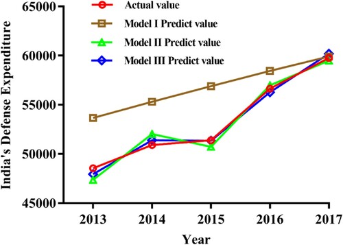
Table 8. Final predicted values of PSO-Markov residual correction method based on Verhulst-Fourier model.

		Model III
Year	Actual value (Millions USD)	Predicted values	Absolute error	Relative error
2013	48536.29	47941.20	595.09	1.23%
2014	50908.91	51390.14	481.23	0.95%
2015	51392.59	51338.89	53.69	0.10%
2016	56637.62	56281.63	355.99	0.63%
2017	59757.11	60198.84	441.73	0.74%

The prediction accuracies of model I, II and III were compared, as shown in Table 9. The absolute errors of predicted values in model I, II and III were compared, as shown in Figure 6(a); and the relative errors of predicted values in model I, II and III were compared, as shown in Figure 6(b).

Figure 6. Comparison of predictive value errors in model I, model II and model III.

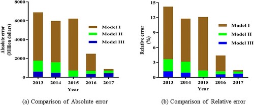
Table 9. Prediction accuracy of model III.

	Average absolute error $\alpha$	Average relative error $\beta$	Standard deviation ratio $\gamma$	Small error probability $P$	Theil inequality coefficient $IC$
Model I	3392.11	6.66%	0.5033	0.80	0.0359
Model II	713.58	1.39%	0.1936	1.00	0.0076
Model III	385.55	0.73%	0.0444	1.00	0.0040

Through the comparison and analysis of three models mentioned above, we can see that the PSO-Markov residual correction method based on Verhulst-Fourier model (Model III) is obviously better than model I and model II in five accuracy test indexes. So, the predicted value of model III is closer to the actual value and the prediction effect is optimal.

5. Conclusion

This paper proposes a PSO-Markov residual correction method based on Verhulst-Fourier model. First of all, Fourier series was used to extract the implicit periodic information in the sample data sequence and it can compensate the fitting error of the data, so the prediction residual error of Verhulst model was preliminarily corrected. Secondly, two-dimensional data processing and k-means algorithm are used to optimize the Markov state interval division, which solves the problem of single data dimension state interval division and strong subjectivity in the traditional Markov model. Thirdly, PSO algorithm can effectively model the prediction residual value for precise correction, solve the problem of interval fuzzy Markov state set accurate correction residual value. In general, the new method greatly improves the prediction accuracy and provides a new idea for the correction direction of the residual error of the prediction model. Also, this method can predict military expenditure with higher accuracy, less fluctuation of error, better stability, and reliability, and effectively support and promote the research of military expenditure forecast.

Disclosure statement

No potential conflict of interest was reported by the author(s).

Additional information

Funding

This work was supported by China Postdoctoral Science Foundation [grant number 2017M623417].

References

- Asnhari, S. F., Gunawan, P. H., & Rusmawati, Y. (2019). Predicting staple food materials price using multivariables factors (Regression and Fourier models with ARIMA). 2019 7th International Conference on Information and Communication Technology (ICoICT).
- Boussetta, S., Balsamo, G., Beljaars, A., Kral, T., & Jarlan, L. (2013). Impact of a satellite-derived leaf area index monthly climatology in a global numerical weather prediction model. International Journal of Remote Sensing, 34(9-10), 3520–3542. https://doi.org/https://doi.org/10.1080/01431161.2012.716543
- Chen, H. L., Leng, H., & Li, X. R. (2016). A modified Fourier-Markov model for medium and long-term electricity predicting. Journal of Hunan University (Natural Science Edition), 43(10), 62–69.
- Cui, J., Zhao, L., & Liu, S. F. (2015). Parameter characteristics of a new grey Verhulst prediction mode. Control and Decision, 30(11), 2093–2096.
- Fan, C. J., Hu, T. Q., & Ma, X. M. (2012). Predict and analysis of transmission line current carrying capacity based on periodic residual modified grey model. Power System Protection and Control, 40(19), 19–23.
- Fan, K. W., & Zhang, S. P. (2014). Dam deformation prediction based on adaptive MGM(1, n)-Markov chain model. South-to-North Water Transfer and Water Conservancy Science and Technology, 12(1), 145–148.
- Fang, W., & Huang, Y. S. (2013). Power load predicting model based on grey Fourier transform residual correction. Power Automation Equipment, 33(9), 105–107. 112.
- Gu, X. H., Long, F., & Di, Y. (2017). Target track prediction method based on grey residual correction theory. Journal of Military Engineering, 38(3), 454–459.
- Huang, J., & He, Z. G. (2018). Predict of railway freight volume based on FPSO grey Verhulst model. Journal of Railways, 40(8), 1–8.
- Huang, J., Liang, Y., Bian, H., & Wang, X. (2019). Using cluster analysis and least square support vector machine to predicting power demand for the next-day. IEEE Access, 7, 82681–82692. https://doi.org/https://doi.org/10.1109/ACCESS.2019.2922777
- Liu, C. H. (2008). Stochastic processes. Huazhong University of Science and Technology Press, 2008, 42–43.
- Liu, B. P., Huang, D., & Zhang, K. (2017). Small sample nonlinear residual grey Verhulst quantitative combination predicting model based on EGA algorithm. Systems Engineering Theory and Practice, 37(10), 152–161.
- Liu, Y. Q., & Yang, Z. L. (2011). Short-term wind power prediction using particle swarm optimization algorithm. Power Grid Technology, 35(5), 159–164.
- Niu, T., Zhang, L., Wei, S. J., Li, B., & Zhang, B. (2019a). Initial value modified Verhulst model based on reverse prediction. Mathematical Practice and Understanding, 49(18), 161–167.
- Niu, T., Zhang, L., Wei, S., & Zhang, B. (2019b). Study on a combined prediction method based on BP neural network and improved Verhulst model. Systems Science & Control Engineering, 7(3), 36–42. https://doi.org/https://doi.org/10.1080/21642583.2019.1650672
- Qiao, H. Q., Guo, Z. Q., & Liu, C. (2017). Inversion of shale pore structure and shear wave velocity prediction based on particle swarm optimization. Progress in Geophysics, 32(2), 689–695.
- Qin, S. (2013). Weighted moving average-Markov prediction model and its application. Journal of Water Resources and Water Engineering, 24(1), 185–188.
- Qiu, Q., Zhang, Q., & Guo, K. (2014). Grey Kmeans algorithm and its application to the analysis of regional competitive ability. Information technology & artificial intelligence conference, IEEE.
- Ren, Q. C., & Feng, Z. X. (2017). Prediction method based on dynamic combined residual correction. Systems Engineering Theory and Practice, 37(7), 1884–1891.
- Ren, Y. T., Wang, F. L., & Zhang, X. (2011). Prediction of annual precipitation based on improved grey Markov model. Mathematical Practice and Understanding, 41(11), 51–57.
- Scarpin, C. T., Luiz, A. T. J., & Pereria, E. N. (2016). Time series predicting by using a neural ARIMA model based on wavelet decomposition. Independent Journal of Management & Production, 7(1), 252–270.
- Shi, R., & Chen, F. J. (2017). Research on Internet public opinion predict based on multi-factor grey model with residual correction. Information Science, 35(9), 131–135.
- Wang, J. J., Hu, S. G., Zhan, X. T., Luo, Q., Yu, Q., Liu, Zhen, Chen, T. P., Yin, Y., Hosaka, S., Liu, Y. (2018). Predicting house price with a memristor-based artificial neural network. IEEE Access, 6, 16523–16528. https://doi.org/https://doi.org/10.1109/ACCESS.2018.2814065
- Wu, Q. Q., Yuan, H. Z., & Rui, H. T. (2013). Predict method of highway passenger volume based on exponential smoothing method and Markov model. Journal of Transportation Engineering, 13(4), 87–93.
- Wu, Y. P., Zhao, S. P., & Zhang, Y. P. (2016). Prediction of insulator leakage current based on genetic BP neural network. Journal of Railways, 38(5), 46–52.
- Xie, N., & Liu, S. (2015). Interval grey number sequence prediction by using non-homogenous exponential discrete grey forecasting model. Journal of Systems Engineering and Electronics, 26(1), 96–102. https://doi.org/https://doi.org/10.1109/JSEE.2015.00013
- Xu, D.-W., Wang, Y.-D., Jia, L.-M., Qin, Y., Dong, H.-H. (2017). Real-time road traffic state prediction based on Arima and Kalman filter. Frontiers of Information Technology & Electronic Engineering, 18(2), 287–302. https://doi.org/https://doi.org/10.1631/FITEE.1500381
- Yan, Q. S., Zhu, S. Y., & Chen, D. Y. (2019). Grey prediction of spatial alignment of arch ribs of special-shaped arch bridges based on MGM (1, n) model. Journal of South China University of Technology (Natural Science Edition), 47, 120–127.
- Yin, G. L., Zhang, G. R., & Huang, F. M. (2015). Prediction of landslide groundwater level by multivariate PSO-SVM model. Journal of Zhejiang University (Engineering Edition), 49(6), 1193–1200.
- Zachariah, C., Humza, S., & Dhireesha, K. (2019). Analysis of wide and deep echo state networks for multiscale spatiotemporal time series predicting. Proc. of the 7th Annual Neuro-inspired Computational Elements Workshop.
- Zeng, B., Yin, X. Y., & Meng, W. (2018). Practical grey prediction modeling method and its MATLAB implementation. Science Press.
- Zhang, S. Q., Zhang, C., & Jiang, C. L. (2017). Modeling and prediction of MODIS leaf area index time series based on SARIMA-BP neural network combination method. Spectroscopy and Spectral Analysis, 37(1), 189–193.
- Zhang, R., & Zou, Q. (2018). Time series prediction and anomaly detection of light curve using lstm neural network. Journal of Physics: Conference Series, 1061, 012012. https://doi.org/https://doi.org/10.1088/1742-6596/1061/1/012012