Finite-time asynchronous sliding mode control for Markov jump systems with actuator saturation

Abstract

This paper deals with the finite-time asynchronous sliding mode control for Markov jump systems subject to actuator saturation. The hidden Markov model is adopted to describe the modal information exchange between the system and the designed controller. A sufficient condition is established by employing the Lyapunov stability theorem, which guarantees the stochastic finite-time boundedness of sliding mode. In order to mitigate the effects of actuator saturation and chattering, an adaptive sliding mode controller is designed based on the auxiliary saturation compensation system. Subsequently, the reachability of sliding mode motion is analysed. The controller gain matrix is obtained by solving the minimization problem. Finally, a simulation example is used to demonstrate that the proposed control method can effectively restrain the disturbance and compensate saturation.

Keywords:

• Sliding mode control
• Markov jump systems
• actuator saturation
• hidden Markov model
• stochastic finite-time boundedness

1. Introduction

Sliding mode control is a kind of control method with discontinuous control behaviour. Its basic principle is to design a sliding mode controller, such that the trajectory of system starting from any initial state can be driven to the predetermined sliding surface in finite-time and keep moving on it without being affected by other external factors. Different from the continuous sliding mode control, the discrete sliding mode control is quasi sliding mode motion, i.e. the system states are only forced to enter the small bounded neighbourhood near the sliding surface instead of staying on the sliding surface (Janardhanan & Bandyopadhyay, 2006). The sliding mode can be automatically switched according to the control requirements, and it is insensitive to matching uncertainty and external disturbances. Therefore, sliding mode control has the advantages of good transient performance, fast response speed, strong robustness and simple design ideas, which has been widely concerned (Ding et al., 2014; Du et al., 2019; Hu et al., 2012).

In industrial applications, the systems will always switch between different states when it faces machine failure, sudden change of environment (Ma & Liu, 2020). Hence, the single and deterministic model can not solve this type of control problem. But the Markov jump systems have great advantages in dealing with the problem (Liu et al., 2018). The Markov jump systems are a kind of sensitive stochastic systems, which can reflect the change of system structure and parameters through the jump of Markov chain. And the Markov jump systems are widely used in power systems, networked control systems and aircraft flight systems. In recent years, the researches on the stability, stabilization, filter and fault diagnosis of the Markov jump systems have achieved fruitful results (Song, H. et al., 2017; Wu & Mu, 2019; Zha et al., 2017; Zhan et al., 2010). For example, the event-triggered $H_{\mathrm{\infty }}$ control problem has been studied for the networked Markov jump systems in Zha et al. (2017), where different modes correspond to different trigger thresholds. The event-triggered control problem has been investigated for a class of semi-Markov jump systems in Wu and Mu (2019), and the stochastic stability has been analysed for the closed-loop stochastic semi-Markov time delay systems with the help of stochastic system theory. In Song, H. et al. (2017), the sliding mode control problem has been discussed for the discrete systems with Markov packet dropout. The influence of packet dropout on stability has been solved by using Markov jump systems. In Zhan et al. (2010), the static output feedback control has been studied for linear Markov jump systems, and an augmentation method has been proposed which overcomes the problem that the rank of the system matrix often be constrained when dealing with the output feedback control.

In the networked control systems, it is very popular to describe asynchronous phenomenon by introducing the hidden Markov model. The problem of asynchronous stochastic stabilization has been explored for Markov jump systems in Guan et al. (2019), and the necessary and sufficient conditions of asynchronous stochastic stability have been obtained. The hidden Markov model is a statistical model used in many real-world applications. It is a doubly stochastic finite model which calculates probability distribution over an infinite number of possible sequences. It is used for studying the observed items from a discrete-time series. States have assigned transition probabilities, and every state emits symbol according to the emission probability of the state. By adopting the hidden Markov model with partially acceptable modal detection probability to characterize the asynchronous phenomenon, the asynchronous sliding mode control has been studied for a class of uncertain Markov jump systems with time-delay and disturbance in Song, Niu et al. (2018), where the asynchronous sliding mode control law has been designed. In Song, J. et al. (2017), the asynchronous control has been discussed for time-varying Markov jump systems, after utilizing hidden Markov model to deal with the asynchronous phenomenon between the system mode and the controller mode, the sufficient condition of finite-time stochastic boundedness has been obtained which satisfies $H_{\mathrm{\infty }}$ performance. In the research of networked systems, in order to save network resources and reduce data conflicts, the network communication protocol and the signal quantization technology are usually applied (Liu et al., 2014). Many research results show that the protocols and the quantification have played effective roles in coordinating network resources and reducing network burdens, and they have also played an important role in sliding mode control research. By constructing the Lyapunov function based on scheduling signals, the sliding mode control has been analysed for uncertain control systems with Round-Robin protocol in Song, Wang et al. (2018), where a novel output feedback sliding mode controller has been designed. A new event-triggered sliding mode control method has been proposed for networked switching systems in Shang and Zong (2020), besides, a sliding mode controller has been designed which relies on scheduling signals under Round-Robin protocol. The quantitative feedback sliding mode control has been proposed for linear uncertain systems in Zheng et al. (2014), and a static adjustment strategy has been designed for quantitative parameters to eliminate the influence of uncertainty. On the basis of Zheng et al. (2014), by introducing a dynamic uniform quantizer and combing the quantization error with the system output, the $H_{\mathrm{\infty }}$ sliding mode controller has been constructed for the time-delay Markov jump systems in Zhang and Shen (2019).

In addition, the nonlinear constraints and the external disturbances are unavoidable in networked control systems (Han et al., 2020; Jenabzadeh & Safarinejadian, 2018). There are challenging subjects to study the influence of different nonlinear constraints and various external disturbances on the system stability by using the sliding mode control method. Recently, the design problems of output feedback sliding mode controller and dynamic compensator have been studied for the systems with sector bounded actuator amplitude and rate saturation nonlinear constraint in Kapila and Haddad (2000), which has ensured the asymptotic stability of the closed-loop system. The asynchronous control problem has been researched for the Markov jump systems in Yang and Lin (2019), and the closed-loop system satisfies the performance index in a given finite-horizon. In order to compensate actuator saturation, the finite-time auxiliary systems have been proposed in Jia and Shan (2020), where the influence of actuator saturation on the auxiliary systems could be adjusted by parameters. Subsequently, a new auxiliary saturation compensation system has been proposed to eliminate the negative effects of asymmetric nonlinear actuator saturation in Guo et al. (2020). Assuming that the upper bound of the external disturbances is unknown, by employing the adaptive law to estimate the bound value of the disturbances, the robust adaptive sliding mode control has been researched in Xia et al. (2010) for discrete time-delay systems with external disturbances. When the upper bound of the sliding mode band is unknown, the reachability of the sliding mode surface has been guaranteed for the closed-loop systems by synthesizing an adaptive sliding mode controller in Yao et al. (2018) and Zhang and Xia (2010). The concept of finite-time stability has been extended to finite-time boundedness for the time-varying continuous systems affected by external disturbances, besides, related research has been presented for discrete systems in Amato and Ariola (2005). In recent years, the researches on the finite-time stability and finite-time boundedness have aroused the extensive interest of scholars.

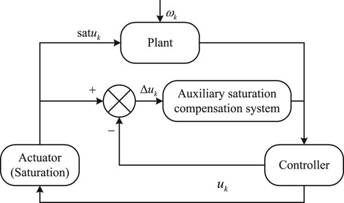
To sum up, for the nonlinear networked Markov jump systems with time delay, there are few reports to handle the resource constraints by considering the communication protocols and the dynamic quantization. In the Markov jump systems with unknown bounded nonlinearity, cumulative bounded disturbance and actuator saturation, the problems should be further discussed: the boundedness analysis of the sliding mode in finite-time and the design of an adaptive sliding mode control strategy based on auxiliary saturation compensation, etc. Therefore, the main purpose of this paper is to construct an adaptive asynchronous sliding mode controller for a class of networked discrete Markov jump systems with time-varying delay, cumulative bounded disturbance and unknown bounded nonlinear as well as actuator saturation. Firstly, the asynchronous sliding surface is designed by the hidden Markov model, which describes the asynchronous phenomenon. Secondly, under the weaker assumption for saturation function, an adaptive output feedback sliding mode control strategy with auxiliary saturation compensation systems is designed to mitigate the negative effects of saturation and chattering on the control performance of the actuator. The structure of the studied control systems is shown in Figure 1.

Figure 1. Structure diagram of networked control system based on actuator saturation.

2. Problem formulation and sliding surface design

2.1. Model description

Consider the discrete nonlinear time delay Markov jump systems with actuator saturation (1) $\{\begin{array}{rl}{x}_{k+1}& =A(r_k)x_k+A_d(r_k)x_{k-d_k}\\ & +B(r_k)(\mathrm{sat}(u_k)+f(y_k,k))\\ & +D(r_k){\omega }_k\\ y_k=& C(r_k)x_k\\ x_k=& {\varphi }_k,\mathrm{\forall }k\in [-d_M,0]\end{array}$(1) where $x_k\in {\mathbb{R}}^n$, $u_k\in {\mathbb{R}}^m$ and $y_k\in {\mathbb{R}}^p$ are the state vectors, the control input and the measurement output of the systems, respectively. $f(y_k,k)$ is an unknown nonlinear function. $d_k$ represents the varying time delay satisfying $0\le d_m\le d_k\le d_M$, here $d_M$ and $d_m$ are known upper and lower bounds of time delay. ${\varphi }_k$ denotes the initial state vector. ${\omega }_k\in {\mathbb{R}}^q$ describes the cumulative bounded disturbance input, i.e. (2) $\sum _{k=1}^N{\omega }_k^T{\omega }_k\le \delta$(2) here δ is a given positive scalar, $N\in {\mathbb{N}}^{+}$ is a known positive integer.

$\mathrm{sat}(u_k):{\mathbb{R}}^m\to {\mathbb{R}}^m$ represents the actuator saturation function, it is defined as: $\mathrm{sat}(u_k)={[\mathrm{sat}(u_{1,k}),\mathrm{sat}(u_{2,k}),\dots ,\mathrm{sat}(u_{m,k})]}^T$where $\mathrm{sat}(u_{j,k})=\mathrm{sign}(u_{j,k})\min \{u_{j,max},|u_{j,k}|\}$, $j=1,2,\dots ,m$. The constant $u_{j,max}$ denotes the saturation level of the jth input.

The stochastic processes $\{r_k=i,k\ge 0\}$ are homogeneous Markov chains taking values in the finite set ${\mathcal{N}}_1=\{1,2,\dots ,N_1\}$. The transition probability matrix is $\mathrm{\Pi }=({\pi }_{ij})$ ($\mathrm{\forall }i,j\in {\mathcal{N}}_1$), ${\pi }_{ij}\in [0,1]$, and $\sum _{j=1}^{N_1}{\pi }_{ij}=1$. For convenience, for any $r_k=i\in {\mathcal{N}}_1$, the system matrix $A(r_k)$ is denoted as $A_i$, other system matrices are similarly denoted as $A_{di}$, $B_i$, $C_i$ and $D_i$, where all of them are known matrices with appropriate dimensions. Suppose that $(A_i,B_i)$ is controllable. The input matrix $B_i$ and the output matrix $C_i$ are column full rank and row full rank, respectively. It is assumed that $\mathrm{\forall }i\in {\mathcal{N}}_1$, $\mathrm{rank}(C_i{B}_i)=m$,.

The system (1(1) $\{\begin{array}{rl}{x}_{k+1}& =A(r_k)x_k+A_d(r_k)x_{k-d_k}\\ & +B(r_k)(\mathrm{sat}(u_k)+f(y_k,k))\\ & +D(r_k){\omega }_k\\ y_k=& C(r_k)x_k\\ x_k=& {\varphi }_k,\mathrm{\forall }k\in [-d_M,0]\end{array}$(1) ) can be simplified as (3) $\{\begin{array}{rl}& x_{k+1}=A_i{x}_k+A_{di}{x}_{k-d_k}\\ & +B_i(\mathrm{sat}(u_k)+f(y_k,k))\\ & +D_i{\omega }_k\\ & y_k=C_i{x}_k\\ & x_k={\varphi }_k,\mathrm{\forall }k\in [-d_M,0]\end{array}$(3)

Assumption 2.1

The bounded matching nonlinearity $f(y_k,k)$ satisfies $\Vert f(y_k,k)\Vert \le a+b\Vert y_k\Vert$where a and b are unknown scalars.

Since $\mathrm{rank}(C_i{B}_i)=m$, it is obvious that there is a nonsingular matrix ${\mathcal{T}}_i\in {\mathbb{R}}^{n\times n}$, the system (3(3) $\{\begin{array}{rl}& x_{k+1}=A_i{x}_k+A_{di}{x}_{k-d_k}\\ & +B_i(\mathrm{sat}(u_k)+f(y_k,k))\\ & +D_i{\omega }_k\\ & y_k=C_i{x}_k\\ & x_k={\varphi }_k,\mathrm{\forall }k\in [-d_M,0]\end{array}$(3) ) can be transformed into the following form under the state transition $z_k={\mathcal{T}}_i{x}_k$, (4) $\begin{array}{rl}{z}_{k+1}& ={\overline{A}}_i{z}_k+{\overline{A}}_{di}{z}_{k-d_k}\\ & +\left[\begin{array}{c}{0}_{(n-m)\times m}\\ B_{2i}\end{array}\right](\mathrm{sat}(u_k)+f(y_k,k))\\ & +{\overline{D}}_i{\omega }_k,\end{array}$(4) (5) $\begin{array}{rl}{y}_k& =\left[\begin{array}{cc}{0}_{p\times (n-p)}& C_{2i}\end{array}\right]z_k\end{array}$(5) where $B_{2i}\in {\mathbb{R}}^{m\times m}$ and $C_{2i}\in {\mathbb{R}}^{p\times p}$ are nonsingular matrices, ${\overline{A}}_i=\left[\begin{array}{cc}{\overline{A}}_{11i}& {\overline{A}}_{12i}\\ {\overline{A}}_{21i}& {\overline{A}}_{22i}\end{array}\right]$, ${\overline{A}}_{di}=\left[\begin{array}{cc}{\overline{A}}_{d11i}& {\overline{A}}_{d12i}\\ {\overline{A}}_{d21i}& {\overline{A}}_{d22i}\end{array}\right]$, ${\overline{A}}_{11i},{\overline{A}}_{d11i}\in {\mathbb{R}}^{(n-m)\times (n-m)}$, ${\overline{A}}_{12i},{\overline{A}}_{d12i}\in {\mathbb{R}}^{(n-m)\times m}$, ${\overline{A}}_{21i},{\overline{A}}_{d21i}\in {\mathbb{R}}^{m\times (n-m)}$, ${\overline{A}}_{22i},{\overline{A}}_{d22i}\in {\mathbb{R}}^{m\times m}$, and ${\overline{D}}_i=\left[\begin{array}{c}{\overline{D}}_{1i}\\ {\overline{D}}_{2i}\end{array}\right]$, ${\overline{D}}_{1i}\in {\mathbb{R}}^{(n-m)\times q}$, ${\overline{D}}_{2i}\in {\mathbb{R}}^{m\times q}$.

With loss of generality assume $C=[0I_p]$. Since the matrix $B_i$ is column full rank in system (1), so the matrix $B_i$ can be written as $B_i=\left[\begin{array}{c}{B}_{i1}\\ B_{i2}\end{array}\right]$, where $B_{i2}$ is an invertible matrix. Let ${\mathcal{T}}_i=\left[\begin{array}{cc}I& -B_{i1}{B}_{i2}^{-1}\\ 0& I\end{array}\right]$, then ${\mathcal{T}}_i{B}_i=\left[\begin{array}{c}0\\ B_{i2}\end{array}\right]$, ${C_i\mathcal{T}}_i^{-1}=[0I_p]\left[\begin{array}{cc}I& B_{i1}{B}_{i2}^{-1}\\ 0& I\end{array}\right]=[0I_p]$.

Next, (4(4) $\begin{array}{rl}{z}_{k+1}& ={\overline{A}}_i{z}_k+{\overline{A}}_{di}{z}_{k-d_k}\\ & +\left[\begin{array}{c}{0}_{(n-m)\times m}\\ B_{2i}\end{array}\right](\mathrm{sat}(u_k)+f(y_k,k))\\ & +{\overline{D}}_i{\omega }_k,\end{array}$(4) ) can be further decomposed into the sliding mode motion (6(6) $\begin{array}{rl}{z}_{1,k+1}& ={\overline{A}}_{11i}{z}_{1,k}+{\overline{A}}_{d11i}{z}_{1,k-d_k}+{\overline{A}}_{12i}{z}_{2,k}\\ & +{\overline{A}}_{d12i}{z}_{2,k-d_k}+{\overline{D}}_{1i}{\omega }_k,\end{array}$(6) ) and the approaching motion (7(7) $\begin{array}{rl}{z}_{2,k+1}& ={\overline{A}}_{21i}{z}_{1,k}+{\overline{A}}_{d21i}{z}_{1,k-d_k}+{\overline{A}}_{22i}{z}_{2,k}\\ & +{\overline{A}}_{d22i}{z}_{2,k-d_k}+B_{2i}(\mathrm{sat}(u_k)+f(y_k,k))\\ & +{\overline{D}}_{2i}{\omega }_k\end{array}$(7) ) as follows: (6) $\begin{array}{rl}{z}_{1,k+1}& ={\overline{A}}_{11i}{z}_{1,k}+{\overline{A}}_{d11i}{z}_{1,k-d_k}+{\overline{A}}_{12i}{z}_{2,k}\\ & +{\overline{A}}_{d12i}{z}_{2,k-d_k}+{\overline{D}}_{1i}{\omega }_k,\end{array}$(6) (7) $\begin{array}{rl}{z}_{2,k+1}& ={\overline{A}}_{21i}{z}_{1,k}+{\overline{A}}_{d21i}{z}_{1,k-d_k}+{\overline{A}}_{22i}{z}_{2,k}\\ & +{\overline{A}}_{d22i}{z}_{2,k-d_k}+B_{2i}(\mathrm{sat}(u_k)+f(y_k,k))\\ & +{\overline{D}}_{2i}{\omega }_k\end{array}$(7) where $z_{1,k+1}\in {\mathbb{R}}^{n-m}$, $z_{2,k+1}\in {\mathbb{R}}^m$.

2.2. Asynchronous sliding surface synthesis

It is difficult to measure the system mode $r_k$. Therefore, the detector can be used to obtain the estimated value of $r_k$ with a certain probability (Costa et al., 2015). This leads to the fact that the system modal information of real observation from the controller is often inaccurate, i.e. the signal $l_k$ from the detector to the controller may not be synchronized with the system modal $r_k$, but they are not completely independent, and the phenomenon can be characterized by the given conditional probability. Consequently, the hidden Markov model $(r_k,l_k,{\mathcal{N}}_1,{\mathcal{N}}_2)$ is constructed to describe this asynchronous phenomenon. The random variables $l_k$ take values in ${\mathcal{N}}_2=\{1,2,\dots ,N_2\}$. The description is as follows: (8) $\mathrm{Pr}\{l_k=\mu \mid r_k=i\}={\chi }_{i\mu },\mathrm{\forall }i\in {\mathcal{N}}_1,\mu \in {\mathcal{N}}_2$(8) where, the conditional probability of modal detection ${\chi }_{i\mu }\in [0,1]$ satisfies $\sum _{\mu =1}^{N_2}{\chi }_{i\mu }=1$. The conditional probability matrix of modal detection is defined as $\mathrm{\Omega }=[{\chi }_{i\mu }]$.

Remark 2.1

Note that ${\chi }_{i\mu }$ is the probability of the systems running in the ith mode but the controller in the jth mode. Therefore, our problems are more general. The above hidden Markov model (8(8) $\mathrm{Pr}\{l_k=\mu \mid r_k=i\}={\chi }_{i\mu },\mathrm{\forall }i\in {\mathcal{N}}_1,\mu \in {\mathcal{N}}_2$(8) ) includes two cases. 1) For ${\mathcal{N}}_1={\mathcal{N}}_2$ and ${\chi }_{i\mu }=1$ when $\mu =i$, it is called modal dependence. Meanwhile, the designed controller is synchronous controller. 2) For ${\mathcal{N}}_2=1$, it is called modal independence. The controller is changed into a single-mode controller. Thus, asynchronous controller includes synchronous controller and single-mode controller.

Based on the measurement output, the following asynchronous sliding surface function is constructed (9) $s_k=[-K_{\mu }{I}_m]C_{2i}^{-1}{y}_k$(9) where $\mu \in {\mathcal{N}}_2$, $K_{\mu }$ is the parameter matrix to be designed.

Substituting (5(5) $\begin{array}{rl}{y}_k& =\left[\begin{array}{cc}{0}_{p\times (n-p)}& C_{2i}\end{array}\right]z_k\end{array}$(5) ) into (9(9) $s_k=[-K_{\mu }{I}_m]C_{2i}^{-1}{y}_k$(9) ), we can get $\begin{array}{rl}{s}_k& =\left[\begin{array}{cc}-K_{\mu }& I_m\end{array}\right]C_{2i}^{-1}\left[\begin{array}{cc}0& C_{2i}\end{array}\right]z_k\\ & =\left[\begin{array}{cc}-K_{\mu }& I_m\end{array}\right]\left[\begin{array}{ccc}{0}_{(l-m)\times (l-m)}& I_{l-m}& 0\\ 0_{m\times (n-l)}& 0& I_m\end{array}\right]z_k\\ & =\left[\begin{array}{cc}-K_{\mu }{C}_{1i}& I_m\end{array}\right]z_k\\ & =-K_{\mu }{C}_{1i}{z}_{1,k}+z_{2,k}=0\end{array}$where $C_{1i}=\left[\begin{array}{cc}{0}_{(p-m)\times (p-m)}& I_{p-m}\end{array}\right]$.

It can be seen from $s_k=0$ that $z_{2,k}=K_{\mu }{C}_{1i}{z}_{1,k}$. The sliding mode equation is obtained by substituting $z_{2,k}$ into the sliding mode motion Equation (6(6) $\begin{array}{rl}{z}_{1,k+1}& ={\overline{A}}_{11i}{z}_{1,k}+{\overline{A}}_{d11i}{z}_{1,k-d_k}+{\overline{A}}_{12i}{z}_{2,k}\\ & +{\overline{A}}_{d12i}{z}_{2,k-d_k}+{\overline{D}}_{1i}{\omega }_k,\end{array}$(6) ) (10) $z_{1,k+1}={\tilde{A}}_{1i}{z}_{1,k}+{\tilde{A}}_{d1i}{z}_{1,k-d_k}+{\overline{D}}_{1i}{\omega }_k$(10) where ${\tilde{A}}_{1i}\triangleq {\overline{A}}_{11i}+{\overline{A}}_{12i}{K}_{\mu }{C}_{1i}$, ${\tilde{A}}_{d1i}\triangleq {\overline{A}}_{d11i}+{\overline{A}}_{d12i}{K}_{\mu }{C}_{1i}$.

We definite ${\eta }_k=z_{1,k+1}-z_{1,k}$, and assume that for any $k\in \{-d_M,\dots ,0\}$, there is a positive number $b_1$ such that (11) ${\eta }_k^T{\eta }_k\le b_1.$(11)

Definition 2.1

Niu et al., 2015

Consider $N>0(N\in {\mathbb{N}}^{+})$ and non-zero disturbance ${\omega }_k$ satisfying (2(2) $\sum _{k=1}^N{\omega }_k^T{\omega }_k\le \delta$(2) ). Let scalars $c_2>c_1>0$, weighted matrix $R_i>0$. If $\mathbf{E}\{z_{1,k^{\ast }}^T{R}_i{z}_{1,k^{\ast }}\}\le c_1(\mathrm{\forall }{k}^{\ast }\in [-d_M,0])$, there are $\mathbf{E}\{z_{1,k}^T{R}_i{z}_{1,k}\}\le c_2(\mathrm{\forall }k\in [1,N])$. Then, the system (10(10) $z_{1,k+1}={\tilde{A}}_{1i}{z}_{1,k}+{\tilde{A}}_{d1i}{z}_{1,k-d_k}+{\overline{D}}_{1i}{\omega }_k$(10) ) is called stochastic finite-time bounded with respect to $(c_1,c_2,N,R_i,\delta )$.

Remark 2.2

The finite-time boundedness is different from the finite-time stability in Zuo et al. (2013). When the disturbance input is 0 (${\omega }_k=0$), the finite-time boundedness degenerates into finite-time stability. In addition, the delay systems considered in this paper are quite diverse from the systems without delay. Specifically, due to the existence of systems delays, the initial states ${\overline{\varphi }}_{1,k}$ (${\overline{\varphi }}_k={\mathcal{T}}_i{\varphi }_k$, $\mathrm{\forall }k\in [-d_M,0]$) satisfy $\mathbf{E}\{z_{1,k}^T{R}_i{z}_{1,k}\}\le c_1$. On the other hand, in order to improve the performance of Markov jump systems, it is meaningful to minimize the trajectory boundary $c_2$ and maximize the finite-time interval N.

Definition 2.2

Park et al., 2011

Let $f_1,f_2,\dots ,f_N:{\mathbb{R}}^m\mapsto {\mathbb{R}}^n$ be positive definite functions on the open subset D of ${\mathbb{R}}^m$. The interactive convex combination of the defined function on D can be expressed as $\frac{1}{{\alpha }_1}{f}_1+\frac{1}{{\alpha }_2}{f}_2+\cdots +\frac{1}{{\alpha }_N}{f}_N:D\mapsto {\mathbb{R}}^n$where ${\alpha }_i>0$ and $\sum _{i=1}^N{\alpha }_i=1$.

Lemma 2.1

Park et al., 2011

If $f_1,f_2,\dots ,f_N:{\mathbb{R}}^m\mapsto {\mathbb{R}}^n$ is a set of positive definite functions on the open subset D of ${\mathbb{R}}^m$, then the interactive convex combination of $f_i$ over D has the following properties: $\underset{{\alpha }_i}{min}\sum _{i=1}^N\frac{1}{{\alpha }_i}{f}_i(t)=\sum _{i=1}^N{f}_i(t)+\underset{g_{i,j}(t)}{max}\sum _{i\ne j}{g}_{i,j}(t)$where $g_{i,j}(t):{\mathbb{R}}^m\mapsto {\mathbb{R}}^n$, $g_{i,j}(t)=g_{j,i}(t)$, $\left[\begin{array}{cc}{f}_i(t)& g_{i,j}(t)\\ g_{j,i}(t)& f_i(t)\end{array}\right]\ge 0$, ${\alpha }_i>0$ and $\sum _{i=1}^N{\alpha }_i=1$.

Lemma 2.2

Mathiyalagan et al., 2012

For any symmetric positive definite matrix $E\in {\mathbb{R}}^{n\times n}$, the scalars ${\tau }_m$ and ${\tau }_M$ satisfy ${\tau }_m<{\tau }_M$, and the vector ${\eta }_k=x_{k+1}-x_k(k\in {\mathbb{Z}}^{+})$ as well as the following inequalities hold $\begin{array}{rl}& -\sum _{i=k-{\tau }_M}^{k-{\tau }_m-1}{\eta }_i^{T}E{\eta }_i\\ & \le -\frac{1}{{\tau }_M-{\tau }_m}\sum _{i=k-{\tau }_M}^{k-{\tau }_m-1}{\eta }_i^{T}E\sum _{i=k-{\tau }_M}^{k-{\tau }_m-1}{\eta }_i,\\ & \sum _{j=-{\tau }_M}^{-{\tau }_M-1}\sum _{i=k+j}^{k-1}{\eta }_i^{T}E{\eta }_i\\ & \le -\kappa \sum _{j=-{\tau }_M}^{-{\tau }_M-1}\sum _{i=k+j}^{k-1}{\eta }_i^{T}E\sum _{j=-{\tau }_M}^{-{\tau }_M-1}\sum _{i=k+j}^{k-1}{\eta }_i\end{array}$where $\kappa =\frac{2}{({\tau }_M-2)({\tau }_M+{\tau }_m+1)}$.

3. Stochastic finite-time boundedness analysis of sliding modes

The objectives of this section are to construct the Lyapunov–Krasovskii functional and give the sufficient condition for the stochastic finite-time boundedness of the sliding mode (10(10) $z_{1,k+1}={\tilde{A}}_{1i}{z}_{1,k}+{\tilde{A}}_{d1i}{z}_{1,k-d_k}+{\overline{D}}_{1i}{\omega }_k$(10) ) with respect to ($c_1,c_2,N,R_i,\delta$).

Theorem 3.1

For each mode $i\in {\mathcal{N}}_1$ and $\mu \in {\mathcal{N}}_2$, the scalars $\beta >1$ and $b_1>0$ are given. Suppose that the state of the system can reach the sliding surface in finite time. If there exist positive definite matrices $P_i$, $Q_{1i}$, $Q_{2i}$, $S_{1i}$, $S_{2i}$, and $W_i$, real matrix $G_i$ and positive scalars ${\lambda }_{0i}$, ${\lambda }_{1i}$, ${\lambda }_{2i}$, ${\lambda }_{3i}$, ${\lambda }_{4i}$, ${\lambda }_{5i}$ and ${\lambda }_{6i}$, such that the following inequalities (12) $\begin{array}{rl}& \left[\begin{array}{cc}{S}_{2i}& \ast \\ G& S_{2i}\end{array}\right]>0\end{array}$(12) (13) $\begin{array}{rl}& {\mathrm{\Theta }}_i=\left[\begin{array}{cccc}{\tilde{\mathrm{\Theta }}}_i& \ast & \ast & \ast \\ {\theta }_{1i}& -{\overline{P}}_i^{-1}& \ast & \ast \\ {\theta }_{2i}& 0& -S_1^{-1}& \ast \\ {\theta }_{3i}& 0& 0& -S_2^{-1}\end{array}\right]<0\end{array}$(13) (14) $\begin{array}{rl}& {\lambda }_{0i}I\le {\tilde{P}}_i\le {\lambda }_{1i}I,0<{\tilde{Q}}_{1i}\le {\lambda }_{2i}I\end{array}$(14) (15) $\begin{array}{rl}& 0<{\tilde{Q}}_{2i}\le {\lambda }_{3i}I,0<{\tilde{S}}_{1i}\le {\lambda }_{4i}I\end{array}$(15) (16) $\begin{array}{rl}& 0<{\tilde{S}}_{2i}\le {\lambda }_{5i}I,W_i\le {\lambda }_{6i}I\end{array}$(16) (17) $\begin{array}{rl}& v_1{c}_1+v_2{b}_1+{\lambda }_{6i}\delta <{\beta }^{-N}{c}_2{\lambda }_{0i}\end{array}$(17) (18) $\begin{array}{rl}& {\overline{Q}}_{1i}\triangleq \sum _{\mu =1}^{N_2}{\chi }_{i\mu }\sum _{j=1}^{N_1}{\pi }_{ij}{Q}_{1j}\end{array}$(18) (19) $\begin{array}{rl}& {\overline{Q}}_{2i}\triangleq \sum _{\mu =1}^{N_2}{\chi }_{i\mu }\sum _{j=1}^{N_1}{\pi }_{ij}{Q}_{2j}\end{array}$(19) hold, then the sliding mode (10(10) $z_{1,k+1}={\tilde{A}}_{1i}{z}_{1,k}+{\tilde{A}}_{d1i}{z}_{1,k-d_k}+{\overline{D}}_{1i}{\omega }_k$(10) ) on the sliding mode surface (9(9) $s_k=[-K_{\mu }{I}_m]C_{2i}^{-1}{y}_k$(9) ) is stochastic finite-time bounded with respect to ($c_1,c_2,N,R_i,\delta$), where $\begin{array}{rl}{\overline{P}}_i& \triangleq \sum _{\mu =1}^{N_2}{\chi }_{i\mu }\sum _{j=1}^{N_1}{\pi }_{ij}{P}_j\\ {\tilde{\mathrm{\Theta }}}_i& =\left[\begin{array}{ccccc}{\mathrm{\Theta }}_{11i}& \ast & \ast & \ast & \ast \\ \beta S_{1i}& {\mathrm{\Theta }}_{22i}& \ast & \ast & \ast \\ 0& {\mathrm{\Theta }}_{32i}& {\mathrm{\Theta }}_{33i}& \ast & \ast \\ 0& {\mathrm{\Theta }}_{42i}& {\mathrm{\Theta }}_{43i}& {\mathrm{\Theta }}_{44i}& \ast \\ 0& 0& 0& 0& -W_i\end{array}\right]<0\\ {\mathrm{\Theta }}_{11i}& =-\beta P_i+Q_{1i}+Q_{2i}-\beta S_{1i}\\ {\mathrm{\Theta }}_{22i}& =-{\beta }^{d_m}{Q}_{1i}-\beta S_{1i}-{\beta }^{d_m+1}{S}_{2i}\\ {\mathrm{\Theta }}_{32i}& ={\beta }^{d_m+1}(S_{2i}-G_i^T)\\ {\mathrm{\Theta }}_{33i}& =-{\beta }^{d_M}{Q}_{2i}-{\beta }^{d_m+1}(2S_{2i}-G_i-G_i^T)\\ {\mathrm{\Theta }}_{42i}& ={\beta }^{d_m+1}{G}_i^T\\ {\mathrm{\Theta }}_{43i}& ={\beta }^{d_m+1}(S_{2i}-G_i^T)\\ {\mathrm{\Theta }}_{44i}& =-{\beta }^{d_m+1}{S}_{2i}\\ {\theta }_{1i}& =[{\tilde{A}}_{1i}0{\tilde{A}}_{d1i}0{\overline{D}}_{1i}]\\ {\theta }_{2i}& =d_m[({\tilde{A}}_{1i}-I)0{\tilde{A}}_{d1i}0{\overline{D}}_{1i}]\\ {\theta }_{3i}& =(d_M-d_m)[({\tilde{A}}_{1i}-I)0{\tilde{A}}_{d1i}0{\overline{D}}_{1i}]\\ {\tilde{P}}_i& =R_i^{-\frac{1}{2}}{P}_i{R}_i^{-\frac{1}{2}},{\tilde{Q}}_{1i}=R_i^{-\frac{1}{2}}{Q}_{1i}{R}_i^{-\frac{1}{2}}\\ {\tilde{Q}}_{2i}& =R_i^{-\frac{1}{2}}{Q}_{2i}{R}_i^{-\frac{1}{2}},{\tilde{S}}_1=R_i^{-\frac{1}{2}}{S}_1{R}_i^{-\frac{1}{2}}\\ {\tilde{S}}_2& =R_i^{-\frac{1}{2}}{S}_2{R}_i^{-\frac{1}{2}}\\ v_1& ={\lambda }_{1i}+d_m{\beta }^{d_m-1}{\lambda }_{2i}+d_2{\beta }^{d_M-1}{\lambda }_{3i}\\ v_2& ={\beta }^{d_m-1}\frac{d_m^2(d_m-1)}{2}{\lambda }_4\\ & +{\beta }^{d_M-1}\frac{(d_M-d_m{)}^2(d_M+d_m+1)}{2}{\lambda }_5.\end{array}$

Proof.

Construct the Lyapunov–Krasovskii functional for the sliding mode (10(10) $z_{1,k+1}={\tilde{A}}_{1i}{z}_{1,k}+{\tilde{A}}_{d1i}{z}_{1,k-d_k}+{\overline{D}}_{1i}{\omega }_k$(10) ) $V(z_{1,k},i)=\sum _{h=1}^4{V}_h(z_{1,k},i)$where $\begin{array}{rl}{V}_1(z_{1,k},i)& =z_{1,k}^T{P}_i{z}_{1,k}\\ V_2(z_{1,k},i)& =\sum _{s=k-d_m}^{k-1}{\beta }^{k-1-s}{z}_{1,s}^T{Q}_{1i}{z}_{1,s}\\ & +\sum _{s=k-d_M}^{k-1}{\beta }^{k-1-s}{z}_{1,s}^T{Q}_{2i}{z}_{1,s}\\ V_3(z_{1,k},i)& =d_m\sum _{t=-d_m}^{-1}\sum _{s=k+t}^{k-1}{\beta }^{k-1-s}{\eta }_s^T{S}_{1i}{\eta }_s\\ V_4(z_{1,k},i)& =(d_M-d_m)\sum _{t=-d_M}^{-d_m-1}\sum _{s=k+t}^{k-1}{\beta }^{k-1-s}{\eta }_s^T{S}_{2i}{\eta }_s.\end{array}$Define $\mathbf{E}\{\mathrm{\Delta }{V}_h\}\triangleq \mathbf{E}\{V(z_{1,k+1},r_{k+1})|z_{1,k},r_k=i\}-V(z_k,r_k=i)$. And calculate the $\mathrm{\Delta }{V}_1$, $\mathrm{\Delta }{V}_2$, $\mathrm{\Delta }{V}_3$ and $\mathrm{\Delta }{V}_4$, respectively. We have (20) $\begin{array}{rl}\mathbf{E}\{\mathrm{\Delta }{V}_1\}& =\mathbf{E}\{V_1(k+1,z_{1,k+1},r_{k+1})\mid k,z_{1,k},r_k=i\}\\ & -V_1(k,z_{1,k},i)\\ & =\mathbf{E}\left\{z_{1,k+1}^T\left(\sum _{j=1}^{N_1}{\pi }_{ij}{P}_j\right)z_{1,k+1}\right\}\\ & -V_1(k,z_{1,k},i)\\ & =\sum _{j=1}^{N_1}{\pi }_{ij}\sum _{\mu =1}^{N_2}{\chi }_{i\mu }\{({\tilde{A}}_{1i}{z}_{1,k}+{\tilde{A}}_{d1i}{z}_{1,k-d_k}\\ & +{\overline{D}}_{1i}{\omega }_k{)}^T{P}_j({\tilde{A}}_{1i}{z}_{1,k}+{\tilde{A}}_{d1i}{z}_{1,k-d_k}\\ & +{\overline{D}}_{1i}{\omega }_k)\}-\beta V_1(k,z_{1,k},i)\\ & +(\beta -1)V_1(k,z_{1,k},i)\\ & ={\zeta }_k^T{\theta }_{1i}^T{\overline{P}}_i{\theta }_{1i}{\zeta }_k-\beta z_{1,k}^T{P}_i{z}_{1,k}\\ & +(\beta -1)V_1(k,z_{1,k},i).\end{array}$(20) where ${\zeta }_k=[z_{1,k}^T{z}_{1,k-d_m}^T{z}_{1,k-d_k}^T{z}_{1,k-d_M}^T{\omega }_k^T{]}^T$. (21) $\begin{array}{rl}\mathbf{E}\{\mathrm{\Delta }{V}_2\}& =\mathbf{E}\left\{\sum _{s=k+1-d_m}^k{\beta }^{k-s}{z}_{1,s}^T\left(\sum _{j=1}^{N_1}{\pi }_{ij}{Q}_{1j}\right)z_{1,s}\right\}\\ & -\sum _{s=k-d_m}^{k-1}{\beta }^{k-s}{z}_{1,s}^T{Q}_{1i}{z}_{1,s}\\ & +\mathbf{E}\left\{\sum _{s=k+1-d_M}^k{\beta }^{k-s}{z}_{1,s}^T\left(\sum _{j=1}^{N_1}{\pi }_{ij}{Q}_{2j}\right)z_{1,s}\right\}\\ & -\sum _{s=k-d_M}^{k-1}{\beta }^{k-s}{z}_{1,s}^T{Q}_{2i}{z}_{1,s}\\ & +(\beta -1)V_2(k,z_{1,k},i)\\ & =z_{1,k}^T\sum _{j=1}^{N_1}{\pi }_{ij}\sum _{\mu =1}^{N_2}{\chi }_{i\mu }{Q}_{1j}{z}_{1,k}\\ & +\sum _{s=k+1-d_m}^{k-1}{z}_{1,s}^T(\sum _{j=1}^{N_1}{\pi }_{ij}\sum _{\mu =1}^{N_2}{\chi }_{i\mu }{Q}_{1j}-Q_{1i})z_{1,s}\\ & -{\beta }^{d_1}{z}_{1,k-d_m}^T{Q}_{1i}{z}_{1,k-d_m}\\ & +z_{1,k}^T\sum _{j=1}^{N_1}{\pi }_{ij}\sum _{\mu =1}^{N_2}{\chi }_{i\mu }{Q}_{2j}{z}_{1,k}\\ & -{\beta }^{d_2}{z}_{1,k-d_M}^T{Q}_{2i}{z}_{1,k-d_M}\\ & +\sum _{s=k+1-d_M}^{k-1}{z}_{1,s}^T(\sum _{j=1}^{N_1}{\pi }_{ij}\sum _{\mu =1}^{N_2}{\chi }_{i\mu }{Q}_{2j}-Q_{2i})z_{1,s}\\ & +(\beta -1)V_2(k,z_{1,k},i).\end{array}$(21) When the condition (19(19) $\begin{array}{rl}& {\overline{Q}}_{2i}\triangleq \sum _{\mu =1}^{N_2}{\chi }_{i\mu }\sum _{j=1}^{N_1}{\pi }_{ij}{Q}_{2j}\end{array}$(19) ) is satisfied, according to (21(21) $\begin{array}{rl}\mathbf{E}\{\mathrm{\Delta }{V}_2\}& =\mathbf{E}\left\{\sum _{s=k+1-d_m}^k{\beta }^{k-s}{z}_{1,s}^T\left(\sum _{j=1}^{N_1}{\pi }_{ij}{Q}_{1j}\right)z_{1,s}\right\}\\ & -\sum _{s=k-d_m}^{k-1}{\beta }^{k-s}{z}_{1,s}^T{Q}_{1i}{z}_{1,s}\\ & +\mathbf{E}\left\{\sum _{s=k+1-d_M}^k{\beta }^{k-s}{z}_{1,s}^T\left(\sum _{j=1}^{N_1}{\pi }_{ij}{Q}_{2j}\right)z_{1,s}\right\}\\ & -\sum _{s=k-d_M}^{k-1}{\beta }^{k-s}{z}_{1,s}^T{Q}_{2i}{z}_{1,s}\\ & +(\beta -1)V_2(k,z_{1,k},i)\\ & =z_{1,k}^T\sum _{j=1}^{N_1}{\pi }_{ij}\sum _{\mu =1}^{N_2}{\chi }_{i\mu }{Q}_{1j}{z}_{1,k}\\ & +\sum _{s=k+1-d_m}^{k-1}{z}_{1,s}^T(\sum _{j=1}^{N_1}{\pi }_{ij}\sum _{\mu =1}^{N_2}{\chi }_{i\mu }{Q}_{1j}-Q_{1i})z_{1,s}\\ & -{\beta }^{d_1}{z}_{1,k-d_m}^T{Q}_{1i}{z}_{1,k-d_m}\\ & +z_{1,k}^T\sum _{j=1}^{N_1}{\pi }_{ij}\sum _{\mu =1}^{N_2}{\chi }_{i\mu }{Q}_{2j}{z}_{1,k}\\ & -{\beta }^{d_2}{z}_{1,k-d_M}^T{Q}_{2i}{z}_{1,k-d_M}\\ & +\sum _{s=k+1-d_M}^{k-1}{z}_{1,s}^T(\sum _{j=1}^{N_1}{\pi }_{ij}\sum _{\mu =1}^{N_2}{\chi }_{i\mu }{Q}_{2j}-Q_{2i})z_{1,s}\\ & +(\beta -1)V_2(k,z_{1,k},i).\end{array}$(21) ), we have (22) $\begin{array}{rl}\mathbf{E}\{\mathrm{\Delta }{V}_2\}& =z_{1,k}^T{Q}_{1i}{z}_{1,k}-{\beta }^{d_1}{z}_{1,k-d_m}^T{Q}_{1i}{z}_{1,k-d_m}\\ & +z_{1,k}^T{Q}_{2i}{z}_{1,k}-{\beta }^{d_M}{z}_{1,k-d_M}^T{Q}_{2i}{z}_{1,k-d_M}\\ & +(\beta -1)V_2(k,z_{1,k},i).\end{array}$(22) Similarly, it is not hard to get (23) $\begin{array}{rl}\mathbf{E}\{\mathrm{\Delta }{V}_3\}& =d_m\sum _{t=-d_m}^{-1}\sum _{s=k+1+t}^k{\beta }^{k-s}{\eta }_s^T{S}_{1i}{\eta }_s\\ & -d_m\sum _{t=-d_m}^{-1}\sum _{s=k+t}^{k-1}{\beta }^{k-s}{\eta }_s^T{S}_{1i}{\eta }_s\\ & +(\beta -1)V_3(k,z_{1,k})\\ & =d_m^2{\eta }_k^T{S}_{1i}{\eta }_k-d_m\sum _{s=k-d_m}^{k-1}{\beta }^{k-t}{\eta }_s^T{S}_{1i}{\eta }_s\\ & +(\beta -1)V_3(k,z_{1,k}).\end{array}$(23) According to Lemma 2.2, one has (24) $\begin{array}{rl}& -d_m\sum _{s=k-d_m}^{k-1}{\beta }^{k-t}{\eta }_s^T{S}_{1i}{\eta }_s\\ & \le -d_m\frac{\beta }{d_m}\left(\sum _{s=k-d_m}^{k-1}{\eta }_s^T\right)S_{1i}\left(\sum _{s=k-d_m}^{k-1}{\eta }_s\right)\\ & \le -\beta (z_{1,k}-z_{1,k-d_m}{)}^T{S}_{1i}(z_{1,k}-z_{1,k-d_m}).\end{array}$(24) Substituting (24(24) $\begin{array}{rl}& -d_m\sum _{s=k-d_m}^{k-1}{\beta }^{k-t}{\eta }_s^T{S}_{1i}{\eta }_s\\ & \le -d_m\frac{\beta }{d_m}\left(\sum _{s=k-d_m}^{k-1}{\eta }_s^T\right)S_{1i}\left(\sum _{s=k-d_m}^{k-1}{\eta }_s\right)\\ & \le -\beta (z_{1,k}-z_{1,k-d_m}{)}^T{S}_{1i}(z_{1,k}-z_{1,k-d_m}).\end{array}$(24) ) into (23(23) $\begin{array}{rl}\mathbf{E}\{\mathrm{\Delta }{V}_3\}& =d_m\sum _{t=-d_m}^{-1}\sum _{s=k+1+t}^k{\beta }^{k-s}{\eta }_s^T{S}_{1i}{\eta }_s\\ & -d_m\sum _{t=-d_m}^{-1}\sum _{s=k+t}^{k-1}{\beta }^{k-s}{\eta }_s^T{S}_{1i}{\eta }_s\\ & +(\beta -1)V_3(k,z_{1,k})\\ & =d_m^2{\eta }_k^T{S}_{1i}{\eta }_k-d_m\sum _{s=k-d_m}^{k-1}{\beta }^{k-t}{\eta }_s^T{S}_{1i}{\eta }_s\\ & +(\beta -1)V_3(k,z_{1,k}).\end{array}$(23) ) yields (25) $\begin{array}{rl}\mathbf{E}\{\mathrm{\Delta }{V}_3\}& \le -\beta (z_{1,k}-z_{1,k-{\tau }_m}{)}^T{S}_{1i}(z_{1,k}-z_{1,k-{\tau }_m})\\ & +{\zeta }_k^T{\theta }_{2i}^T{S}_{1i}{\theta }_{2i}{\zeta }_k+(\beta -1)V_3(k,z_{1,k}),\end{array}$(25) (26) $\begin{array}{rl}\mathbf{E}\{\mathrm{\Delta }{V}_4\}& =(d_M-d_m)\sum _{t=-d_M}^{-d_m-1}\sum _{s=k+t+1}^k{\beta }^{k-s}{\eta }_s^T{S}_{2i}{\eta }_s\\ & +(\beta -1)V_4(k,z_{1,k})\\ & -(d_M-d_m)\sum _{t=-d_M}^{-d_m-1}\sum _{s=k+t}^{k-1}{\beta }^{k-s}{\eta }_s^T{S}_{2i}{\eta }_s\\ & =(d_M-d_m{)}^2{\eta }_k^T{S}_{2i}{\eta }_k\\ & -(d_M-d_m)\sum _{t=k-d_M}^{k-d_m-1}{\beta }^{k-t}{\eta }_t^T{S}_{2i}{\eta }_t\\ & +(\beta -1)V_4(k,z_{1,k}).\end{array}$(26) According to Lemmas 2.1 and 2.2, the interactive convex combination method is used to deal with the second item of (26(26) $\begin{array}{rl}\mathbf{E}\{\mathrm{\Delta }{V}_4\}& =(d_M-d_m)\sum _{t=-d_M}^{-d_m-1}\sum _{s=k+t+1}^k{\beta }^{k-s}{\eta }_s^T{S}_{2i}{\eta }_s\\ & +(\beta -1)V_4(k,z_{1,k})\\ & -(d_M-d_m)\sum _{t=-d_M}^{-d_m-1}\sum _{s=k+t}^{k-1}{\beta }^{k-s}{\eta }_s^T{S}_{2i}{\eta }_s\\ & =(d_M-d_m{)}^2{\eta }_k^T{S}_{2i}{\eta }_k\\ & -(d_M-d_m)\sum _{t=k-d_M}^{k-d_m-1}{\beta }^{k-t}{\eta }_t^T{S}_{2i}{\eta }_t\\ & +(\beta -1)V_4(k,z_{1,k}).\end{array}$(26) ), one has $\begin{array}{rl}& -(d_M-d_m)\sum _{t=k-d_M}^{k-d_m-1}{\beta }^{k-t}{\eta }_t^T{S}_{2i}{\eta }_t\\ & \le -(d_M-d_m)\sum _{t=k-d_M}^{k-d_k-1}{\beta }^{d_m+1}{\eta }_t^T{S}_{2i}{\eta }_t\\ & -(d_M-d_m)\sum _{t=k-d_k}^{k-d_m-1}{\beta }^{d_m+1}{\eta }_t^T{S}_{2i}{\eta }_t\\ & \le -{\beta }^{d_1+1}\frac{d_M-d_m}{d_M-d_k}\sum _{t=k-d_M}^{k-d_k-1}{\eta }_t^T{S}_{2i}\sum _{t=k-d_M}^{k-d_k-1}{\eta }_t\\ & -{\beta }^{d_1+1}\frac{d_M-d_m}{d_k-d_m}\sum _{t=k-d_k}^{k-d_m-1}{\eta }_t^T{S}_{2i}\sum _{t=k-d_k}^{k-d_m-1}{\eta }_t.\end{array}$Further, the above formula is represented as (27) $\begin{array}{rl}& -(d_M-d_m)\sum _{t=k-d_M}^{k-d_m-1}{\beta }^{k-t}{\eta }_t^T{S}_{2i}{\eta }_t\\ & \le -{\beta }^{d_m+1}\left\{{\tilde{W}}_k^T\left[\begin{array}{cc}{S}_{2i}& \ast \\ G_i& S_{2i}\end{array}\right]{\tilde{W}}_k\right\}.\end{array}$(27) where ${\tilde{W}}_k=\left[\begin{array}{c}{z}_{1,k-d_k}-z_{1,k-d_M}\\ z_{1,k-d_m}-z_{1,k-d_k}\end{array}\right]$.

Substituting (27(27) $\begin{array}{rl}& -(d_M-d_m)\sum _{t=k-d_M}^{k-d_m-1}{\beta }^{k-t}{\eta }_t^T{S}_{2i}{\eta }_t\\ & \le -{\beta }^{d_m+1}\left\{{\tilde{W}}_k^T\left[\begin{array}{cc}{S}_{2i}& \ast \\ G_i& S_{2i}\end{array}\right]{\tilde{W}}_k\right\}.\end{array}$(27) ) into (26(26) $\begin{array}{rl}\mathbf{E}\{\mathrm{\Delta }{V}_4\}& =(d_M-d_m)\sum _{t=-d_M}^{-d_m-1}\sum _{s=k+t+1}^k{\beta }^{k-s}{\eta }_s^T{S}_{2i}{\eta }_s\\ & +(\beta -1)V_4(k,z_{1,k})\\ & -(d_M-d_m)\sum _{t=-d_M}^{-d_m-1}\sum _{s=k+t}^{k-1}{\beta }^{k-s}{\eta }_s^T{S}_{2i}{\eta }_s\\ & =(d_M-d_m{)}^2{\eta }_k^T{S}_{2i}{\eta }_k\\ & -(d_M-d_m)\sum _{t=k-d_M}^{k-d_m-1}{\beta }^{k-t}{\eta }_t^T{S}_{2i}{\eta }_t\\ & +(\beta -1)V_4(k,z_{1,k}).\end{array}$(26) ), we get (28) $\begin{array}{rl}\mathbf{E}\{\mathrm{\Delta }{V}_4\}& \le -{\beta }^{d_m+1}\left\{{\tilde{z}}_{1,k}^T{\mathcal{H}}_i{\tilde{z}}_{1,k}^T\right\}+{\zeta }_k^T{\theta }_{3i}^T{S}_{2i}{\theta }_{3i}{\zeta }_k\\ & +(\beta -1)V_4(k,z_{1,k}).\end{array}$(28) where $\begin{array}{rl}{\tilde{z}}_{1,k}& =[z_{1,k-d_m}^T{z}_{1,k-d_k}^T{z}_{1,k-d_M}^T{]}^T\\ {\mathcal{H}}_i& =\left[\begin{array}{ccc}{S}_{2i}& \ast & \ast \\ G_i^T-S_{2i}& 2S_{2i}-G_i-G_i^T& \ast \\ -G_i^T& -S_{2i}+G_i^T& S_{2i}\end{array}\right]\end{array}$Next, construct an auxiliary function $J_k=\mathbf{E}\{\mathrm{\Delta }{V}_k-(\beta -1)V_k-{\omega }_k^T{W}_i{\omega }_k\}.$Combining with (20(20) $\begin{array}{rl}\mathbf{E}\{\mathrm{\Delta }{V}_1\}& =\mathbf{E}\{V_1(k+1,z_{1,k+1},r_{k+1})\mid k,z_{1,k},r_k=i\}\\ & -V_1(k,z_{1,k},i)\\ & =\mathbf{E}\left\{z_{1,k+1}^T\left(\sum _{j=1}^{N_1}{\pi }_{ij}{P}_j\right)z_{1,k+1}\right\}\\ & -V_1(k,z_{1,k},i)\\ & =\sum _{j=1}^{N_1}{\pi }_{ij}\sum _{\mu =1}^{N_2}{\chi }_{i\mu }\{({\tilde{A}}_{1i}{z}_{1,k}+{\tilde{A}}_{d1i}{z}_{1,k-d_k}\\ & +{\overline{D}}_{1i}{\omega }_k{)}^T{P}_j({\tilde{A}}_{1i}{z}_{1,k}+{\tilde{A}}_{d1i}{z}_{1,k-d_k}\\ & +{\overline{D}}_{1i}{\omega }_k)\}-\beta V_1(k,z_{1,k},i)\\ & +(\beta -1)V_1(k,z_{1,k},i)\\ & ={\zeta }_k^T{\theta }_{1i}^T{\overline{P}}_i{\theta }_{1i}{\zeta }_k-\beta z_{1,k}^T{P}_i{z}_{1,k}\\ & +(\beta -1)V_1(k,z_{1,k},i).\end{array}$(20) )–(28(28) $\begin{array}{rl}\mathbf{E}\{\mathrm{\Delta }{V}_4\}& \le -{\beta }^{d_m+1}\left\{{\tilde{z}}_{1,k}^T{\mathcal{H}}_i{\tilde{z}}_{1,k}^T\right\}+{\zeta }_k^T{\theta }_{3i}^T{S}_{2i}{\theta }_{3i}{\zeta }_k\\ & +(\beta -1)V_4(k,z_{1,k}).\end{array}$(28) ), ${\mathrm{\Omega }}_i={\tilde{\mathrm{\Theta }}}_i+{\theta }_{1i}^T{\overline{P}}_i{\theta }_{1i}+{\theta }_{2i}^T{S}_{1i}{\theta }_{2i}+{\theta }_{3i}^T{S}_{2i}{\theta }_{3i}<0$ can ensure $J_k<0$. Further, we are not hard to get $\mathbf{E}\{V_{k+1}\}-V_k\le (\beta -1)V_k+{\omega }_k^T{W}_i{\omega }_k$, that is, (29) $\mathbf{E}\{V_{k+1}\}\le \beta V_k+{\lambda }_{max}(W_i)\mathbf{E}\{{\omega }_k^T{\omega }_k\}.$(29) Summing $\mathbf{E}\{V_{k+1}\}$ from 0 to k−1 yields (30) $\begin{array}{rl}\mathbf{E}\{V_k\}& \le {\beta }^k\mathbf{E}\{V_0\}\\ & +{\lambda }_{max}(W_i)\mathbf{E}\left\{\sum _{j=0}^{k-1}{\beta }^{k-1-j}{\omega }_k^T{\omega }_k\right\}\\ & \le {\beta }^k\mathbf{E}\{V_0\}+{\lambda }_{max}(W_i){\beta }^k\delta .\end{array}$(30) On the other hand, for $x_k={\varphi }_k$ ($k\in [-d_M,0]$), we have (31) $\begin{array}{rl}\mathbf{E}\{V_0\}& =z_{1,0}^T{P}_i{z}_{1,0}+\sum _{s=-d_m}^{-1}{\beta }^{-1-s}{z}_{1,s}^T{Q}_{1i}{z}_{1,s}\\ & +\sum _{s=-d_M}^{-1}{\beta }^{-1-s}{z}_{1,s}^T{Q}_{2i}{z}_{1,s}\\ & +d_m\sum _{t=-d_m}^{-1}\sum _{s=t}^{-1}{\beta }^{-1-s}{\eta }_s^T{S}_{1i}{\eta }_s\\ & +(d_M-d_m)\sum _{t=-d_M}^{-d_m-1}\sum _{s=t}^{-1}{\beta }^{-1-s}{\eta }_s^T{S}_{2i}{\eta }_s\\ & \le {\lambda }_{max}({\tilde{P}}_i)z_{1,0}^T{R}_i{z}_{1,0}\\ & +{\beta }^{d_m-1}{\lambda }_{max}({\tilde{Q}}_{1i})\sum _{s=-d_m}^{-1}{z}_{1,s}^T{R}_i{z}_{1,s}\\ & +{\beta }^{d_M-1}{\lambda }_{max}({\tilde{Q}}_{2i})\sum _{s=-d_M}^{-1}{z}_{1,s}^T{R}_i{z}_{1,s}\\ & +(d_M-d_m){\beta }^{d_M-1}{\lambda }_{max}({\tilde{S}}_{2i})\sum _{t=-d_M}^{-d_m-1}\sum _{s=t}^{-1}{\eta }_s^T{\eta }_s\\ & +d_m{\beta }^{d_m-1}{\lambda }_{max}({\tilde{S}}_{1i})\sum _{t=-d_m}^{-1}\sum _{s=t}^{-1}{\eta }_s^T{\eta }_s.\end{array}$(31) According to (11(11) ${\eta }_k^T{\eta }_k\le b_1.$(11) ) and Definition 2.1, it is easy to obtain (32) $\mathbf{E}\{V_0\}\le v_1{c}_1+v_2{b}_1.$(32) In addition, (33) $\begin{array}{rl}\mathbf{E}\{V_k\}& \ge \mathbf{E}\{z_{1,k}^T{P}_i{z}_{1,k}\}\\ & =\mathbf{E}\left\{z_{1,k}^T{R}_i^{\frac{1}{2}}{\tilde{P}}_i{R}_i^{\frac{1}{2}}{z}_{1,k}\right\}\\ & \ge {\lambda }_{max}({\tilde{P}}_i)\mathbf{E}\{z_{1,k}^T{R}_i{z}_{1,k}\}.\end{array}$(33) Therefore (34) $\begin{array}{rl}\mathbf{E}\{z_{1,k}^T{R}_i{z}_{1,k}\}& \le {\beta }^k\frac{v_1{c}_1+v_2{b}_1+{\lambda }_{max}(W_i)\delta }{{\lambda }_{min}({\tilde{P}}_i)}\\ & <{\beta }^k\frac{v_1{c}_1+v_2{b}_1+{\lambda }_6\delta }{{\lambda }_{0i}}<c_2.\end{array}$(34) The proof is complete.

4. Sliding mode controller design and reachability analysis

4.1. Design of adaptive sliding mode controller with saturation compensation

In this section, an adaptive sliding mode controller is constructed and an auxiliary saturation compensation system is designed to mitigate the negative effects of actuator saturation.

Similar to Yao et al. (2018) and Zhang and Xia (2010), define a small neighbourhood $\mathbb{S}$ near the sliding surface before designing the controller (35) $\mathbb{S}=\{z_k\in {\mathbb{R}}^n:\Vert z_k\Vert \le \sigma \},k\in [-d_2,N]$(35) where $\sigma >0$ is an unknown parameter.

Aiming at the nonlinear problem in the system (3(3) $\{\begin{array}{rl}& x_{k+1}=A_i{x}_k+A_{di}{x}_{k-d_k}\\ & +B_i(\mathrm{sat}(u_k)+f(y_k,k))\\ & +D_i{\omega }_k\\ & y_k=C_i{x}_k\\ & x_k={\varphi }_k,\mathrm{\forall }k\in [-d_M,0]\end{array}$(3) ), the following adaptive output feedback sliding mode controller with saturation compensation is designed based on the asynchronous sliding mode surface (9(9) $s_k=[-K_{\mu }{I}_m]C_{2i}^{-1}{y}_k$(9) ) (36) $u_k=u_{k1}+u_{k2}$(36) where $u_{k1}=-B_{2i}^{-1}[\gamma s_k+\Vert [-K_{\mu }{C}_{1i}{I}_m]({\overline{A}}_i+{\overline{A}}_{di})\Vert \frac{s_k}{\Vert s_k\Vert +{\vartheta }_1}{\hat{\sigma }}_k]-\frac{B_{2i}^T{s}_k}{\Vert B_{2i}^T{s}_k\Vert +{\vartheta }_2}({\hat{a}}_k+{\hat{b}}_k\Vert y_k\Vert )$, $u_{k2}=-B_{2i}^{-1}\tilde{K}{\psi }_k$.

The following adaptive laws are designed in the small neighbourhood defined by (35(35) $\mathbb{S}=\{z_k\in {\mathbb{R}}^n:\Vert z_k\Vert \le \sigma \},k\in [-d_2,N]$(35) ) (37) $\begin{array}{rl}\mathrm{\Delta }{\hat{a}}_k& =q_0(-{ϵ}_0{\hat{a}}_k+\Vert B_{2i}^T{s}_k\Vert )\\ \mathrm{\Delta }{\hat{b}}_k& =q_1(-{ϵ}_1{\hat{b}}_k+\Vert B_{2i}^T{s}_k\Vert \Vert y_k\Vert )\\ \mathrm{\Delta }{\hat{\sigma }}_k& =q_2[-{ϵ}_2{\hat{\sigma }}_k+\Vert [-K_{\mu }{C}_{1i}{I}_m]({\overline{A}}_i\\ & +{\overline{A}}_{di})\Vert \Vert s_k\Vert ]\end{array}$(37) where $K_{\mu }$ and $\tilde{K}$ are symmetric positive definite matrices, ${\vartheta }_1$, ${\vartheta }_2$ are smaller positive scalars, γ, ${ϵ}_0$, ${ϵ}_1$, ${ϵ}_2$, $q_0$, $q_1$ and $q_2$ are positive scalars, ${\hat{a}}_k$, ${\hat{b}}_k$ and ${\hat{\sigma }}_k$ are the estimate values for unknown parameters a, b and σ, respectively. Besides, $\mathrm{\Delta }{\hat{a}}_k={\hat{a}}_{k+1}-{\hat{a}}_k$, $\mathrm{\Delta }{\hat{b}}_k={\hat{b}}_{k+1}-{\hat{b}}_k$ and $\mathrm{\Delta }{\hat{\sigma }}_k={\hat{\sigma }}_{k+1}-{\hat{\sigma }}_k$.

To compensate the effect of the actuator saturation, the variable ${\psi }_k$ in $u_2$ is obtained from the following auxiliary system (38) $\begin{array}{rl}\mathrm{\Delta }{\psi }_k& =e_2\mathrm{\Delta }{u}_k-e_1{\psi }_k\\ & -\frac{\Vert s_k^T{B}_{2i}\mathrm{\Delta }{u}_k{\Vert }_1+0.5e_2\mathrm{\Delta }{u}_k^T\mathrm{\Delta }{u}_k}{\Vert {\psi }_k{\Vert }^2}{\psi }_k\end{array}$(38) where $e_1$ and $e_2$ are positive constants.

Remark 4.1

In general, the symbolic function is used to design sliding mode controller when analysing the reachability of sliding surface. It usually exists in the form of $s_{k}sign(s_k)=\frac{s_k^T{s}_k}{\Vert s_k\Vert }$, where $\frac{s_k^T{s}_k}{\Vert s_k\Vert }$ is a discontinuous term. To reduce the chattering caused by the discontinuous term, the $\frac{s_k^T{s}_k}{\Vert s_k\Vert +\theta }$ is use to replace the $\frac{s_k^T{s}_k}{\Vert s_k\Vert }$. Therefore, there is no symbolic function in the design of the controller. Specifically, the controller without symbolic function is designed by replacing discontinuous functions $\frac{s_k}{\Vert s_k\Vert }$ and $\frac{B_{2i}^T{s}_k}{\Vert B_{2i}^T{s}_k\Vert }$ with $\frac{s_k}{\Vert s_k\Vert +{\vartheta }_1}$ and $\frac{B_{2i}^T{s}_k}{\Vert B_{2i}^T{s}_k\Vert +{\vartheta }_2}$ in this paper, respectively. Design $u_2$ can compensate the negative effects of actuator saturation. By adjusting the parameter $e_2$ in the auxiliary system (38(38) $\begin{array}{rl}\mathrm{\Delta }{\psi }_k& =e_2\mathrm{\Delta }{u}_k-e_1{\psi }_k\\ & -\frac{\Vert s_k^T{B}_{2i}\mathrm{\Delta }{u}_k{\Vert }_1+0.5e_2\mathrm{\Delta }{u}_k^T\mathrm{\Delta }{u}_k}{\Vert {\psi }_k{\Vert }^2}{\psi }_k\end{array}$(38) ), the overcompensation can be avoided for the actuator saturation phenomenon.

4.2. Reachability analysis of the sliding mode motion

Suppose that the parameter σ is unknown, the reachability of sliding mode surface is discussed under the adaptive sliding mode controller (36(36) $u_k=u_{k1}+u_{k2}$(36) ) based on the Lyapunov method.

According to (4(4) $\begin{array}{rl}{z}_{k+1}& ={\overline{A}}_i{z}_k+{\overline{A}}_{di}{z}_{k-d_k}\\ & +\left[\begin{array}{c}{0}_{(n-m)\times m}\\ B_{2i}\end{array}\right](\mathrm{sat}(u_k)+f(y_k,k))\\ & +{\overline{D}}_i{\omega }_k,\end{array}$(4) ) and (9(9) $s_k=[-K_{\mu }{I}_m]C_{2i}^{-1}{y}_k$(9) ), $s_k=[-K_{\mu }{C}_{1i}{I}_m]z_k$, it is not difficult to get (39) $\begin{array}{rl}{s}_{k+1}& =[-K_{\mu }{C}_{1i}{I}_m]\{{\overline{A}}_i{z}_k+{\overline{A}}_{di}{z}_{k-d_k}\\ & +\left[\begin{array}{c}0\\ B_{2i}\end{array}\right](\mathrm{sat}(u_k)+f(y_k,k))\\ & +{\overline{D}}_i{\omega }_k\}.\end{array}$(39)

Theorem 4.1

Consider the discrete nonlinear Markov jump systems (4(4) $\begin{array}{rl}{z}_{k+1}& ={\overline{A}}_i{z}_k+{\overline{A}}_{di}{z}_{k-d_k}\\ & +\left[\begin{array}{c}{0}_{(n-m)\times m}\\ B_{2i}\end{array}\right](\mathrm{sat}(u_k)+f(y_k,k))\\ & +{\overline{D}}_i{\omega }_k,\end{array}$(4) ) with saturation and time-varying delay, suppose that the gain matrix $K_{\mu }$ has a feasible solution in the asynchronous sliding mode surface (9(9) $s_k=[-K_{\mu }{I}_m]C_{2i}^{-1}{y}_k$(9) ). For $\mathrm{\forall }i\in {\mathcal{N}}_1$ and $\mu \in {\mathcal{N}}_2$, scalars γ, $e_1$ and $e_2$, design the sliding mode controller (36(36) $u_k=u_{k1}+u_{k2}$(36) ) based on the adaptive law (37(37) $\begin{array}{rl}\mathrm{\Delta }{\hat{a}}_k& =q_0(-{ϵ}_0{\hat{a}}_k+\Vert B_{2i}^T{s}_k\Vert )\\ \mathrm{\Delta }{\hat{b}}_k& =q_1(-{ϵ}_1{\hat{b}}_k+\Vert B_{2i}^T{s}_k\Vert \Vert y_k\Vert )\\ \mathrm{\Delta }{\hat{\sigma }}_k& =q_2[-{ϵ}_2{\hat{\sigma }}_k+\Vert [-K_{\mu }{C}_{1i}{I}_m]({\overline{A}}_i\\ & +{\overline{A}}_{di})\Vert \Vert s_k\Vert ]\end{array}$(37) ) and the auxiliary system (38(38) $\begin{array}{rl}\mathrm{\Delta }{\psi }_k& =e_2\mathrm{\Delta }{u}_k-e_1{\psi }_k\\ & -\frac{\Vert s_k^T{B}_{2i}\mathrm{\Delta }{u}_k{\Vert }_1+0.5e_2\mathrm{\Delta }{u}_k^T\mathrm{\Delta }{u}_k}{\Vert {\psi }_k{\Vert }^2}{\psi }_k\end{array}$(38) ), if there exist positive definite matrix $\tilde{K}$ satisfying $-\frac{1}{2}\tilde{K}+e_1{I}_m-\frac{1}{2}{e}_2{I}_m>0$, then the states of the system (4(4) $\begin{array}{rl}{z}_{k+1}& ={\overline{A}}_i{z}_k+{\overline{A}}_{di}{z}_{k-d_k}\\ & +\left[\begin{array}{c}{0}_{(n-m)\times m}\\ B_{2i}\end{array}\right](\mathrm{sat}(u_k)+f(y_k,k))\\ & +{\overline{D}}_i{\omega }_k,\end{array}$(4) ) would be driven onto near $z_k\in \mathbb{S}$.

Proof.

Consider the Lyapunov function ${\tilde{V}}_k=\frac{1}{2}\{s_k^T{s}_k+\frac{1}{q_0}{\tilde{a}}_k^2+\frac{1}{q_1}{\tilde{b}}_k^2+\frac{1}{q_2}{\tilde{\sigma }}_k^2+{\psi }_k^T{\psi }_k\}$where ${\tilde{a}}_k=a-{\hat{a}}_k$, ${\tilde{b}}_k=b-{\hat{b}}_k$ and ${\tilde{\sigma }}_k=\sigma -{\hat{\sigma }}_k$ represent the estimation errors of a, b and σ, respectively.

The increment $\mathrm{\Delta }{\tilde{V}}_k$ can be obtained by a simple calculation (40) $\begin{array}{rl}\mathbf{E}\{\mathrm{\Delta }{\tilde{V}}_k\}& =\mathbf{E}\{s_k^T\mathrm{\Delta }{s}_k+\frac{1}{q_0}{\tilde{a}}_k\mathrm{\Delta }{\hat{a}}_k+\frac{1}{q_1}{\tilde{b}}_k\mathrm{\Delta }{\hat{b}}_k\\ & +\frac{1}{q_2}{\tilde{\sigma }}_k\mathrm{\Delta }{\hat{\sigma }}_k+{\psi }_k^T\mathrm{\Delta }{\psi }_k\}+\mathrm{{\rm Y}}.\end{array}$(40) where $\begin{array}{rl}\mathrm{\Delta }{s}_k& =s_{k+1}-s_k,\mathrm{\Delta }{\tilde{a}}_k={\tilde{a}}_{k+1}-{\tilde{a}}_k\\ \mathrm{\Delta }{\tilde{b}}_k& ={\tilde{b}}_{k+1}-{\tilde{b}}_k,\mathrm{\Delta }{\tilde{\sigma }}_k={\tilde{\sigma }}_{k+1}-{\tilde{\sigma }}_k\\ \mathrm{\Delta }{\psi }_k& ={\psi }_{k+1}-{\psi }_k\\ \mathrm{{\rm Y}}& =\frac{1}{2}(\mathrm{\Delta }{s}_k^T\mathrm{\Delta }{s}_k+\frac{1}{q_0}\mathrm{\Delta }{\tilde{a}}_k^2+\frac{1}{q_1}\mathrm{\Delta }{\tilde{b}}_k^2\\ & +\frac{1}{q_2}\mathrm{\Delta }{\tilde{\sigma }}_k^2+\mathrm{\Delta }{\psi }_k^T\mathrm{\Delta }{\psi }_k).\end{array}$It is worth noting that $\mathrm{\Delta }{\tilde{a}}_k=-\mathrm{\Delta }{\hat{a}}_k$, $\mathrm{\Delta }{\tilde{b}}_k=-\mathrm{\Delta }{\hat{b}}_k$ and $\mathrm{\Delta }{\tilde{\sigma }}_k=-\mathrm{\Delta }{\hat{\sigma }}_k$, then (41) $\begin{array}{rl}\mathbf{E}\{\mathrm{\Delta }{\tilde{V}}_k\}& =\mathbf{E}\{s_k^T\mathrm{\Delta }{s}_k-\frac{1}{q_0}{\tilde{a}}_k\mathrm{\Delta }{\hat{a}}_k-\frac{1}{q_1}{\tilde{b}}_k\mathrm{\Delta }{\hat{b}}_k\\ & -\frac{1}{q_2}{\tilde{\sigma }}_k\mathrm{\Delta }{\hat{\sigma }}_k+{\psi }_k^T\mathrm{\Delta }{\psi }_k\}+\mathrm{{\rm Y}}.\end{array}$(41) Letting $\mathrm{\Delta }{u}_k=\mathrm{sat}(u_k)-u_k$, by substituting the adaptive laws (37(37) $\begin{array}{rl}\mathrm{\Delta }{\hat{a}}_k& =q_0(-{ϵ}_0{\hat{a}}_k+\Vert B_{2i}^T{s}_k\Vert )\\ \mathrm{\Delta }{\hat{b}}_k& =q_1(-{ϵ}_1{\hat{b}}_k+\Vert B_{2i}^T{s}_k\Vert \Vert y_k\Vert )\\ \mathrm{\Delta }{\hat{\sigma }}_k& =q_2[-{ϵ}_2{\hat{\sigma }}_k+\Vert [-K_{\mu }{C}_{1i}{I}_m]({\overline{A}}_i\\ & +{\overline{A}}_{di})\Vert \Vert s_k\Vert ]\end{array}$(37) ) and (39(39) $\begin{array}{rl}{s}_{k+1}& =[-K_{\mu }{C}_{1i}{I}_m]\{{\overline{A}}_i{z}_k+{\overline{A}}_{di}{z}_{k-d_k}\\ & +\left[\begin{array}{c}0\\ B_{2i}\end{array}\right](\mathrm{sat}(u_k)+f(y_k,k))\\ & +{\overline{D}}_i{\omega }_k\}.\end{array}$(39) ) into (41(41) $\begin{array}{rl}\mathbf{E}\{\mathrm{\Delta }{\tilde{V}}_k\}& =\mathbf{E}\{s_k^T\mathrm{\Delta }{s}_k-\frac{1}{q_0}{\tilde{a}}_k\mathrm{\Delta }{\hat{a}}_k-\frac{1}{q_1}{\tilde{b}}_k\mathrm{\Delta }{\hat{b}}_k\\ & -\frac{1}{q_2}{\tilde{\sigma }}_k\mathrm{\Delta }{\hat{\sigma }}_k+{\psi }_k^T\mathrm{\Delta }{\psi }_k\}+\mathrm{{\rm Y}}.\end{array}$(41) ), we have $\begin{array}{rl}\mathbf{E}\{\mathrm{\Delta }{\tilde{V}}_k\}& =s_k^T[-K_{\mu }{C}_{1i}{I}_m]({\overline{A}}_i{z}_k+{\overline{A}}_{di}{z}_{k-d_k})\\ & +s_k^T{B}_{2i}{u}_k+s_k^T{B}_{2i}\mathrm{\Delta }{u}_k+s_k^T{B}_{2i}f(y_k,k)\\ & +s_k^T[-K_{\mu }{C}_{1i}{I}_m]{\overline{D}}_i{\omega }_k-s_k^T{s}_k\\ & -\frac{1}{q_0}{\tilde{a}}_k{q}_0(-{ϵ}_0{\hat{a}}_k+\Vert B_{2i}^T{s}_k\Vert )\\ & -\frac{1}{q_1}{\tilde{b}}_k{q}_1(-{ϵ}_1{\hat{b}}_k+\Vert B_{2i}^T{s}_k\Vert \Vert y_k\Vert )\\ & -\frac{1}{q_2}{\tilde{\sigma }}_k{q}_2(-{ϵ}_2{\hat{\sigma }}_k\\ & +\Vert [-K_{\mu }{C}_{1i}{I}_m]({\overline{A}}_i+{\overline{A}}_{di})\Vert \Vert s_k\Vert \\ & +{\psi }_k^T\mathrm{\Delta }{\psi }_k)+\mathrm{{\rm Y}}.\end{array}$Combine Assumption 2.1, the controller (36(36) $u_k=u_{k1}+u_{k2}$(36) ) with the auxiliary system (38(38) $\begin{array}{rl}\mathrm{\Delta }{\psi }_k& =e_2\mathrm{\Delta }{u}_k-e_1{\psi }_k\\ & -\frac{\Vert s_k^T{B}_{2i}\mathrm{\Delta }{u}_k{\Vert }_1+0.5e_2\mathrm{\Delta }{u}_k^T\mathrm{\Delta }{u}_k}{\Vert {\psi }_k{\Vert }^2}{\psi }_k\end{array}$(38) ), we can obtain (42) $\begin{array}{rl}\mathbf{E}\{\mathrm{\Delta }{\tilde{V}}_k\}& \le s_k^T(\gamma I+I)s_k-s_k^T\tilde{K}{\psi }_k+s_k^T{B}_{2i}\mathrm{\Delta }{u}_k\\ & -\Vert [-K_{\mu }{C}_{1i}{I}_m]{\overline{D}}_i\Vert \Vert {\omega }_k\Vert \Vert s_k\Vert \\ & -\Vert [-K_{\mu }{C}_{1i}{I}_m]({\overline{A}}_i+{\overline{A}}_{di})\Vert \Vert s_k\Vert {\hat{\sigma }}_k\\ & +s_k^T[-K_{\mu }{C}_{1i}{I}_m]{\overline{D}}_i{\omega }_k\\ & +\sigma \Vert [-K_{\mu }{C}_{1i}{I}_m]({\overline{A}}_i+{\overline{A}}_{di})\Vert \Vert s_k\Vert \\ & -\Vert B_{2i}^T{s}_k\Vert ({\hat{a}}_k+{\hat{b}}_k\Vert y_k\Vert )\\ & +\Vert s_k^T{B}_{2i}\Vert (a+b\Vert y_k\Vert )-{ϵ}_0{({\hat{a}}_k-\frac{a}{2})}^2\\ & +\frac{1}{4}{ϵ}_0{a}^2-(a-{\hat{a}}_k)\Vert B_{2i}^T{s}_k\Vert +\frac{1}{4}{ϵ}_1{b}^2\\ & -{ϵ}_1{({\hat{b}}_k-\frac{b}{2})}^2-(b-{\hat{b}}_k)\Vert B_{2i}^T{s}_k\Vert \Vert y_k\Vert \\ & -{ϵ}_2{({\hat{\sigma }}_k-\frac{\sigma }{2})}^2+\frac{1}{4}{ϵ}_2{\sigma }^2-\Vert s_k^T{B}_{2i}\mathrm{\Delta }{u}_k{\Vert }_1\\ & -(\sigma -{\hat{\sigma }}_k)\Vert [-K_{\mu }{C}_{1i}{I}_m]({\overline{A}}_i\\ & +{\overline{A}}_{di})\Vert \Vert s_k\Vert -e_1{\psi }_k^T{\psi }_k+e_2{\psi }_k^T\mathrm{\Delta }{u}_k\\ & -\frac{1}{2}{e}_2\mathrm{\Delta }{u}_k^T\mathrm{\Delta }{u}_k+\mathrm{{\rm Y}}.\end{array}$(42) According to the fundamental inequality and norm properties, there are (43) $\begin{array}{rl}{s}_k^T{B}_{2i}\mathrm{\Delta }{u}_k& \le \Vert s_k^T{B}_{2i}\mathrm{\Delta }{u}_k{\Vert }_1\\ s_k^T\tilde{K}{\psi }_k& \le \frac{1}{2}{s}_k^T\tilde{K}{s}_k+\frac{1}{2}{\psi }_k^T\tilde{K}{\psi }_k\\ {\psi }_k^T\mathrm{\Delta }{u}_k& \le \frac{1}{2}{\psi }_k^T{\psi }_k+\frac{1}{2}\mathrm{\Delta }{u}_k^T\mathrm{\Delta }{u}_k.\end{array}$(43) Then, (42(42) $\begin{array}{rl}\mathbf{E}\{\mathrm{\Delta }{\tilde{V}}_k\}& \le s_k^T(\gamma I+I)s_k-s_k^T\tilde{K}{\psi }_k+s_k^T{B}_{2i}\mathrm{\Delta }{u}_k\\ & -\Vert [-K_{\mu }{C}_{1i}{I}_m]{\overline{D}}_i\Vert \Vert {\omega }_k\Vert \Vert s_k\Vert \\ & -\Vert [-K_{\mu }{C}_{1i}{I}_m]({\overline{A}}_i+{\overline{A}}_{di})\Vert \Vert s_k\Vert {\hat{\sigma }}_k\\ & +s_k^T[-K_{\mu }{C}_{1i}{I}_m]{\overline{D}}_i{\omega }_k\\ & +\sigma \Vert [-K_{\mu }{C}_{1i}{I}_m]({\overline{A}}_i+{\overline{A}}_{di})\Vert \Vert s_k\Vert \\ & -\Vert B_{2i}^T{s}_k\Vert ({\hat{a}}_k+{\hat{b}}_k\Vert y_k\Vert )\\ & +\Vert s_k^T{B}_{2i}\Vert (a+b\Vert y_k\Vert )-{ϵ}_0{({\hat{a}}_k-\frac{a}{2})}^2\\ & +\frac{1}{4}{ϵ}_0{a}^2-(a-{\hat{a}}_k)\Vert B_{2i}^T{s}_k\Vert +\frac{1}{4}{ϵ}_1{b}^2\\ & -{ϵ}_1{({\hat{b}}_k-\frac{b}{2})}^2-(b-{\hat{b}}_k)\Vert B_{2i}^T{s}_k\Vert \Vert y_k\Vert \\ & -{ϵ}_2{({\hat{\sigma }}_k-\frac{\sigma }{2})}^2+\frac{1}{4}{ϵ}_2{\sigma }^2-\Vert s_k^T{B}_{2i}\mathrm{\Delta }{u}_k{\Vert }_1\\ & -(\sigma -{\hat{\sigma }}_k)\Vert [-K_{\mu }{C}_{1i}{I}_m]({\overline{A}}_i\\ & +{\overline{A}}_{di})\Vert \Vert s_k\Vert -e_1{\psi }_k^T{\psi }_k+e_2{\psi }_k^T\mathrm{\Delta }{u}_k\\ & -\frac{1}{2}{e}_2\mathrm{\Delta }{u}_k^T\mathrm{\Delta }{u}_k+\mathrm{{\rm Y}}.\end{array}$(42) ) can be simplified as $\begin{array}{rl}\mathbf{E}\{\mathrm{\Delta }{\tilde{V}}_k\}& \le -s_k^T(\gamma I_m+I_m-\frac{1}{2}\tilde{K})s_k-{ϵ}_2{({\hat{\sigma }}_k-\frac{\sigma }{2})}^2\\ & -{ϵ}_0{({\hat{a}}_k-\frac{a}{2})}^2-{ϵ}_1{({\hat{b}}_k-\frac{b}{2})}^2\\ & -{\psi }_k^T(-\frac{1}{2}\tilde{K}+e_1{I}_m-\frac{1}{2}{e}_{2}I){\psi }_k\\ & +\frac{1}{4}{ϵ}_1{b}^2+\frac{1}{4}{ϵ}_2{\sigma }^2+\frac{1}{4}{ϵ}_0{a}^2+\mathrm{{\rm Y}}.\end{array}$ Select the parameters $e_1$ and $e_2$, such that $e_1{I}_m-\frac{1}{2}\tilde{K}-\frac{1}{2}{e}_2{I}_m>0$, and then (44) $\begin{array}{rl}\mathbf{E}\{\mathrm{\Delta }{\tilde{V}}_k\}& \le -s_k^T(\gamma I_m+I_m-\frac{1}{2}\tilde{K})s_k-{ϵ}_2{({\hat{\sigma }}_k-\frac{\sigma }{2})}^2\\ & -{ϵ}_0{({\hat{a}}_k-\frac{a}{2})}^2-{ϵ}_1{({\hat{b}}_k-\frac{b}{2})}^2+\frac{1}{4}{ϵ}_1{b}^2\\ & +\frac{1}{4}{ϵ}_2{\sigma }^2+\frac{1}{4}{ϵ}_0{a}^2+\mathrm{{\rm Y}}.\end{array}$(44) The parameter γ can be selected according to the practical situation. When the sliding function $s_k$ tends to the small bounded neighbourhood near the equilibrium point, $\mathbf{E}\{\mathrm{\Delta }{\tilde{V}}_k\}<0$ can be guaranteed by adjusting γ. Therefore, according to literatures (Wang & Liu, 2018; Yao et al., 2018), under the controller (36(36) $u_k=u_{k1}+u_{k2}$(36) ), the state trajectories of the system (4(4) $\begin{array}{rl}{z}_{k+1}& ={\overline{A}}_i{z}_k+{\overline{A}}_{di}{z}_{k-d_k}\\ & +\left[\begin{array}{c}{0}_{(n-m)\times m}\\ B_{2i}\end{array}\right](\mathrm{sat}(u_k)+f(y_k,k))\\ & +{\overline{D}}_i{\omega }_k,\end{array}$(4) ) can be driven to the small neighbourhood $\mathbb{S}$ near the sliding surface and kept on it all the time.

4.3. Solve the parameters

Note that the conditions given in Theorem 3.1 are not linear matrix inequalities. Next, the nonlinear coupling terms in inequality (13(13) $\begin{array}{rl}& {\mathrm{\Theta }}_i=\left[\begin{array}{cccc}{\tilde{\mathrm{\Theta }}}_i& \ast & \ast & \ast \\ {\theta }_{1i}& -{\overline{P}}_i^{-1}& \ast & \ast \\ {\theta }_{2i}& 0& -S_1^{-1}& \ast \\ {\theta }_{3i}& 0& 0& -S_2^{-1}\end{array}\right]<0\end{array}$(13) ) are dealt with.

Theorem 4.2

For given positive scalars $c_2>c_1$, $\beta >1$ and positive definite matrix $R_i$, each mode $i\in {\mathcal{N}}_1$ and $\mu \in {\mathcal{N}}_2$, assume that there exist positive definite matrices $P_i$, $Q_{1i}$, $Q_{2i}$, $S_{1i}$, $S_{2i}$, $W_i$, real matrix $G_i$ and positive scalars ${\lambda }_{0i}$, ${\lambda }_{1i}$, ${\lambda }_{2i}$, ${\lambda }_{3i}$, ${\lambda }_{4i}$, ${\lambda }_{5i}$ and ${\lambda }_{6i}$, such that the following inequalities are solvable (45) $\begin{array}{rl}& \left[\begin{array}{cc}{S}_{2i}& \ast \\ G_i& S_{2i}\end{array}\right]>0\end{array}$(45) (46) $\begin{array}{rl}& {\mathrm{\Omega }}_i=\left[\begin{array}{cccc}{\mathrm{\Theta }}_i& \ast & \ast & \ast \\ {\theta }_{1i}& {\mathrm{\Omega }}_{22i}& \ast & \ast \\ {\theta }_{2i}& 0& {\mathrm{\Omega }}_{33i}& \ast \\ {\theta }_{3i}& 0& 0& {\mathrm{\Omega }}_{44i}\end{array}\right]<0\end{array}$(46) (47) $\begin{array}{rl}& {\lambda }_{0i}{R}_i\le P_i\le {\lambda }_{1i}{R}_i,0<Q_{1i}\le {\lambda }_{2i}{R}_i\end{array}$(47) (48) $\begin{array}{rl}& 0<Q_{2i}\le {\lambda }_{3i}{R}_i,0<S_{1i}\le {\lambda }_{4i}{R}_i\end{array}$(48) (49) $\begin{array}{rl}& 0<S_{2i}\le {\lambda }_{5i}{R}_i,W_i\le {\lambda }_{6i}{I}_n\end{array}$(49) (50) $\begin{array}{rl}& v_1{c}_1+v_2{b}_1+{\overline{\lambda }}_{2i}\delta <{\beta }^{-N}{c}_2{\lambda }_{0i}.\end{array}$(50) where $\begin{array}{rl}{\mathrm{\Omega }}_{22i}& =-2I_{n-m}+{\overline{P}}_i,{\mathrm{\Omega }}_{33i}=-2I_{n-m}+S_{1i}\\ {\mathrm{\Omega }}_{44i}& =-2I_{n-m}+S_{2i}\end{array}$Then, the sliding mode (11(11) ${\eta }_k^T{\eta }_k\le b_1.$(11) ) on the sliding surface (9(9) $s_k=[-K_{\mu }{I}_m]C_{2i}^{-1}{y}_k$(9) ) is robust stochastic finite-time bounded with respect to ($c_1,c_2,N,R_i,\delta$). Further, the output feedback gain matrix $K_{\mu }$ can be obtained by solving (45(45) $\begin{array}{rl}& \left[\begin{array}{cc}{S}_{2i}& \ast \\ G_i& S_{2i}\end{array}\right]>0\end{array}$(45) )–(50(50) $\begin{array}{rl}& v_1{c}_1+v_2{b}_1+{\overline{\lambda }}_{2i}\delta <{\beta }^{-N}{c}_2{\lambda }_{0i}.\end{array}$(50) ).

Proof.

With the help of $(I_{n-m}-{\overline{P}}_i){\overline{P}}_i^{-1}(I_{n-m}-{\overline{P}}_i)\ge 0$, we can get $-{\overline{P}}_i^{-1}\le -2I_{n-m}+{\overline{P}}_i.$Similarly, we have $-S_{1i}^{-1}\le -2I_{n-m}+S_{1i}$ and $-S_{2i}^{-1}\le -2I_{n-m}+S_{2i}$. Therefore, the matrix inequality (13(13) $\begin{array}{rl}& {\mathrm{\Theta }}_i=\left[\begin{array}{cccc}{\tilde{\mathrm{\Theta }}}_i& \ast & \ast & \ast \\ {\theta }_{1i}& -{\overline{P}}_i^{-1}& \ast & \ast \\ {\theta }_{2i}& 0& -S_1^{-1}& \ast \\ {\theta }_{3i}& 0& 0& -S_2^{-1}\end{array}\right]<0\end{array}$(13) ) can be transformed into (46(46) $\begin{array}{rl}& {\mathrm{\Omega }}_i=\left[\begin{array}{cccc}{\mathrm{\Theta }}_i& \ast & \ast & \ast \\ {\theta }_{1i}& {\mathrm{\Omega }}_{22i}& \ast & \ast \\ {\theta }_{2i}& 0& {\mathrm{\Omega }}_{33i}& \ast \\ {\theta }_{3i}& 0& 0& {\mathrm{\Omega }}_{44i}\end{array}\right]<0\end{array}$(46) ).

Remark 4.2

In Theorem 3.1, $c_2$ depends on the values of $c_1$, β, and N. For given β and N, if $c_1$ is fixed, then the minimum value of $c_2$ can be obtained by solving the following optimization problem $\begin{array}{rl}& min{c}_2\\ & \mathrm{s}.\mathrm{t}.(45)--(50).\end{array}$According to Theorem 4.2, we know that $c_2$ exist in the form of linear in the inequalities 45(45) $\begin{array}{rl}& \left[\begin{array}{cc}{S}_{2i}& \ast \\ G_i& S_{2i}\end{array}\right]>0\end{array}$(45) )–(50(50) $\begin{array}{rl}& v_1{c}_1+v_2{b}_1+{\overline{\lambda }}_{2i}\delta <{\beta }^{-N}{c}_2{\lambda }_{0i}.\end{array}$(50) ). Therefore, the optimization problem ‘$min{c}_2$, s.t. 45(45) $\begin{array}{rl}& \left[\begin{array}{cc}{S}_{2i}& \ast \\ G_i& S_{2i}\end{array}\right]>0\end{array}$(45) )–(50(50) $\begin{array}{rl}& v_1{c}_1+v_2{b}_1+{\overline{\lambda }}_{2i}\delta <{\beta }^{-N}{c}_2{\lambda }_{0i}.\end{array}$(50) )’ is a convex optimization problem, which can be solved by using the convex optimization toolbox in Matlab to obtain the minimum value of $c_2$.

5. Numerical simulation and analysis

In this section, a numerical example is given to illustrate the advantages of the designed controller based on an auxiliary saturation compensation system.

Consider the discrete Markov jump systems with two modes, and the controller also has two modes, that is ${\mathcal{N}}_1=\{1,2\}$ and ${\mathcal{N}}_2=\{1,2\}$, transition probability matrix $\mathrm{\Pi }=\left[\begin{array}{cc}0.8& 0.2\\ 0.4& 0.6\end{array}\right]$, modal detection conditional probability matrix $\mathrm{\Omega }=\left[\begin{array}{cc}0.3& 0.7\\ 0.6& 0.4\end{array}\right]$. The following system parameters in (4(4) $\begin{array}{rl}{z}_{k+1}& ={\overline{A}}_i{z}_k+{\overline{A}}_{di}{z}_{k-d_k}\\ & +\left[\begin{array}{c}{0}_{(n-m)\times m}\\ B_{2i}\end{array}\right](\mathrm{sat}(u_k)+f(y_k,k))\\ & +{\overline{D}}_i{\omega }_k,\end{array}$(4) ) are selected $\begin{array}{rl}{\overline{A}}_1& =\left[\begin{array}{ccc}0.695& -0.05& 0.0792\\ -0.205& 0.95& 0.62\\ 0.01& 0& 0.98\end{array}\right]\\ {\overline{A}}_2& =\left[\begin{array}{ccc}0.9& 0.2& 0.9\\ -0.3& 0.37& 0.2\\ 0.8& 0.1& 0.82\end{array}\right]\\ {\overline{A}}_{d1}& =\left[\begin{array}{ccc}0.1& 0.02& 0.029\\ 0.05& 0.01& 0.04\\ 0.03& 0.01& 0.01\end{array}\right]\\ {\overline{A}}_{d2}& =\left[\begin{array}{ccc}0.01& -0.02& 0.054\\ 0.034& 0.01& 0.034\\ -0.04& 0.01& 0.001\end{array}\right]\\ B_{21}& =0.1,B_{22}=0.9,C_{21}=C_{22}=I_2\\ {\overline{D}}_1& =\left[\begin{array}{c}1\\ 1\\ 1\end{array}\right],{\overline{D}}_2=\left[\begin{array}{c}0\\ 0.1\\ 0.1\end{array}\right]\end{array}$and the nonlinear function $f(y_k,k)=0.3\sin (3k)y_{1,k}$.

The time-varying delay is selected as $d_k\in [2,5]$, the initial values of the system states are $z_k=[1.93-0.9{]}^T(k\in [-5,0])$, the upper bound of the cumulative bounded disturbance is $\delta =1$, N = 50 and the saturation level is ${\mu }_{j,max}=1.3$.

Let $c_1=1$, $c_2=15$, $\gamma =1.01$, $e_1=1$,$e_2=0.1$, ${\vartheta }_1={\vartheta }_2=1$, $\beta =1.001$, $b_1=0.01$ and positive definite matrix $R_1=R_2=\mathrm{diag}\{0.1,0.07\}$. Give the initial value of the adaptive laws ${\hat{a}}_0=0.058$, ${\hat{b}}_0=0.0275$, ${\hat{\sigma }}_0=0.05$. Obviously, the initial values satisfy $z_{1,k}^T{R}_i{z}_{1,k}\le c_1$, ${\eta }_k^T{\eta }_k\le b_1(k\in [-5,0])$.

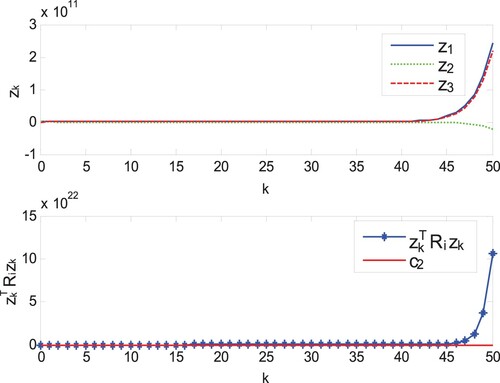
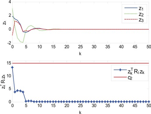
Figure 2 shows the modal evolution of the systems and the controller under asynchronous control strategy. The trajectories of $z_k$ and sliding mode $z_k^T{R}_i{z}_k$ in the open-loop system (4(4) $\begin{array}{rl}{z}_{k+1}& ={\overline{A}}_i{z}_k+{\overline{A}}_{di}{z}_{k-d_k}\\ & +\left[\begin{array}{c}{0}_{(n-m)\times m}\\ B_{2i}\end{array}\right](\mathrm{sat}(u_k)+f(y_k,k))\\ & +{\overline{D}}_i{\omega }_k,\end{array}$(4) ) are shown in Figure 3. It is obvious that the systems are unstable without sliding mode control.

Figure 2. Mode evolution of system and controller.

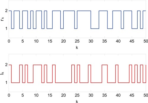
Figure 3. The trajectories $z_k$ and $z_{1,k}^T{R}_i{z}_{1,k}$ of open-loop system.

For given parameters ${ϵ}_0={ϵ}_1={ϵ}_2=1$, $q_0=q_1=q_2=1$, by solving Theorem 4.2, we obtain the controller parameters: $K_1=-0.1377$, $K_2=0.0136$ and $\tilde{K}=0.9498$. According to whether the saturation phenomenon is compensated, the control performance is discussed in two cases for the adaptive output feedback sliding mode controller system (36(36) $u_k=u_{k1}+u_{k2}$(36) ).

Case 1: There is the phenomenon of actuator saturation but not compensated saturation. Under the controller $u_k=u_{1,k}$, the simulation results are shown in Figures 4–6.

Figure 4. The trajectories $z_k$ and $z_{1,k}^T{R}_i{z}_{1,k}$ of closed-loop system in Case 1.

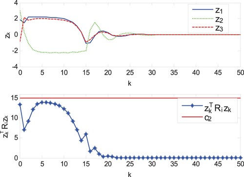
Figure 5. Control input $u_k$ and sliding variable $s_k$ in Case 1.

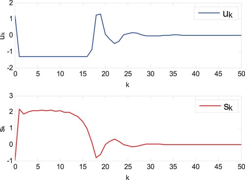
Figure 6. The trajectories of estimation parameters ${\hat{a}}_k$, ${\hat{b}}_k$ and ${\hat{\sigma }}_k$ in Case 1.

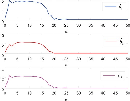
Figure 7. The trajectories $z_k$ and $z_{1,k}^T{R}_i{z}_{1,k}$ of closed-loop system in Case 2.

Case 2: The auxiliary system (38(38) $\begin{array}{rl}\mathrm{\Delta }{\psi }_k& =e_2\mathrm{\Delta }{u}_k-e_1{\psi }_k\\ & -\frac{\Vert s_k^T{B}_{2i}\mathrm{\Delta }{u}_k{\Vert }_1+0.5e_2\mathrm{\Delta }{u}_k^T\mathrm{\Delta }{u}_k}{\Vert {\psi }_k{\Vert }^2}{\psi }_k\end{array}$(38) ) is designed to compensate the actuator saturation phenomenon. Under the adaptive sliding mode controller (36(36) $u_k=u_{k1}+u_{k2}$(36) ), the simulation results are shown in Figures 7–9.

Figure 8. Control input $u_k$ and sliding variable $s_k$ in Case 2.

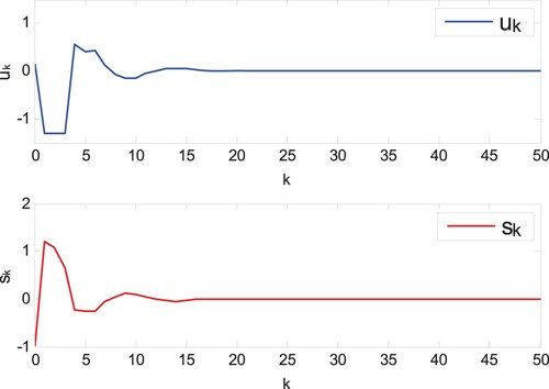
Figure 9. The trajectories of estimation parameters ${\hat{a}}_k$, ${\hat{b}}_k$ and ${\hat{\sigma }}_k$ in Case 2.

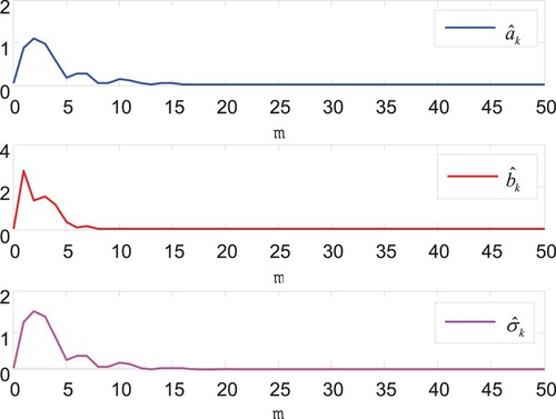
It can be clearly seen that in Case 1, although the states can be driven to the origin in Figures 4–6, the unknown parameters can be estimated effectively, but compared with Figures 7–9 in Case 2, the actuator saturation phenomenon leads to poor control performance and slower convergence speed. Therefore, the designed control strategy based on the new auxiliary saturation compensation system has the obvious control effect in this paper. The phenomenon of input saturation in Figures 4 and 7 roughly occurs in intervals $[216]$ and $[23]$, respectively. It can be seen that the design auxiliary system can reduce the impact of saturation through compensation. The simulation results verify the superiority and necessity of the design method.

6. Conclusions

For the actuator saturation phenomenon, based on the auxiliary saturation compensation system, the adaptive asynchronous sliding mode control problem has been studied for a class of networked discrete time-delay Markov jump systems with bounded noise and unknown disturbance. Firstly, since the system mode is not easy to get accurately, by using the hidden Markov model, the asynchronous sliding surface has been designed based on the measured output, and the sliding equation has been obtained. Moreover, the Lyapunov–Krasovskii functional has been constructed, and the criterion of the sliding mode stochastic finite-time boundedness has been given. Secondly, in the case that the sliding mode region is bounded but the upper bound is unknown, in order to reduce the chattering and the negative impact caused by the actuator saturation, an adaptive output feedback sliding mode controller without the sign function has been designed via the auxiliary saturation compensation, which ensures that the system state trajectories can reach the sliding region and remain in the small neighbourhood. Finally, the effectiveness of the proposed control strategy has been verified by the numerical simulations.

Disclosure statement

No potential conflict of interest was reported by the authors.

Data availability statement

All data generated or analyzed during this study are included in this published article.

Additional information

Funding

This work was supported by the National Natural Science Foundation of China [grant number 12071102].

References

- Amato, F., & Ariola, M. (2005). Finite-time control of discrete-time linear systems. IEEE Transactions on Automatic Control, 50(5), 724–729. https://doi.org/https://doi.org/10.1109/TAC.2005.847042
- Costa, O. L. D. V., Fragoso, M. D., & Todorov, M. G. (2015). A detector-based approach for the H2 control of Markov jump linear systems with partial information. IEEE Transactions on Automatic Control, 60(5), 1219–1234. https://doi.org/https://doi.org/10.1109/TAC.2014.2366253
- Ding, Z., Wei, G., & Ding, X. (2014). Speed identification and control for permanent magnet synchronous motor via sliding mode approach. Systems Science and Control Engineering, 2(1), 161–167. https://doi.org/https://doi.org/10.1080/21642583.2014.886974
- Du, C., Yang, C., Li, F., & Gui, W. (2019). A novel asynchronous control for artificial delayed Markovian jump systems via output feedback sliding mode approach. IEEE Transactions on Systems Man and Cybernetics-Systems, 49(2), 364–374. https://doi.org/https://doi.org/10.1109/TSMC.2018.2815032
- Guan, C., Fei, Z., & Yang, T. (2019). Necessary and sufficient criteria for asynchronous stabilization of Markovian jump systems. Journal of the Franklin Institute, 356(3), 1468–1483. https://doi.org/https://doi.org/10.1016/j.jfranklin.2018.11.025
- Guo, X., Zhao, J., Li, H., Wang, J., Liao, F., & Chen, Y. (2020). Novel auxiliary saturation compensation design for neuroadaptive NTSM tracking control of high speed trains with actuator saturation. Journal of the Franklin Institute, 357(3), 1582–1602. https://doi.org/https://doi.org/10.1016/j.jfranklin.2019.11.006
- Han, F., He, Q., Gao, H., Song, J., & Li, J. (2020). Decouple design of leader-following consensus control for nonlinear multi-agent systems. Systems Science and Control Engineering, 8(1), 288–296. https://doi.org/https://doi.org/10.1080/21642583.2020.1748138
- Hu, J., Wang, Z., Gao, H., & Stergioulas, L. K. (2012). Robust sliding mode control for discrete stochastic systems with mixed time delays, randomly occurring uncertainties, and randomly occurring nonlinearities. IEEE Transactions on Industrial Electronics, 59(7), 3008–3015. https://doi.org/https://doi.org/10.1109/TIE.2011.2168791
- Janardhanan, S., & Bandyopadhyay, B. (2006). Discrete sliding mode control of systems with unmatched uncertainty using multirate output feedback. IEEE Transactions on Automatic Control, 51(6), 1030–1035. https://doi.org/https://doi.org/10.1109/TAC.2006.876810
- Jenabzadeh, A., & Safarinejadian, B. (2018). Distributed tracking control problem of lipschitz multi-agent systems with external disturbances and input delay. Systems Science and Control Engineering, 6(1), 268–278. https://doi.org/https://doi.org/10.1080/21642583.2018.1485060
- Jia, S., & Shan, J. (2020). Finite-time trajectory tracking control of space manipulator under actuator saturation. IEEE Transactions on Industrial Electronics, 67(3), 2086–2096. https://doi.org/https://doi.org/10.1109/TIE.41
- Kapila, V., & Haddad, W. M. (2000). Fixed-structure controller design for systems with actuator amplitude and rate non-linearities. International Journal of Control, 73(6), 520–530. https://doi.org/https://doi.org/10.1080/002071700219524
- Liu, L., Wang, Y., Ma, L., Zhang, J., & Bo, Y. (2018). Robust finite-horizon filtering for nonlinear time-delay Markovian jump systems with weighted try-once-discard protocol. Systems Science and Control Engineering, 6(1), 180–194. https://doi.org/https://doi.org/10.1080/21642583.2018.1474396
- Liu, Q., Wang, Z., He, X., & Zhou, D. (2014). A survey of event-based strategies on control and estimation. Systems Science and Control Engineering, 2(1), 90–97. https://doi.org/https://doi.org/10.1080/21642583.2014.880387
- Ma, Y., & Liu, J. (2020). Adaptive diffusion strategies with Markov jump over networks. Systems Science and Control Engineering, 8(1), 388–404. https://doi.org/https://doi.org/10.1080/21642583.2020.1784808
- Mathiyalagan, K., Sakthivel, R., & Anthoni, S. M. (2012). New robust passivity criteria for discrete-time genetic regulatory networks with Markovian jumping parameters. Canadian Journal of Physics, 90(2), 107–118. https://doi.org/https://doi.org/10.1139/p11-147
- Niu, Y., Zou, Y., & Song, J. (2015). Robust finite-time bounded control for discrete-time stochastic systems with communication constraint. IET Control Theory and Applications, 9(13), 2015–2021. https://doi.org/https://doi.org/10.1049/cth2.v9.13
- Park, P., Ko, J. W., & Jeong, C. (2011). Reciprocally convex approach to stability of systems with time-varying delays. Automatica, 47(1), 235–238. https://doi.org/https://doi.org/10.1016/j.automatica.2010.10.014
- Shang, H., & Zong, G. (2020). Event-triggered sliding mode control under the Round-Robin protocol for networked switched systems. Nonlinear Dynamics, 100(3), 2401–2413. https://doi.org/https://doi.org/10.1007/s11071-020-05618-2
- Song, H., Chen, S., & Yam, Y. (2017). Sliding mode control for discrete-time systems with Markovian packet dropouts. IEEE Transactions on Cybernetics, 47(11), 3669–3679. https://doi.org/https://doi.org/10.1109/TCYB.2016.2577340
- Song, J., Niu, Y., & Zou, Y. (2017). Asynchronous output feedback control of time-varying Markovian jump systems within a finite-time interval. Journal of the Franklin Institute, 354 (15), 6747–6765. https://doi.org/https://doi.org/10.1016/j.jfranklin.2017.08.028
- Song, J., Niu, Y., & Zou, Y. (2018). Asynchronous sliding mode control of Markovian jump systems with time-varying delays and partly accessible mode detection probabilities. Automatica, 93(8), 33–41. https://doi.org/https://doi.org/10.1016/j.automatica.2018.03.037
- Song, J., Wang, Z., & Niu, Y. (2018). Static output-feedback sliding mode control under Round-Robin protocol. International Journal of Robust and Nonlinear Control, 28(18), 5841–5857. https://doi.org/https://doi.org/10.1002/rnc.v28.18
- Wang, J., & Liu, C. (2018). Stabilization of uncertain systems with Markovian modes of time delay and quantization density. IEEE/CAA Journal of Automatica Sinica, 5(2), 463–470. https://doi.org/https://doi.org/10.1109/JAS.2017.7510823
- Wu, X., & Mu, X. (2019). Event-triggered control for networked nonlinear semi-Markovian jump systems with randomly occurring uncertainties and transmission delay. Information Sciences, 487(4), 84–96. https://doi.org/https://doi.org/10.1016/j.ins.2019.03.014
- Xia, Y., Zhu, Z., Li, C., Yang, H., & Zhu, Q. (2010). Robust adaptive sliding mode control for uncertain discrete-time systems with time delay. Journal of the Franklin Institute, 347(1), 339–357. https://doi.org/https://doi.org/10.1016/j.jfranklin.2009.10.011
- Yang, S., & Lin, L. (2019). Dynamic output feedback finite-horizon control for Markov jump systems with actuator saturations. IEEE Access, 7, 132587–132593. https://doi.org/https://doi.org/10.1109/Access.6287639
- Yao, D., Ren, H., Li, P., & Zhou, Q. (2018). Sliding mode output-feedback control of discrete-time Markov jump systems using singular system method. Journal of the Franklin Institute, 355(13), 5576–5591. https://doi.org/https://doi.org/10.1016/j.jfranklin.2018.06.007
- Zha, L., Fang, J., Li, X., & Liu, J. (2017). Event-triggered output feedback H∞ control for networked Markovian jump systems with quantizations. Nonlinear Analysis: Hybrid Systems, 24(8), 146–158. https://doi.org/https://doi.org/10.1016/j.nahs.2016.10.002
- Zhan, S., Lam, J., & Xiong, J. (2010). Static output-feedback stabilization of discrete-time Markovian jump linear systems: A system augmentation approach. Automatica, 46(4), 687–694. https://doi.org/https://doi.org/10.1016/j.automatica.2010.02.001
- Zhang, H., & Shen, M. (2019). Sliding mode H∞ control of time-varying delay Markov jump with quantized output. Optimal Control Applications and Methods, 40(2), 226–240. https://doi.org/https://doi.org/10.1002/oca.v40.2
- Zhang, J., & Xia, Y. (2010). Design of static output feedback sliding mode control for uncertain linear systems. IEEE Transactions on Industrial Electronics, 57(6), 2161–2170. https://doi.org/https://doi.org/10.1109/TIE.2009.2033485
- Zheng, B., Yang, G., & Li, T. (2014). Quantised feedback sliding mode control of linear uncertain systems. IET Control Theory and Applications, 8(7), 479–487. https://doi.org/https://doi.org/10.1049/cth2.v8.7
- Zuo, Z., Li, H., & Wang, Y. (2013). New criterion for finite-time stability of linear discrete-time systems with time-varying delay. Journal of the Franklin Institute, 350(9), 2745–2756. https://doi.org/https://doi.org/10.1016/j.jfranklin.2013.06.017