Stability comparison of different controllers for hydraulic turbine fractional order interval parameter time-delay system

Abstract

This paper studies the stability comparison of four controllers for a hydraulic turbine fractional order interval parameter time-delay system. Considering the terms of parameter uncertainty and time-lag, the hydraulic turbine fractional order interval parameter time-delay system is established by using fractional calculus and identification technology. Through the edge theorem and D-decomposition method, the calculation process of controller parameter stability region is derived in every detail. Subsequently, the four different controllers including the PID, PID plus second order derivative (PID2D), fractional order PID (FOPID) and fractional order PID plus second order derivative (FOPID2D) controllers, are applied in the hydraulic turbine fractional order interval parameter time-delay system. According to the experimental results, the effect of the controller parameters k_d, k_d2, α and λ on the stability region of the parameters k_p and k_i is analysed and the variable law of stability regions of the hydraulic turbine governing system is presented. Finally, the stability region of these four controllers is compared and the results validate the superiority of the FOPID2D controller over the other controllers.

KEYWORDS:

• Hydraulic turbine governing system
• stability region
• fractional order
• controller parameter
• time-delay
• interval parameter

1. Introduction

The hydraulic turbine governing system (HTGS) is a complicated closed-loop system which mainly consists of the controller, actuator, hydraulic turbine-penstock and generator-load. This system is occasionally influenced by hydraulic, mechanical and electric factors (Wei, 2011). In the HTGS system, the hydroelectric generating unit (HGU) can be regarded as the controlled object of the turbine governor. Thus, the control performance of closed-loop system is essential to the strong guarantee of a stable and safe power supply (Li & Zhou, 2011). However, the controller parameters need to be changed or modified accordingly in a variety of changing operating conditions. The stability regions of closed-loop system are inseparably linked to the regulation of the hydraulic turbine governing system. Therefore, the determination of stability region intuitively and conveniently provides an effective reference for the engineers. And it is important in guiding the stable and safe operation of hydropower plants.

The HTGS system usually operates in multiple operating environments. This may cause the constructed model parameters, especially the linearized model parameters, change along with the operating-points. And the identified or measured parameter values need a complex solving process including the complicated calculation and the numeral error. The performance analysis and control of systems are difficult when the parameters perturb uncertainly (Petras et al., 2004). Therefore, it is necessary to propose a stability determination approach for the HTGS system with the interval parameters. Beyond that, the two terms of time-lag and fractional order are considered in the system modelling of HTGS. On one hand, in the hydraulic actuator, the time delay easily occurs during the process of signal transmission between the different hydraulic components. This can cause a delay in the guide vane opening to the large and frequent load disturbance (Xu et al., 2015). For this reason, the time-lag of the actuator is an important consideration in the modelling of HTGS. On the other hand, due to the unique advantages of high flexibility and long-term memory, the fractional model is getting considerable attention from scholars and experts with the development of fractional order theory (Xian et al., 2019). It has been used in the system modelling and controller design of several fields (Chen et al., 2014). Compared to the integer order models, the fractional order model has a stronger description ability and a wider range of applications. This suggests that it is necessary to establish the fractional order mathematical model to describe the dynamic characteristics of the hydraulic turbine governing system.

In recent years, it has appeared some research work on the stability of the HTGS system. Xu B et.al built a fractional order hydraulic turbine model and analysed the effect of fractional order parameters and water hammer parameters on the system’s stability (Xu et al., 2015). The dynamic characteristics of the system were studied via the bifurcation graphs and time waveforms. Using a novel Hamiltonian function, Xu B et.al presented a Hamiltonian mathematical model of HTGS considering the fractional order and time-delay (Xu et al., 2017). Then the influence of fractional order parameters and time-delay parameters on the system dynamic response was discussed by simulation experiments. Long Y et.al presented the motion laws of the bifurcation points and chaotic regions with the changing fractional order by the results of fractional bifurcation diagrams, time waveforms, and phase orbits. And the stable range of k_d was gained by the various fractional-order values (Long et al., 2018). The studies mentioned above paid attention to the impact of the typical parameters of controlled objects on the system stability. Several cut-off points between the stable region and unstable region were achieved using the bifurcation theory and Poincare map in mathematics. Unlike those studies, the research in this text uses three different controllers besides the traditional PID (proportional integral differential) controller and takes the system parameter uncertainty into consideration. It focuses on the stability region procedure of controller parameters for the hydraulic turbine fractional interval parameter time-delay system. Then the variable law of stability regions with different controller parameter values is summarized. Finally, the stability comparison of various controllers is carried out.

With the exception of the classic PID controller, several developed controllers namely the fractional order PID (FOPID) and PID plus second order derivative (PID2D) have been proposed and used in a variety of situations (Raju et al., 2016; Sahib, 2015; Sain et al., 2020). Because the stability regions of control parameter for the HGTS system varies with the different selection of controllers, the stability comparison of different controllers including PID, FOPID, PID2D and fractional order PID plus second order derivative (FOPID2D) is implemented in this paper. Given the above considerations, the hydraulic turbine fractional order interval parameter time-delay system is created with the PSO algorithm and measured no-load data. Through the edge theorem and D-decomposition method, the calculation process of controller parameter stability region is derived in every detail. The permutation and combination of interval parameters can be achieved through the edge theorem (Tan, 2005). The hydraulic turbine fractional order interval parameter time-delay system can be partitioned into several determined parameter subsets. Then, with the system characteristic polynomial and D-decomposition method, the controller parameter values with a maximum stability region can be calculated in each parameter subset case (Hamamci, 2008, 2007). Finally, the intersection of all stability regions of each parameter subset case is the final stability region of the system controller. With the experimental results, the effect of the other controller parameters k_d, k_d2, α and λ on the stability region of the parameters k_p and k_i is analysed. And the variable law of system stability regions is presented for different control parameters. It is demonstrated that FOPID2D controller has greater stability region and better robust stability than the others.

The rest of this paper is organized as follows: Section 2 briefly introduces the hydraulic turbine fractional order interval parameter time-delay system. In Section 3, the computational procedures of stability regions for different controllers are presented in detail. The stability region results of different controllers are shown and analysed in Section 4. The conclusion is summarized in Section 5.

2. Hydraulic turbine fractional order interval parameter time-delay system

2.1. Hydraulic turbine governing system and fractional order transfer function model

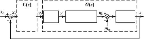
The hydraulic turbine governing system mainly consists of the controller, actuator, hydraulic turbine-conduit and generator-load. The block diagram of hydraulic turbine governing system is shown in Figure 1. From the view in control theory, when the load torque m_g equals to 0, the three parts namely the actuator, hydraulic turbine-conduit and generator-load can be regarded as the controlled object. So the closed-loop HTGS system can be divided into the controller C(s) and the controlled object G(s). Due to the complexity of the system or the changing operation points, there is usually the system model parameter uncertainty. When the hydraulic actuator converts the weak electrical signal to the strong mechanical signal, time-delay occurs in this process. Besides, the fractional order model is more flexible than the integer order model. Thus, considering the terms of fractional order, time-lag and parameter uncertainty, the controlled object can be defined as: (1) $G(s)=\frac{N(s)}{D(s)}=\frac{b_n{s}^{{\beta }_n}+b_{n-1}{s}^{{\beta }_{n-1}}+\cdot \cdot \cdot +b_1{s}^{{\beta }_1}+b_0}{a_n{s}^{{\alpha }_n}+a_{n-1}{s}^{{\alpha }_{n-1}}+\cdot \cdot \cdot +a_1{s}^{{\alpha }_1}+a_0}{e}^{-ls}$(1) where $a_r\in [\underset{\_}{a_r},\overline{a_r}]$ and $b_r\in [\underset{\_}{b_r},\overline{b_r}]$ (r = 0,1,2, … ,n) indicate the transfer function coefficients. $\underset{\_}{a_r}$ and $\overline{a_r}$ are respectively the lower limit and the upper limit of the interval parameters a_r. $\underset{\_}{b_r}$ and $\overline{b_r}$ are respectively the lower limit and the upper limit of the interval parameters b_r. α_r and β_r (0<α₁≤ 1, 1<α₂≤ 2, … , n-1<α_n≤ n; 0<β₁≤ 1, 1<β₂≤ 2, … , n-1<β_n≤ n) are the orders. $l\in [\overline{l},\underset{\_}{l}]$(l > 0) indicates the constant of time-delay. a_r, b_r, α_r and β_r are the arbitrary real numbers. x_c is the given turbine speed and x is the turbine speed. y_c is the output signal of controller and y is the guide vane opening. m_g indicates the load torque and m_t is the turbine torque.

Figure 1. The block diagram of hydraulic turbine governing system.

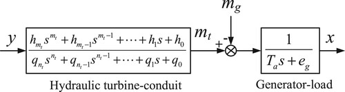
The hydraulic turbine governing system is a closed-loop regulation system which is integrated with water, mechanical and electricity. When the turbine speed changes, the controller changes the control signal to drive open or close the guide vane. These actions make the water flow in the pipes increase or decrease and this can cause the occurrence of water hammer. Therefore, the hydraulic turbine regulation process is a complicated and nonlinear process. To strike a balance between the identification convenience and the model accuracy, the piecewise linear model is used as an approximation to the nonlinear system. The hydraulic turbine-conduit model is partially linear near an operating point and it can be represented by the transfer function model. The model parameters change along with the operating point. The block diagram of hydraulic turbine-conduit and generator-load is shown in Figure 2. q_i and h_j (i = 0,1,2, … ,n_t; j = 0,1,2, … ,m_t; m_t≤ n_t) are the transfer function coefficients. T_a indicates the inertia time constant of generator. e_g is the adjusting coefficient of generator.

Figure 2. The block diagram of hydraulic turbine-conduit and generator-load.

Because of the different operating modes and operating conditions, the system modelling and parameter identification need to be presented respectively for the isolated grid, small grid and no-load operations. In this paper, taking the example of no-load operation, the fractional order transfer function model of hydraulic turbine-conduit and generator-load is built. The fractional order transfer function model of the hydraulic turbine at no-load can be expressed as: (2) $G_{fo}(s)=\frac{x(s)}{y(s)}=\frac{B_1{s}^{{\phi }_1}+B_0}{A_2{s}^{{\theta }_2}+A_1{s}^{{\theta }_1}+1}$(2) where A₂, A₁, B₁ and B₀ are the coefficients of transfer function. θ₂, θ₁ and φ₁ are the orders.

The first order transfer function is used as the actuator with considering the time-delay term (Xu et al., 2015). The transfer function of actuator is defined as: (3) $\frac{y(s)}{y_c(s)}=\frac{1}{T_{y}s+1}{e}^{-Ls}$(3) where T_y indicates the major relay connecter response time and L is the delay time constant.

In this text, the PID, FOPID, PID2D and FOPID2D controllers are applied in the HTGS system. The transfer functions of four controllers are expressed as: (4) $\{\begin{array}{l}{C}_{PID}(s)=k_p+{\displaystyle \frac{k_i}{s}}+k_{d}s{C}_{FOPID}(s)=k_p+{\displaystyle \frac{k_i}{s^{\lambda }}}+k_d{s}^{\mu }{C}_{PID2D}(s)=k_p+{\displaystyle \frac{k_i}{s}}+k_{d}s+k_{d2}{s}^2{C}_{FOPID2D}(s)=k_p+{\displaystyle \frac{k_i}{s^{\lambda }}}+k_d{s}^{\mu }+k_{d2}{s}^{2\mu }\end{array}$(4) where k_p, k_i and k_d indicate the proportional gain, integral gain and differential gain respectively. λ and μ are the integral order and differential order respectively. k_d2 is the second order derivative gain.

2.2. Hydraulic turbine fractional order model parameter identification

When the estimated model outputs including guide vane opening and turbine speed are quite close to the measured data, these parameters including A₂, A₁, B₁, B₀, θ₂, θ₁ and φ₁ can be identified in the hydraulic turbine no-load fractional order model. In recent years, popular artificial intelligence based meta-heuristic algorithms have become effective methods for parameter identification. The algorithms need to strike a balance between exploration and exploitation. As one of the traditional algorithms, the particle swarm optimization algorithm (PSO) has the advantage of few parameters, a simple structure and easy realization. It has a faster convergence speed and higher efficiency than the genetic algorithm. In recent years, the particle swarm optimization algorithm has been applied in different fields and concerned by researchers. Therefore, the particle swarm optimization algorithm is introduced in the parameter identification of the hydraulic turbine fractional order model. η  = [A₂ A₁ B₁ B₀ θ₂ θ₁ φ₁] is the estimated parameter set. Its upper and lower limits of optimization range are [50 50 50 50 2 1 1] and [0 0 -50 0 1 0 0]. The simulation time is 40s and the sample time is 0.005s. For PSO, the population number is 200 and the maximum iteration is 50. The learning factors are set as c₁= c₂= 2. The squared sum of differences between the guide vane opening and turbine speed is set as the fitness function. It can be defined as: (5) $Fit=\sum _{m=1}^{m=M}{(x(m)-\hat{x}(m))}^2+100\cdot \sum _{m=1}^{m=M}{(y(m)-\hat{y}(m))}^2$(5) where M indicates the number of sampling points (m = 1, … ,M). $\hat{y}$ and $\hat{x}$ are the estimated data of guide vane opening and turbine speed respectively. y and x indicate the measured data of guide vane opening and turbine speed.

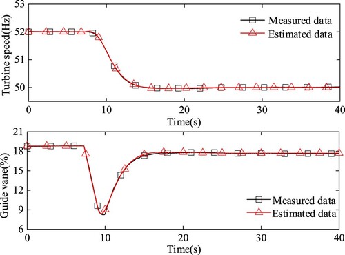
The convergence process of PSO algorithm is shown in Figure 3. The measured and estimated curves of turbine speed and guide vane are compared in Figure 4. The results of turbine speed and guide vane curves in the figures show that the output curves of the estimated model are close to the measured curves. The identified turbine fractional order transfer function model is as follows: (6) $G_{fo}(s)=\frac{x(s)}{y(s)}=\frac{-1.54s^{0.99}+3.93}{33.73s^{1.16}+6.89s^{0.72}+1}$(6)

Figure 3. The iterative convergence process of PSO.

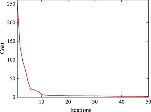
Figure 4. Measured data and estimated data of turbine speed and guide vane.

3. Stability region analysis of FOPID2D controller parameter for hydraulic turbine fractional order interval parameter time-delay system

In this section, the hydraulic turbine fractional order interval parameter time-delay system is separated into several specific parameter subsets by the edge theory. Then the system stability region can be drawn using D-decomposition. The controller parameter values can be obtained when the system stability region maximum is reached. The intersection of stability regions of different parameter subsets is the final system stability region. The present paper briefly introduces the D-decomposition theory and the details can be referred to in the following documents (Hamamic, 2007; Tan, 2005).

In the D-decomposition theory, the imaginary axis of the complex plane is used as a decision boundary and the curve of characteristic polynomial parameters needs to be drawn (Hamamci, 2008). The curve divides the parameter space into stable and unstable regions. Let the characteristic polynomial f(s,a,b) = 0 and put s = jω into the polynomial. Then the curve equation F(a,b) = 0 can be received. Each point (a,b) corresponds to a characteristic equation and this equation has at least one root on the imaginary axis. Considering that the ω has different values, there are three cases of root: the origin root (ω = 0), the infinity pure imaginary root (ω = ∞) and the finite pure imaginary root (0<ω<+∞). At last, the equations of the parameter curve boundary can be solved. Due to space limitations, the stability regions of FOPID2D controller are analysed below. And the stability analysis procedure of FOPID controller is similar to FOPID2D.

The transfer function of close loop system in Figure 1 is as follows: (7) $\frac{x(s)}{x_c(s)}=\frac{C(s)G(s)}{1+C(s)G(s)}$(7) The transfer function of FOPID controller in Equation (2) and the transfer function of controlled object in Equation (1) are brought into Equation (7). The transfer function of the close loop system can be given by: (8) $\begin{array}{rl}\frac{x(s)}{x_c(s)}& =\frac{C_{FOPID}(s)G(s)}{1+C_{FOPID}(s)G(s)}\\ & =\frac{(k_p+k_i/s^{\lambda }+k_d{s}^{\mu })N(s)/D(s)}{1+(k_p+k_i/s^{\lambda }+k_d{s}^{\mu })N(s)/D(s)}\\ & =\frac{(k_p{s}^{\lambda }+k_i+k_d{s}^{\mu +\lambda })N(s)}{D(s)s^{\lambda }+(k_p{s}^{\lambda }+k_i+k_d{s}^{\mu +\lambda })N(s)}\end{array}$(8) The last-written denominator is the characteristic polynomial and it can be expressed as: (9) $\begin{array}{rl}& P(s;k_p,k_i,k_d,k_{d2},\lambda ,\mu )=D(s)s^{\lambda }+(k_p{s}^{\lambda }+k_i+k_d{s}^{\mu +\lambda }\\ & +k_{d2}{s}^{2\mu +\lambda })N(s)\end{array}$(9) where P(s; k_p, k_i, k_d, k_d2, λ, μ) is the characteristic polynomial. It is the denominator of the transfer function of the close loop system in Equation (7).

It is difficult to obtain accurate model and parameters due to the complexity of the actual control system. The system parameters vary with the operating points. Thus, the system parameters remain uncertain. The upper and lower bounds in Equation (10) are used to describe that the parameters may change in the small ranges. The numerator and denominator in Equation (1) can be expressed as: (10) $\{\begin{array}{l}N(s)=\sum _{r=0}^n[\underset{\_}{b_r},\overline{b_r}]s^{{\beta }_r}{e}^{-[\underset{\_}{L},\overline{L}]s}\\ D(s)=\sum _{r=0}^n[\underset{\_}{a_r},\overline{a_r}]s^{{\alpha }_r}\end{array}$(10)

According to the edge theory, under the assumption of n + 2 interval parameters of N(s) and n + 1 interval parameters of D(s), the 2^n + 2 polynomials N^k(s)(k = 1,2, … , 2^n + 2) and 2^n + 1 polynomials D^l(s)(l = 1,2, … ,2^n + 1) can be obtained. If n = 1, the 8 polynomials N^k(s)(k = 1,2, … ,8) and 4 polynomials D^l(s)(l = 1,2, … ,4) can be given as: (11) $\{\begin{array}{l}{N}^1(s)\text{ = (}\overline{b_1}{s}^{{\beta }_1}+\overline{b_0}{s}^{{\beta }_0})e^{-\overline{L}s}\\ ⋮\\ N^8(s)\text{ = (}\underset{\_}{b_1}{s}^{{\beta }_1}+\underset{\_}{b_0}{s}^{{\beta }_0})e^{-\underset{\_}{L}s}\\ D^1(s)\text{ = }\overline{a_0}{s}^{{\alpha }_0}+\overline{a_1}{s}^{{\alpha }_1}\\ ⋮\\ D^4(s)\text{ = }\underset{\_}{a_0}{s}^{{\alpha }_0}+\underset{\_}{a_1}{s}^{{\alpha }_1}\end{array}$(11)

Combining N(s) with D(s), the 2^2n + 3 sub-controlled objects are expressed as: (12) $\begin{array}{rl}G(s)& =\{G_{kl}(s)|G_{kl}(s)=\frac{N^k(s)}{D^l(s)}(k=1,2,\cdots ,2^{n+2};\\ & \times l=1,2,\cdots ,2^{n+1})\phantom{\frac{N^k(s)}{D^l(s)}}\}\end{array}$(12)

From Equation (10) to Equation (9), the closed-loop system characteristic polynomial can be defined as: (13) $\begin{array}{rl}& P(s;k_p,k_i,k_d,k_{d2},\lambda ,\mu )=\sum _{r=0}^n[\underset{\_}{a_r},\overline{a_r}]s^{{\alpha }_r+\lambda }\\ & +(k_p{s}^{\lambda }+k_i+k_d{s}^{\mu +\lambda }+k_{d2}{s}^{2\mu +\lambda })\\ & \times \sum _{r=0}^n{e}^{-[\underset{\_}{L},\overline{L}]s}[\underset{\_}{b_r},\overline{b_r}]s^{{\beta }_r}\end{array}$(13)

The characteristic polynomial of each specific parameter subset can be represented as: (14) $\begin{array}{rl}& P_{kl}(s;k_p,k_i,k_d,k_{d2},\lambda ,\mu )\\ & =D^l(s)s^{\lambda }+e^{-Ls}(k_p{s}^{\lambda }+k_i+k_d{s}^{\mu +\lambda }+k_{d2}{s}^{2\mu +\lambda })N^k(s)\\ & =\sum _{r=0}^n\widehat{a_r}{s}^{{\alpha }_r+\lambda }+(k_p{s}^{\lambda }+k_i+k_d{s}^{\mu +\lambda }+k_{d2}{s}^{2\mu +\lambda })\\ & \times \sum _{r=0}^n{e}^{-\hat{L}s}\widehat{b_r}{s}^{{\beta }_r}\end{array}$(14) where $\widehat{a_r},\widehat{b_r}$ and $\hat{L}$ are the parameter values of the current subset.

It can be seen from Equation (14) that the system stability is influenced by the controller parameters. Thus, it is necessary to gain the parameter space stability region S_kl(C(s)G_kl(s)) of characteristic equation P_kl(s; k_p, k_i, k_d, k_d2, λ, μ). The stability region S_kl(C(s)G_kl(s))∈Ψ is a region of controller parameter space and it can be given as: (15) $\begin{array}{rl}\mathrm{\Psi }& =\{(k_p,k_i,k_d,k_{d2},\lambda ,\mu ):k_p\in [0,\mathrm{\infty }),k_i\in [0,\mathrm{\infty }),\\ & k_d\in [0,\mathrm{\infty }),k_{d2}\in [0,\mathrm{\infty }),\lambda \in [0,2],\mu \in [0,2]\}\end{array}$(15)

With the D-decomposition theory, the different stability regions of G(s) parameter subsets can be established. The parameter space constructed by the FOPID2D controller parameter k_p, k_i, k_d, k_d2, λ and μ contains the points which make the characteristic equation of each parameter set stable. The controller parameter domain can be given by: (16) $\begin{array}{rl}S(C(s)G(s))& =S_{11}(C(s)G_{11}(s))\cap S_{12}(C(s)G_{12}(s))\\ & \cdots S_{kl}(C(s)G_{kl}(s))\end{array}$(16) where k = 1, … ,2^n + 2, l = 1, … ,2^n + 1.

Put s = jω into Equation (14) and the following equation can be expressed as: (17) $\begin{array}{rl}& P_{kl}(j\omega ;k_p,k_i,k_d,\lambda ,\mu )\\ & =\sum _{r=0}^n\widehat{a_r}(j\omega {)}^{{\alpha }_r+\lambda }+(k_p(j\omega {)}^{\lambda }+k_i+k_d(j\omega {)}^{\mu +\lambda }\\ & +k_{d2}(j\omega {)}^{2\mu +\lambda })\sum _{r=0}^n{e}^{-\hat{L}j\omega }\widehat{b_r}{(j\omega )}^{{\beta }_r}\end{array}$(17)

The parameter boundary curves can be got through the D-decomposition theory. Take ω = 0 into Equation (17) and let P_kl = 0. The following equation can be given by: (18) $P_{kl}(0;k_p,k_i,k_d,k_{d2},\lambda ,\mu )=\widehat{b_r}{k}_i=0\iff k_i=0$(18) where $s^{{\beta }_0}=1$ is established in each parameter set transfer function of Equation (18), thus β₀= 0.

When the condition α_n≤β_n+ 2μ is met, the boundary curves of infinite pure imaginary roots exist. It can be described as: (19) $\{\begin{array}{ll}{k}_{d2}=0& \begin{array}{l}({\alpha }_n={\beta }_n)or({\alpha }_n>{\beta }_n\text{and}\mu >1/2({\alpha }_n-{\beta }_n))\end{array}\\ k_{d2}=\pm a_n/b_n& \begin{array}{l}({\alpha }_n>{\beta }_{n}and\\ \mu =1/2({\alpha }_n-{\beta }_n))\end{array}\\ none& \begin{array}{l}({\alpha }_n>{\beta }_{n}and\\ \mu <1/2({\alpha }_n-{\beta }_n))\end{array}\end{array}$(19)

Then Equation (17) can be presented as: (20) $\begin{array}{rl}& P_{kl}(j\omega ;k_p,k_i,k_d,\lambda ,\mu )\\ & =\sum _{r=0}^n\widehat{a_r}(j\omega {)}^{\widehat{{\alpha }_r}}+(k_p+k_i(j\omega {)}^{-\lambda }+k_d(j\omega {)}^{\mu }\\ & +k_{d2}(j\omega {)}^{2\mu })\sum _{r=0}^n{e}^{-j\hat{L}\omega }\\ & =\sum _{r=0}^n\widehat{a_r}(j\omega {)}^{\widehat{{\alpha }_r}}+e^{-j\hat{L}\omega }\widehat{b_r}[k_p+k_i(j\omega {)}^{\widehat{{\beta }_r}-\lambda }\\ & +k_d(j\omega {)}^{\widehat{{\beta }_r}+\mu }+k_{d2}(j\omega {)}^{\widehat{{\beta }_r}+2\mu }]\\ & =0\end{array}$(20)

The non-integer order of complex numbers can be expressed as: (21) $\begin{array}{rl}(\sigma +j\rho {)}^{\delta }& =\sqrt[\delta ]{{\sigma }^2+{\rho }^2}[cos\left(\delta ta{n}^{-1}\left(\frac{\rho }{\sigma }\right)\right)\\ & +j\sin \left(\delta ta{n}^{-1}\left(\frac{\rho }{\sigma }\right)\right)]\end{array}$(21)

With the Euler equation, the terms in Equation (20) can be given as: (22) $\begin{array}{rl}{e}^{j\varphi }& =\cos \varphi +j\sin \varphi \end{array}$(22) (23) $\begin{array}{rl}{j}^{{\alpha }_r}& =\cos \left(\frac{\pi }{2}{\alpha }_r\right)+j\sin \left(\frac{\pi }{2}{\alpha }_r\right)=x_r+j{y}_r\end{array}$(23) (24) $\begin{array}{rl}{j}^{{\beta }_r}& =\cos \left(\frac{\pi }{2}{\beta }_r\right)+j\sin \left(\frac{\pi }{2}{\beta }_r\right)=z_r+j{t}_r\end{array}$(24) (25) $\begin{array}{rl}{j}^{{\beta }_r-\lambda }& =\cos (\frac{\pi }{2}({\beta }_r-\lambda ))+j\sin (\frac{\pi }{2}({\beta }_r-\lambda ))=q_r+j{h}_r\end{array}$(25) (26) $\begin{array}{rl}{j}^{{\beta }_r+\mu }& =\cos (\frac{\pi }{2}({\beta }_r+\mu ))+j\sin (\frac{\pi }{2}({\beta }_r+\mu ))\\ & =m_r+j{k}_r\end{array}$(26) (27) $\begin{array}{rl}{e^{-j}}^{\hat{L}\omega }& =\cos (-\hat{L}\omega )+j\sin (-\hat{L}\omega )=cos(\hat{L}\omega )-j\sin (\hat{L}\omega )\end{array}$(27) (28) $\begin{array}{rl}{j}^{{\beta }_r+2\mu }& =\cos (\frac{\pi }{2}(\widehat{{\beta }_r}+2\mu ))+j\sin (\frac{\pi }{2}(\widehat{{\beta }_r}+2\mu ))\\ & =n_r+j{f}_r\end{array}$(28)

Thus, the Equation (20) can be expressed as: (29) $\begin{array}{rl}& P_{kl}(j\omega ;k_p,k_i,k_d,k_{d2},\lambda ,\mu )\\ & =\sum _{r=0}^n\widehat{a_r}{\omega }^{\widehat{{\alpha }_r}}(x_r+j{y}_r)+\widehat{b_r}(cos(\hat{L}\omega )\\ & -j\sin (\hat{L}\omega ))[k_p{\omega }^{\widehat{{\beta }_r}}(z_r+j{t}_r)\\ & +k_i{\omega }^{\widehat{{\beta }_r}-\lambda }(q_r+j{h}_r)+k_d{\omega }^{\widehat{{\beta }_r}+\mu }(m_r+j{k}_r)\\ & +k_{d2}{\omega }^{\widehat{{\beta }_r}+2\mu }(n_r+j{f}_r)]\\ & =Re(P_{kl}(j\omega ;k_p,k_i,k_d,k_{d2},\lambda ,\mu ))\\ & +j\mathrm{Im}(P_{kl}(j\omega ;k_p,k_i,k_d,k_{d2},\lambda ,\mu ))\\ & =0\end{array}$(29)

Let the values of the real part and the imaginary part equal to 0 respectively. The following equations can be obtained: (30) $\{\begin{array}{c}{k}_{p}M(\omega )+k_{i}N(\omega )=k_{d}B(\omega )+k_{d2}K(\omega )+X(\omega )\\ k_{p}A(\omega )+k_{i}H(\omega )=k_{d}Z(\omega )+k_{d2}T(\omega )+Y(\omega )\end{array}$(30) where: (31) $\begin{array}{rl}& \{\begin{array}{l}M(\omega )=\cos (\hat{L}\omega )\sum _{r=0}^n\widehat{b_r}{z}_r{\omega }^{{\beta }_r}+\sin (\hat{L}\omega )\sum _{r=0}^n\widehat{b_r}{t}_r{\omega }^{{\beta }_r}\\ N(\omega )=\cos (\hat{L}\omega )\sum _{r=0}^n\widehat{b_r}{q}_r{\omega }^{{\beta }_r-\lambda }+\sin (\hat{L}\omega )\sum _{r=0}^n\widehat{b_r}{t}_r{\omega }^{{\beta }_r-\lambda }\\ B(\omega )=-\cos (\hat{L}\omega )\sum _{r=0}^n\widehat{b_r}{m}_r{\omega }^{{\beta }_r+\mu }-\sin (\hat{L}\omega )\sum _{r=0}^n\widehat{b_r}{k}_r{\omega }^{{\beta }_r+\mu }\\ X(\omega )=-\sum _{r=0}^n\widehat{a_r}{x}_r{\omega }^{{\alpha }_r}\\ K(\omega )=-\cos (\hat{L}\omega )\sum _{r=0}^n\widehat{b_r}{m}_r{\omega }^{\widehat{{\beta }_r}+2\mu }-\sin (\hat{L}\omega )\sum _{r=0}^n\widehat{b_r}{k}_r{\omega }^{\widehat{{\beta }_r}+2\mu }\end{array}\end{array}$(31) (32) $\begin{array}{rl}& \{\begin{array}{l}A(\omega )=\cos (\hat{L}\omega )\sum _{r=0}^n\widehat{b_r}{t}_r{\omega }^{{\beta }_r}-\sin (\hat{L}\omega )\sum _{r=0}^n\widehat{b_r}{z}_r{\omega }^{{\beta }_r}\\ H(\omega )=\cos (\hat{L}\omega )\sum _{r=0}^n\widehat{b_r}{h}_r{\omega }^{{\beta }_r-\lambda }+\sin (\hat{L}\omega )\sum _{r=0}^n\widehat{b_r}{q}_r{\omega }^{{\beta }_r-\lambda }\\ Z(\omega )=\sin (\hat{L}\omega )\sum _{r=0}^n\widehat{b_r}{m}_r{\omega }^{{\beta }_r+\mu }-\cos (\hat{L}\omega )\sum _{r=0}^n\widehat{b_r}{k}_r{\omega }^{{\beta }_r+\mu }\\ Y(\omega )=-\sum _{r=0}^n\widehat{a_r}{y}_r{\omega }^{{\alpha }_r}\\ T(\omega )=\sin (\hat{L}\omega )\sum _{r=0}^n\widehat{b_r}{m}_r{\omega }^{\widehat{{\beta }_r}+2\mu }-\cos (\hat{L}\omega )\sum _{r=0}^n\widehat{b_r}{k}_r{\omega }^{\widehat{{\beta }_r}+2\mu }\end{array}\end{array}$(32)

From Equation (32), the parameters k_p and k_i which depend on the parameters k_d, λ and μ for FOPID2D controller can be given as: (33) $\{\begin{array}{l}{k}_p={\displaystyle \frac{\begin{array}{c}X\cdot H-Y\cdot N+k_d(B\cdot H-Z\cdot N)\\ +k_{d2}(K\cdot H-T\cdot N)\end{array}}{M\cdot H-A\cdot N}}{k}_i={\displaystyle \frac{\begin{array}{c}X\cdot A-Y\cdot M+k_d(B\cdot A-Z\cdot M)\\ +k_{d2}(K\cdot A-T\cdot M)\end{array}}{A\cdot N-M\cdot H}}\end{array}$(33)

Similarly, through the theoretical deduction, the parameters k_p and k_i which depend on the parameters k_d, λ and μ for FOPID controller can be expressed as: (34) $\{\begin{array}{l}{k}_p={\displaystyle \frac{X\cdot H-Y\cdot N+k_d(B\cdot H-Z\cdot N)}{M\cdot H-A\cdot N}}{k}_i={\displaystyle \frac{X\cdot A-Y\cdot M+k_d(B\cdot A-Z\cdot M)}{A\cdot N-M\cdot H}}\end{array}$(34)

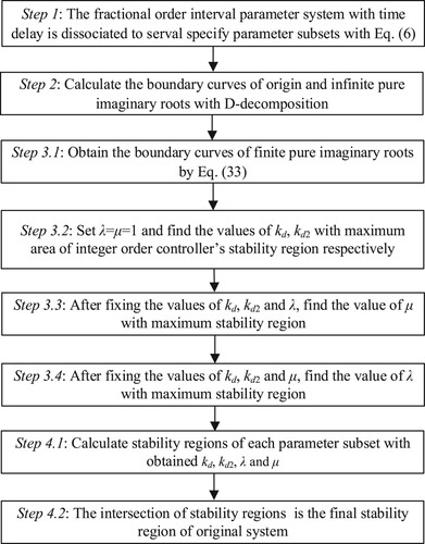
It can be known from Equation (33) that k_d, k_d2, λ and μ are the independent variables and k_p and k_i are the dependent variables. If k_d, k_d2, λ and μ have fixed values and ω increases from 0 to ∞, the boundary curve of finite pure imaginary root can be drawn in the two dimensional plane (k_p, k_i). Similarly, the correlation equations in which the FOPID2D controller parameters such as k_p, k_d or k_i, k_d or k_i, k_d2 depend on the other parameters observed by solving the Equation (33). Byfixing the value of independent variables, the boundary curves of the finite pure imaginary root can be obtained. Because of space limitations, the paper only presents the boundary curves of finite pure imaginary root in the plane (k_p, k_i). In addition, the controller parameters of the system are usually real numbers while drawing the stability regions. Finally, the stability region of FOPID2D controller parameter in the hydraulic turbine fractional order interval parameter time-delay system is computed and analysed. Figure 5 shows the calculation steps of the stability region of FOPID2D controller parameter.

Figure 5. Calculation steps of stability region of FOPID2D controller parameter.

4. Result and analysis

For the convenience of readers, the main results of this paper should be presented in the form of propositions. These propositions are shown as follows:

Proposition 1:

The stability comparison of different controllers for the hydraulic turbine fractional order interval parameter time-delay system shows that FOPID2D has the biggest stability region, FOPID is moderate, PID2D takes the third place and PID is the least. The FOPID2D controller has better robust stability than the others.

Proposition 2:

The variable laws of stability regions of FOPID2D, PID2D, FOPID and PID controller parameters for the hydraulic turbine fractional order interval parameter time-delay system are as follows:

1. The system stability region first decreases and then increases with λ decreasing from 1.6 to 0.2.

2. The system stability region first increases and then decreases with μ decreasing from 1.9 to 0.3.

3. The system stability region decreases with k_d2 decreasing from 1 to 0.2.

4. The system stability region decreases with k_d decreasing from 1 to 0.2.

The transfer function model of the controlled object in the hydraulic turbine governing system can be given by: (35) $\begin{array}{rl}G(s)& =\frac{1}{T_{y}s+1}\cdot \frac{B_1{s}^{{\phi }_1}+B_0}{A_2{s}^{{\theta }_2}+A_1{s}^{{\theta }_1}+1}{e}^{-Ls}\\ & =\frac{B_1{s}^{{\phi }_1}+B_0}{\begin{array}{c}{T}_y{A}_2{s}^{{\theta }_2+1}+T_y{A}_1{s}^{{\theta }_1+1}+T_{y}s\\ +A_2{s}^{{\theta }_2}+A_1{s}^{{\theta }_1}+1\end{array}}{e}^{-Ls}\end{array}$(35)

In the established hydraulic turbine governing system, the controlled object parameters can be selected as the uncertain parameters. For the actuator, the major relay connecter response time T_y can be obtained through the signal practical experiments. Considering the hydraulic turbine parameters changing along with the operating points and the uncertain error of delay time, the fractional order transfer function coefficients and the time-delay are set as the interval parameters. In order to facilitate the realization of the simulation result display, it is assumed that the parameter uncertainties come from the parameters A₂, B₀ and L. Set the nominal values of these parameters: A₂= 33.73, A₁= 6.89, B₁= −1.54, B₀= 3.93, θ₂= 1.16, θ₁= 0.72, φ₁= 0.99, T_y= 0.1, L = 1.25. The interval parameters A₂, B₀ and L are considered to vary in the range of 20%, 10% and 10% respectively. Thus, $A_2\in [\underset{\_}{A_2},\overline{A_2}]$ = [26.98, 40.48], $B_0\in [\underset{\_}{B_0},\overline{B_0}]$  = [3.54, 4.32], $L\in [\underset{\_}{L},\overline{L}]$ = [1.13, 1.38]. With the D-decomposition theory, there are eight models of parameter subsets. They can be expressed as: (36) $\{\begin{array}{l}{G}_{11}(s)={\displaystyle \frac{B_1{s}^{{\phi }_1}+\underset{\_}{B_0}}{\begin{array}{c}{T}_y\underset{\_}{A_2}{s}^{{\theta }_2+1}+T_y{A}_1{s}^{{\theta }_1+1}+T_{y}s\\ +\underset{\_}{A_2}{s}^{{\theta }_2}+A_1{s}^{{\theta }_1}+1\end{array}}}{e}^{-\underset{\_}{L}s}{G}_{12}(s)={\displaystyle \frac{B_1{s}^{{\phi }_1}+\overline{B_0}}{\begin{array}{c}{T}_y\underset{\_}{A_2}{s}^{{\theta }_2+1}+T_y{A}_1{s}^{{\theta }_1+1}+T_{y}s\\ +\underset{\_}{A_2}{s}^{{\theta }_2}+A_1{s}^{{\theta }_1}+1\end{array}}}{e}^{-\underset{\_}{L}s}{G}_{13}(s)={\displaystyle \frac{B_1{s}^{{\phi }_1}+\underset{\_}{B_0}}{\begin{array}{c}{T}_y\overline{A_2}{s}^{{\theta }_2+1}+T_y{A}_1{s}^{{\theta }_1+1}+T_{y}s\\ +\overline{A_2}{s}^{{\theta }_2}+A_1{s}^{{\theta }_1}+1\end{array}}}{e}^{-\underset{\_}{L}s}{G}_{14}(s)={\displaystyle \frac{B_1{s}^{{\phi }_1}+\overline{B_0}}{\begin{array}{c}{T}_y\overline{A_2}{s}^{{\theta }_2+1}+T_y{A}_1{s}^{{\theta }_1+1}+T_{y}s\\ +\overline{A_2}{s}^{{\theta }_2}+A_1{s}^{{\theta }_1}+1\end{array}}}{e}^{-\underset{\_}{L}s}{G}_{21}(s)={\displaystyle \frac{B_1{s}^{{\phi }_1}+\underset{\_}{B_0}}{\begin{array}{c}{T}_y\underset{\_}{A_2}{s}^{{\theta }_2+1}+T_y{A}_1{s}^{{\theta }_1+1}+T_{y}s\\ +\underset{\_}{A_2}{s}^{{\theta }_2}+A_1{s}^{{\theta }_1}+1\end{array}}}{e}^{-\overline{L}s}{G}_{22}(s)={\displaystyle \frac{B_1{s}^{{\phi }_1}+\overline{B_0}}{\begin{array}{c}{T}_y\underset{\_}{A_2}{s}^{{\theta }_2+1}+T_y{A}_1{s}^{{\theta }_1+1}+T_{y}s\\ +\underset{\_}{A_2}{s}^{{\theta }_2}+A_1{s}^{{\theta }_1}+1\end{array}}}{e}^{-\overline{L}s}{G}_{23}(s)={\displaystyle \frac{B_1{s}^{{\phi }_1}+\underset{\_}{B_0}}{\begin{array}{c}{T}_y\overline{A_2}{s}^{{\theta }_2+1}+T_y{A}_1{s}^{{\theta }_1+1}+T_{y}s\\ +\overline{A_2}{s}^{{\theta }_2}+A_1{s}^{{\theta }_1}+1\end{array}}}{e}^{-\overline{L}s}{G}_{24}(s)={\displaystyle \frac{B_1{s}^{{\phi }_1}+\overline{B_0}}{\begin{array}{c}{T}_y\overline{A_2}{s}^{{\theta }_2+1}+T_y{A}_1{s}^{{\theta }_1+1}+T_{y}s\\ +\overline{A_2}{s}^{{\theta }_2}+A_1{s}^{{\theta }_1}+1\end{array}}}{e}^{-\overline{L}s}\end{array}$(36)

4.1. Stability region results of PID and FOPID controllers

The characteristic function of the hydraulic turbine fractional order model based on FOPID controller can be given by: (37) $\begin{array}{rl}& P(s;k_p,k_i,k_d,\lambda ,\mu )\\ & =T_y\widehat{A_2}{s}^{{\theta }_2+1+\lambda }+T_y{A}_1{s}^{{\theta }_1+1+\lambda }+T_y{s}^{1+\lambda }\\ & +\widehat{A_2}{s}^{{\theta }_2+\lambda }+A_1{s}^{{\theta }_1+\lambda }+s^{\lambda }\\ & +e^{-\hat{L}s}(B_1{s}^{{\phi }_1}+\widehat{B_0})(k_p{s}^{\lambda }+k_i+k_d{s}^{\mu +\lambda })\end{array}$(37) where $\widehat{A_2}$, $\widehat{B_0}$ and $\hat{L}$ indicate the interval parameters.

With the D-decomposition theory, the boundary curves of origin (ω = 0) and infinite (ω = ∞) pure imaginary roots can be calculated as: (38) $\begin{array}{rl}& \text{Origin}{k}_i=0\text{Because}{s}^{{\beta }_0}=1\end{array}$(38) (39) $\begin{array}{rl}& \text{Infinite pure imaginary root}\text{:}\{\begin{array}{llll}{k}_d=0& (\mu >1.17)k_d=\pm {\displaystyle \frac{T_y\widehat{A_2}}{B_1}}& (\mu =1.17)none& (\mu <1.17)\end{array}\end{array}$(39) From Equations (31) and (32), the boundary curves of finite (0<ω<+∞) pure imaginary root can be given: (40) $\begin{array}{rl}& \{\begin{array}{rl}M& =cos(L\omega )(B_1{\omega }^{{\phi }_1}cos\left({\displaystyle \frac{\pi }{2}}{\phi }_1\right)+B_0)\\ & +sin(L\omega )\sin \left({\displaystyle \frac{\pi }{2}}{\phi }_1\right)B_1{\omega }^{{\phi }_1}\\ N& ={\omega }^{-\lambda }\cos \left({\displaystyle \frac{\pi }{2}}\lambda \right)[cos(L\omega )(B_1{\omega }^{{\phi }_1}cos\left({\displaystyle \frac{\pi }{2}}{\phi }_1\right)+B_0)\\ & +sin(L\omega )\sin \left({\displaystyle \frac{\pi }{2}}{\phi }_1\right)B_1{\omega }^{{\phi }_1}]+{\omega }^{-\lambda }\sin \left({\displaystyle \frac{\pi }{2}}\lambda \right)\\ & [-sin(L\omega )(B_1{\omega }^{{\phi }_1}cos\left({\displaystyle \frac{\pi }{2}}{\phi }_1\right)+B_0)\\ & +cos(L\omega )B_1{\omega }^{{\phi }_1}\sin \left({\displaystyle \frac{\pi }{2}}{\phi }_1\right)]\\ B& =-{\omega }^{\mu }\cos \left({\displaystyle \frac{\pi }{2}}\mu \right)[cos(L\omega )(B_1{\omega }^{{\phi }_1}cos\left({\displaystyle \frac{\pi }{2}}{\phi }_1\right)+B_0)\\ & +sin(L\omega )\sin \left({\displaystyle \frac{\pi }{2}}{\phi }_1\right)B_1{\omega }^{{\phi }_1}]+{\omega }^{\mu }\sin \left({\displaystyle \frac{\pi }{2}}\mu \right)\\ & [-sin(L\omega )(B_1{\omega }^{{\phi }_1}cos\left({\displaystyle \frac{\pi }{2}}{\phi }_1\right)+B_0)\\ & +cos(L\omega )B_1{\omega }^{{\phi }_1}\sin \left({\displaystyle \frac{\pi }{2}}{\phi }_1\right)]\\ X& =-T_y{A}_2{\omega }^{{\theta }_2+1}\cos ({\displaystyle \frac{\pi }{2}}({\theta }_2+1))\\ & -T_y{A}_1{\omega }^{{\theta }_1+1}\cos ({\displaystyle \frac{\pi }{2}}({\theta }_1+1))-A_2{\omega }^{{\theta }_2}\cos \left({\displaystyle \frac{\pi }{2}}{\theta }_2\right)\\ & -A_1{\omega }^{{\theta }_1}\cos \left({\displaystyle \frac{\pi }{2}}{\theta }_1\right)\end{array}\end{array}$(40) (41) $\begin{array}{rl}& \{\begin{array}{rlrlrlrlrlrllllll}A& =-sin(L\omega )(B_1{\omega }^{{\phi }_1}cos\left({\displaystyle \frac{\pi }{2}}{\phi }_1\right)+B_0)& +cos(L\omega )B_1{\omega }^{{\phi }_1}\sin \left({\displaystyle \frac{\pi }{2}}{\phi }_1\right)H& =-{\omega }^{-\lambda }sin(L\omega )[cos(L\omega )(b_1{\omega }^{{\phi }_1}cos\left({\displaystyle \frac{\pi }{2}}{\phi }_1\right)+B_0)& -sin(L\omega )\sin \left({\displaystyle \frac{\pi }{2}}{\beta }_1\right)B_1{\omega }^{{\phi }_1}]& +{\omega }^{-\lambda }\cos \left({\displaystyle \frac{\pi }{2}}\lambda \right)& [-sin(L\omega )(B_1{\omega }^{{\phi }_1}cos\left({\displaystyle \frac{\pi }{2}}{\phi }_1\right)+B_0)& +cos(L\omega )B_1{\omega }^{{\phi }_1}\sin \left({\displaystyle \frac{\pi }{2}}{\phi }_1\right)]Z& =-{\omega }^{\mu }sin\left({\displaystyle \frac{\pi }{2}}\mu \right)[cos(L\omega )(B_1{\omega }^{{\phi }_1}cos\left({\displaystyle \frac{\pi }{2}}{\phi }_1\right)+B_0)& -sin(L\omega )\sin \left({\displaystyle \frac{\pi }{2}}{\phi }_1\right)B_1{\omega }^{{\phi }_1}]& -{\omega }^{\mu }sin\left({\displaystyle \frac{\pi }{2}}\mu \right)& [-sin(L\omega )(b_1{\omega }^{{\phi }_1}cos\left({\displaystyle \frac{\pi }{2}}{\phi }_1\right)+B_0)& +cos(L\omega )B_1{\omega }^{{\phi }_1}\sin \left({\displaystyle \frac{\pi }{2}}{\phi }_1\right)]Y& =-T_y{A}_2{\omega }^{{\theta }_2+1}sin({\displaystyle \frac{\pi }{2}}({\theta }_2+1))& -T_y{A}_1{\omega }^{{\theta }_1+1}sin({\displaystyle \frac{\pi }{2}}({\theta }_1+1))& -T_y\omega -A_2{\omega }^{{\theta }_2}sin\left({\displaystyle \frac{\pi }{2}}{\theta }_2\right)& -A_1{\omega }^{{\theta }_1}sin\left({\displaystyle \frac{\pi }{2}}{\theta }_1\right)\end{array}\end{array}$(41)

1. Stability region of PID controller

Because the stability region variation trends of hydraulic turbine fractional order parameter subset models are nearly the same, G₁₃ and G₂₁ are taken as examples. Set λ = μ = 1 and k_d decreases from 1 to 0.2 linearly. Then the boundary curves of finite pure imaginary root can be drawn. The area composed of curves of origin and infinite pure imaginary roots is the stability region. It can be known from Table 1 and Figure 6 that the stability region of PID controller increases with k_d increasing and the area size is largest with k_d  = 1.

Figure 6. Stability regions of G₁₃ and G₂₁ with various k_d values for PID. (a) G₁₃. (b) G₂₁.

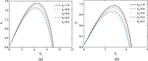
Table 1. Stability region comparison of different k_d values for PID.

Model	kd = 1	kd = 0.8	kd = 0.6	kd = 0.4	kd = 0.2
G13	13.36	12.76	12.16	11.59	11.03
G21	5.23	4.93	4.63	4.34	4.07

As Table 2 and Figure 7 show, set k_d= 1, the stability regions of PID controller parameter sets can be calculated and drawn. The intersection of all parameter sets’ stability regions can be determined. It can be seen from Table 2 that the stability region of G₂₂ model is the smallest among the all models. In Figure 6, the intersection of G₂₁, G₂₂, G₂₃ and G₂₃ models parameter sets’ stability regions is the final stability region. The size of PID parameters’ stability region for the established HTGS system is 4.12 by calculation.

1. Stability region of FOPID controller

Figure 7. Stability regions of all parameter subsets G₁₁-G₂₄ for PID.

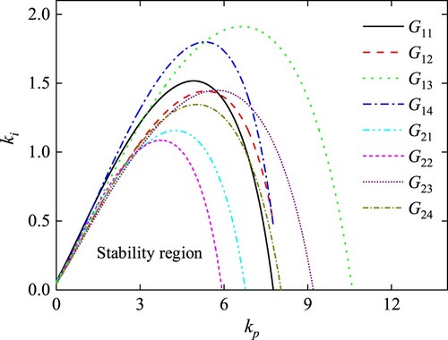
Table 2. Stability region comparison of different parameter subsets for PID.

Parameter subset	G11	G12	G13	G14	G21	G22	G23	G24
Stability region	7.83	6.58	13.36	11.10	5.23	4.29	8.83	7.16

Set k_d= 1 and μ = 1, the value of λ decrease from 1.6 to 0.2 linearly. With the variable values of λ, the boundary curves of FOPID controller can be drawn and the area sizes of stability region can be determined. As shown in Table 3 and Figure 8, when λ<1.4, the area of FOPID controller stability region decreases with λ increasing. When λ>1.4, the area of FOPID controller stability region increases with λ increasing. Therefore, the area size of FOPID controller stability region for the HTGS system is largest with λ = 0.2.

Figure 8. Stability regions of G₁₃ and G₂₁ with various λ values for FOPID. (a) G₁₃. (b) G_21.

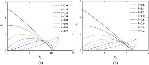
Table 3. Stability region comparison of different λ values for FOPID.

Model	λ=1.6	λ=1.4	λ=1.2	λ=1.0	λ=0.8	λ=0.6	λ=0.4	λ=0.2
G13	10.96	10.16	11.32	13.36	16.99	32.16	32.30	43.71
G21	4.06	3.74	4.30	5.23	6.82	9.42	13.17	17.77

Similarly, set k_d= 1 and λ = 1, the value of μ decrease from 1.9 to 0.3 linearly. As is apparent from Table 4 and Figure 9, when μ<0.9, the area of FOPID controller stability region increases with μ increasing. When μ>0.9, the area of FOPID controller stability region decreases with μ increasing. The area size of FOPID controller stability region is largest with μ = 0.9.

Figure 9. Stability regions of G₁₃ and G₂₁ with various μ values for FOPID. (a) G₁₃. (b) G₂₁.

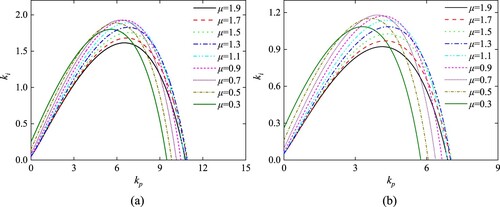
Table 4. Stability region comparison of different μ values for FOPID.

Model	μ = 1.9	μ = 1.7	μ = 1.5	μ = 1.3	μ = 1.1	μ = 0.9	μ = 0.7	μ = 0.5	μ = 0.3
G13	11.48	12.09	12.65	13.08	13.33	13.34	13.11	12.63	11.89
G21	4.25	4.53	4.81	5.05	5.20	5.23	5.13	4.90	4.51

Set k_d= 1, λ = 0.2. and μ = 0.9, the boundary curve of different FOPID controller parameter sets’ stability regions can be drawn. It can be observed from Figure 10 and Table 5 that the area of G₂₂ model’s stability region is the smallest and it is the intersection of whole models’ stability regions. The area size of FOPID controller stability region is 13.41 with the comparison results.

Figure 10. Stability regions of all parameter subsets G₁₁-G₂₄ for FOPID.

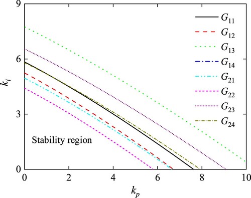
Table 5. Stability region comparison of different parameter subsets for FOPID.

Parameter subset	G11	G12	G13	G14	G21	G22	G23	G24
Stability region	23.39	18.46	42.73	33.64	17.29	13.41	31.35	24.20

4.2. Stability region results of PID2D and FOPID2D controllers

The characteristic function of hydraulic turbine fractional order model based on FOPID2D controller can be given by: (42) $\begin{array}{rl}& P(s;k_p,k_i,k_d,k_{d2},\lambda ,\mu )\\ & =T_y\widehat{A_2}{s}^{{\theta }_2+1+\lambda }+T_y{A}_1{s}^{{\theta }_1+1+\lambda }+T_y{s}^{1+\lambda }+\widehat{A_2}{s}^{{\theta }_2+\lambda }\\ & +A_1{s}^{{\theta }_1+\lambda }+s^{\lambda }+e^{-\hat{L}s}(B_1{s}^{{\phi }_1}+\widehat{B_0})\\ & \times (k_p{s}^{\lambda }+k_i+k_d{s}^{\mu +\lambda }+k_{d2}{s}^{2\mu +\lambda }))\end{array}$(42) where $\widehat{A_2}$, $\widehat{B_0}$ and $\hat{L}$ indicate the interval parameters.

With the D-decomposition theory, the boundary curves of origin (ω = 0) and infinite (ω = ∞) pure imaginary roots can be calculated as: (43) $\begin{array}{rl}& \text{Origin}\text{:}{k}_i=0\text{Because}{s}^{{\beta }_0}=1\end{array}$(43) (44) $\begin{array}{rl}& \text{Infinite pure imaginary root}\text{:}\{\begin{array}{llll}{k}_{d2}=0& (\mu >0.59)k_{d2}=\pm {\displaystyle \frac{T_y\widehat{A_2}}{B_1}}& (\mu =0.59)none& (\mu <0.59)\end{array}\end{array}$(44) From Equations (31) and (32), the boundary curves of finite (0<ω<+∞) pure imaginary root can be given and the coefficient can be expressed in Equation (45): (45) $\{\begin{array}{rlrlrlrlr}K& =-{\omega }^{2\mu }\cos (\pi \mu )[cos(L\omega )(B_1{\omega }^{{\phi }_1}cos\left({\displaystyle \frac{\pi }{2}}{\phi }_1\right)+B_0)& +sin(L\omega )\sin \left({\displaystyle \frac{\pi }{2}}{\phi }_1\right)B_1{\omega }^{{\phi }_1}]& +{\omega }^{2\mu }\sin (\pi \mu )[-sin(L\omega )(B_1{\omega }^{{\phi }_1}cos\left({\displaystyle \frac{\pi }{2}}{\phi }_1\right)+B_0)& +cos(L\omega )B_1{\omega }^{{\phi }_1}\sin \left({\displaystyle \frac{\pi }{2}}{\phi }_1\right)]T& =-{\omega }^{2\mu }sin(\pi \mu )[cos(L\omega )(B_1{\omega }^{{\phi }_1}cos\left({\displaystyle \frac{\pi }{2}}{\phi }_1\right)+B_0)& -sin(L\omega )\sin \left({\displaystyle \frac{\pi }{2}}{\phi }_1\right)B_1{\omega }^{{\phi }_1}]& -{\omega }^{2\mu }sin(\pi \mu )[-sin(L\omega )(B_1{\omega }^{{\phi }_1}cos\left({\displaystyle \frac{\pi }{2}}{\phi }_1\right)+B_0)& +cos(L\omega )B_1{\omega }^{{\phi }_1}\sin \left({\displaystyle \frac{\pi }{2}}{\phi }_1\right)]\end{array}$(45)

1. Stability region of PID2D controller

In Figure 11 and Table 6, set k_d= 1 and λ = μ = 1, the value of k_d2 decrease from 1 to 0.2 linearly. It is clear that the area of PID2D controller stability region increases with k_d2 increasing.

Figure 11. Stability regions of G₁₃ and G₂₁ with various k_d2 values for PID2D. (a) G₁₃. (b) G₂₁.

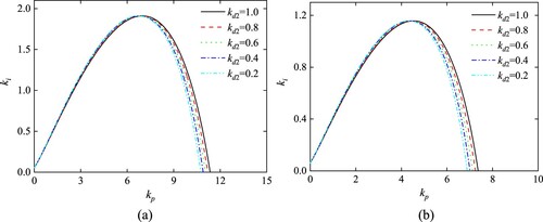
Table 6. Stability region comparison of different k_d2 values for PID2D.

Model	kd2 = 1	kd2 = 0.8	kd2 = 0.6	kd2 = 0.4	kd2 = 0.2
G13	14.31	14.12	13.93	13.74	13.55
G21	5.69	5.60	5.51	5.42	5.32

Similarly, set k_d2= 1 and λ = μ = 1, the value of k_d decrease from 1 to 0.2 linearly. From the results of Figure 12 and Table 7, the area of PID2D controller stability region increases with k_d increasing.

Figure 12. Stability regions of G₁₃ and G₂₁ with various k_d values for PID2D. (a) G₁₃. (b) G₂₁.

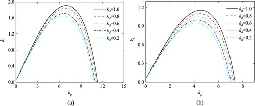
Table 7. Stability region comparison of different k_d values for PID2D.

Model	kd = 1	kd = 0.8	kd = 0.6	kd = 0.4	kd = 0.2
G13	14.31	13.65	13.01	12.38	11.78
G21	5.69	5.35	5.02	4.71	4.40

In this text, k_d= 1 and k_d2= 1 is set. From Table 8 and Figure 13, the area of G₂₂ model’s stability region is the smallest. The intersection of G₂₁, G₂₂, G₂₃ and G₂₃ models’ stability regions is the final stability region. The final area size of PID2D controller stability region for the HTGS system is 4.69.

1. Stability region of FOPID2D controller

Figure 13. Stability regions of all parameter subsets G₁₁-G₂₄ for PID2D.

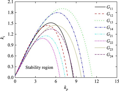
Table 8. Stability region comparison of different parameter subsets for PID2D.

Parameter subset	G11	G12	G13	G14	G21	G22	G23	G24
Stability region	8.63	7.43	14.31	12.10	5.69	4.78	9.37	7.72

Set k_d= 1, k_d2= 1 and μ = 1, the value of λ decrease from 1.6 to 0.2 linearly. Then the stability region of FOPID2D controller can be determined with different values of λ. As can be seen from Table 9 and Figure 14, the system stability region first decreases and then increases with λ decreasing from 1.6 to 0.2. And the area size of FOPID2D controller stability region is largest with λ = 0.2.

Figure 14. Stability regions of G₁₃ and G₂₁ with various λ values for FOPID2D. (a) G₁₃. (b) G₂₁.

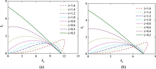
Table 9. Stability region comparison of different λ values for FOPID2D.

Model	λ = 1.6	λ = 1.4	λ = 1.2	λ = 1.0	λ = 0.8	λ = 0.6	λ = 0.4	λ = 0.2
G13	11.52	11.09	12.21	14.31	18.12	24.72	34.93	48.37
G21	4.27	4.16	4.73	5.69	7.38	10.22	14.54	20.32

Similarly, set k_d= 1, k_d2= 1 and λ = 1, the value of μ decrease from 1.9 to 0.3 linearly. As is clear from Table 10 and Figure 15, when μ>0.7, the area of stability region increases with μ decreasing. When μ<0.7, the area decreases with μ decreasing. So the system stability region is largest with μ = 0.7.

Figure 15. Stability regions of G₁₃ and G₂₁ with various μ values for FOPID2D. (a) G₁₃. (b) G₂₁.

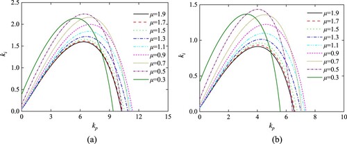
Table 10. Stability region comparison of different μ values for FOPID2D.

Model	μ = 1.9	μ = 1.7	μ = 1.5	μ = 1.3	μ = 1.1	μ = 0.9	μ = 0.7	μ = 0.5	μ = 0.3
G13	10.77	10.96	11.43	12.31	13.59	15.00	15.89	15.70	14.28
G21	4.00	4.11	4.34	4.74	5.34	6.04	6.52	6.45	5.68

Set k_d= 1, k_d2= 1, λ = 0.2 and μ = 0.7, the boundary curves can be drawn and the area sizes stability region can be calculated. Finally, the intersection of stability regions can be determined. It can be observed from Figure 16 and Table 11 that the area of G₂₂ model’s stability region is the smallest. The final area size of FOPID2D controller stability region for the HTGS system is 16.22.

Figure 16. Stability regions of all parameter subsets G₁₁-G₂₄ for FOPID2D.

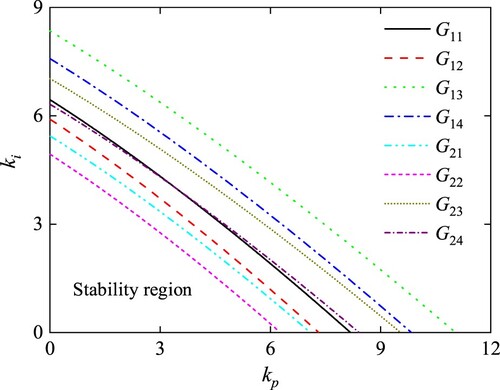
Table 11. Stability region comparison of different parameter subsets for FOPID2D.

Parameter subset	G11	G12	G13	G14	G21	G22	G23	G24
Stability region	27.66	22.65	48.67	39.30	20.21	16.22	35.37	27.91

The following Table 12 lists the result of final stability region area size for the PID, FOPID, PID2D and FOPID2D controllers. Among the four controllers, the area size of FOPID2D controller stability region is largest and the area size of integer PID controller stability region is smallest. It is indicated that the FOPID2D controller has better robust stability than the others.

Table 12. Stability region comparison of PID, FOPID, PID2D and FOPID2D.

Controller	PID	FOPID	PID2D	FOPID2D
Stability region	4.12	13.41	4.69	16.22

5. Conclusion

This paper pays attention to the stability comparison of different controllers for the hydraulic turbine fractional interval parameter time-delay system. First, considering the terms of time-lag and parameter uncertainty and using the advantage of fractional model, the hydraulic turbine fractional order interval parameter time-delay system is obtained with the identification approach and measured data. At the same time, the PID, PID2D, FOPID and FOPID2D controllers are all introduced to the HTGS system. Second, the stability calculation procedure of controller parameter for the hydraulic turbine fractional order interval parameter time-delay system is presented in detail. Third, the variable law of the stable regions of the system with the changing controller parameters is achieved by the analysis of simulation results. At last, the stability region of the four controllers is compared and the results show the advantage of the FOPID2D controller in robust stability and flexibility.

Although the research in this paper is completed by the simulation experiments, these four controllers are applied in the stability comparison of the hydraulic turbine fractional interval parameter time-delay system for the first time. In the future, the research should focus on stability analysis for the nonlinear HTGS system. The nonlinear system model is better than the linear model to describe the dynamic characteristics of the hydraulic turbine governing system. On this basis, the novel research on the control method of the nonlinear HTGS system is the emphasis in the late period.

Disclosure statement

No potential conflict of interest was reported by the author(s).

Data availability

The datasets generated during and/or analysed during the current study are available from the corresponding author upon reasonable request.

Additional information

Funding

This work was supported by the Scientific research planning guidance project of Hubei Provincial Department of Education (grant NO. B2021466).

References

- Chen, Z., Yuan, X., Ji, B., Wang, P., & Tian, H. (2014). Design of a fractional order PID controller for hydraulic turbine regulating system using chaotic non-dominated sorting genetic algorithm II. Energy Conversion and Management, 84, 390–404. https://doi.org/10.1016/j.enconman.2014.04.05
- Hamamci, S. E. (2008). Stabilization using fractional order PI and PID controllers. Nonlinear Dynamics, 51(1), 329–343. https://doi.org/10.1007/s11071-007-9214-5
- Hamamic, S. E. (2007). An algorithm for stabilization of fractional order time delay systems using fractional order PID controllers. IEEE Transactions on Automatic Control, 52(10), 1964–1969. https://doi.org/10.1109/TAC.2008.2007535
- Li, C., & Zhou, J. (2011). Parameters identification of hydraulic turbine governing system using improved gravitational search algorithm. Energy Conversion and Management, 52(1), 374–381. https://doi.org/10.1016/j.enconman.2010.07.012
- Long, Y., Xu, B., Chen, D., & Ye, W. (2018). Dynamic characteristics for a hydro-turbine governing system with viscoelastic materials described by fractional calculus. Applied Mathematical Modelling, 58, 128–139. https://doi.org/10.1016/j.apm.2017.09.052
- Petras, I., Chen, Y. Q., Vinagre, B. M., & Podlubny, I. (2004). Stability of linear time invariant systems with interval fractional orders and interval coefficients. 2004 Second IEEE international conference on computational cybernetics, 30 August 2004–01 September 2004 (pp. 341–346). IEEE. https://doi.org/10.1109/ICCCYB.2004.1437745
- Raju, M., Saikia, L. C., & Sinha, N. (2016). Automatic generation control of a multi-area system using ant lion optimizer algorithm based PID plus second order derivative controller. International Journal of Electrical Power and Energy Systems, 80, 52–63. https://doi.org/10.1016/j.ijepes.2016.01.037
- Sahib, M. A. (2015). A novel optimal PID plus second order derivative controller for AVR system. Engineering Science and Technology, an International Journal, 18(2), 194–206. https://doi.org/10.1016/j.jestch.2014.11.006
- Sain, D., Swain, S. K., Kumar, T., & Mishra, S. K. (2020). Robust 2-DOF FOPID controller design for maglev system using jaya algorithm. IETE Journal of Research, 66(3), 414–426. https://doi.org/10.1080/03772063.2018.1496800
- Tan, N. (2005). Computation of stabilizing PI and PID controllers for processes with time delay. ISA Transactions, 44(2), 213–223. https://doi.org/10.1016/S0019-0578(07)90000-2
- Wei, S. (2011). Simulation of hydraulic turbine regulation system, Huazhong University of science and Technology Press.
- Xian, Y., Xia, C., Zhong, D., & Xu, C. (2019). Chaotic system with coexisting attractors and the stabilization of its fractional order system. Control Theory and Applications, 36(2), 262–270. https://doi.org/10.7641/CTA.2018.70943
- Xu, B., Chen, D., Zhang, H., & Wang, F. (2015). Modeling and stability analysis of a fractional-order francis hydro-turbine governing system. Chaos. Solitons and Fractals, 75, 50–61. https://doi.org/10.1016/j.chaos.2015.01.025
- Xu, B., Chen, D., Zhang, H., Wang, F., Zhang, X., & Wu, Y. (2017). Hamiltonian model and dynamic analyses for a hydro-turbine governing system with fractional item and time-lag. Communications in Nonlinear Science and Numerical Simulation, 47, 35–47. https://doi.org/10.1016/j.cnsns.2016.11.006