Mathematical modeling based on ordinary differential equations: A promising approach to vaccinology

ABSTRACT

New contributions that aim to accelerate the development or to improve the efficacy and safety of vaccines arise from many different areas of research and technology. One of these areas is computational science, which traditionally participates in the initial steps, such as the pre-screening of active substances that have the potential to become a vaccine antigen. In this work, we present another promising way to use computational science in vaccinology: mathematical and computational models of important cell and protein dynamics of the immune system. A system of Ordinary Differential Equations represents different immune system populations, such as B cells and T cells, antigen presenting cells and antibodies. In this way, it is possible to simulate, in silico, the immune response to vaccines under development or under study. Distinct scenarios can be simulated by varying parameters of the mathematical model.

As a proof of concept, we developed a model of the immune response to vaccination against the yellow fever. Our simulations have shown consistent results when compared with experimental data available in the literature. The model is generic enough to represent the action of other diseases or vaccines in the human immune system, such as dengue and Zika virus.

KEYWORDS:

• computational science
• computational modeling
• computational immunology
• computational vaccinology
• immune system
• ordinary differential equations
• yellow fever

Introduction

Computational science is a field that uses computers to study and solve problems from other areas of science and engineering. This broad multidisciplinary field encompasses areas such as computer science, mathematics and physics in order to develop models that can be simulated on computers.

In the same way an architect uses an architectural model to communicate and evaluate his/her ideas, as well as to better study some aspects of an architectural design, a computational scientist can use a computational model to represent and study some aspects of a problem. The model construction starts with the observation and the understanding of the phenomenon that is being investigated. Next, the computational scientist defines the model goals, that is, which questions must be addressed. The model goals define the level of abstraction that must be used. An architectural model can be constructed using distinct scales, depending on the level of details required. Usually the architectural model is constructed at much smaller scale than the original build, and for this reason, details are omitted and only the main aspects of the building are captured. The same occurs with computational models. They also can be constructed using distinct levels of details: the main aspects of the problem are captured by the model and the details, that do not contribute to the solution of the problem, are omitted. If the computational scientist is wrong, and some details are, in fact, key aspects of the model, they can be included in the model later. However, the more detailed the model is, the more challenge is its construction. Indeed, the word model comes from the Latin word modulus that means small measure. So a model represents another entity, usually using less details in its representation.

There are many different ways to model a problem. One way is using mathematics and physics to describe the phenomena associated with the problem. In this case, variables, constants and their relationship are used to characterize the problem that is being studied using a set of equations. Once a model has been defined, a computer simulation can be performed in order to validate the model. Again, there are many ways to execute a simulation on a computer, depending on the form that the model was defined. A useful analogy that can be used to better understand how a simulation is performed on a computer is the process by which an animated movie is made. An animation can be made using a succession of hundreds or thousands of draws, one displayed after the other one with a tiny time interval between them. In a similar way, a simulation can be viewed as the succession of many results. The results are computed using the model's equations. The time can be divided into tiny steps, called time-steps. The computer calculates the values that variables will assume at each time-step, using for this purpose their current values. This process is then repeated until all time-steps were computed. The validation is then performed comparing the results obtained from the simulations with the ones obtained with experiments. The model as well as the constant values can be modified in order to fit the simulation results with the experimental ones.

An interesting aspect about simulations is that, after the model has been validated, the researcher can change the model parameters, as well as the values used as initial conditions for the variables, and observe what happens with the results. Doing so, simulations can help researchers to make predictions about what is the response to different conditions. A larger number of hypotheses can be tested faster than their equivalent experiments, with lower costs and without exposing researchers or participants to risks. Finally, models can be used with optimization purposes. Given a scenario, which variable values can maximize or minimize an output?

Computational science has became so important that the US President's Information Technology Advisory Committee (PITAC) has considered it the third pillar of 21st century science.¹ The report issued by this committee states that “Together with theory and experimentation, computational science now constitutes the ‘third pillar’ of scientific inquiry, enabling researchers to build and test models of complex phenomena.”

A large number of areas make use of computational science: biology, physics, chemistry, engineering, biomechanics, climate modeling, tsunami and earthquake prediction, and so on. Examples of papers that make use of mathematical and computational models can be found in.^2-24

Some simulations try to reproduce or even predict the results obtained from biological experiments. In this case, the expression in silico is used to refer to the experiments that were performed by computers, via a computer simulation. It is an allusion to the in vivo, in vitro and in situ terms, which are commonly used in biology to refer to experiments done in living organisms, outside of living organisms and those that occurs in nature, respectively.

In the vaccinology field, computational science has been used to assist the vaccine development process. In particular, according to DeLisi and Berzofsky²⁵ epitope-mapping algorithms is used for vaccine design since the 1980s. Since then, new computational tools have been used for selection of vaccine targets, see.^26-34 Pappalardo et al.³⁵ present a survey of several computational modeling techniques applied to vaccinology science. Most of the works focus on using computational science to predict epitopes, as the work of Lafuente and Reche,³⁶ or to develop virtual screening approaches, see.^37-40

This work proposes a new use of computational science to vaccinology, in the clinical development stage. With the use of mathematical and computational models, it is possible to experiment, in silico, different scenarios related to vaccination, for answering important questions still open.

Results

As a proof of concept, this section presents the results of a model of the immune response to vaccination against the yellow fever (YF). The model uses a set of equations, that will be described later in the method section, to estimate the concentration of some cells, molecules and virus levels in the body after an individual has been vaccinated against YF. Although YF has been used in this study, it must be stressed that the concept is generic enough to represent the action of other diseases or vaccines in the human immune system.

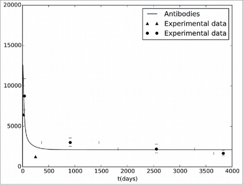
The model can also estimate the concentration of all cells and molecules represented by the equations. For example, Figure 1 shows the antibody dynamics, estimated by the model, after a vaccination against YF. In order to validate the results, we also present, in the same figure, experimental data obtained from the literature. As one can see, the results are consistent with existing literature.

Figure 1. Antibodies curve generated by the computational model. The model simulates the antibody concentrations during a period of 5,000 d. The figure also presents experimental data extracted from Kay et al.⁴¹(▴) and from the collaborative group⁴² (•).

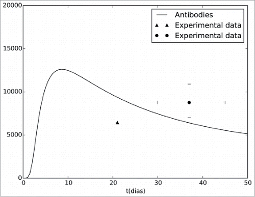
Figure 2 shows the same results presented in Figure 1, but now focusing on the first 50 d after vaccination.

Figure 2. Antibodies curve generated by the computational model. The model simulates the antibody concentrations during a period of 50 d. The figure also presents experimental data extracted from Kay et al.⁴¹(▴) and from the collaborative group⁴² (•).

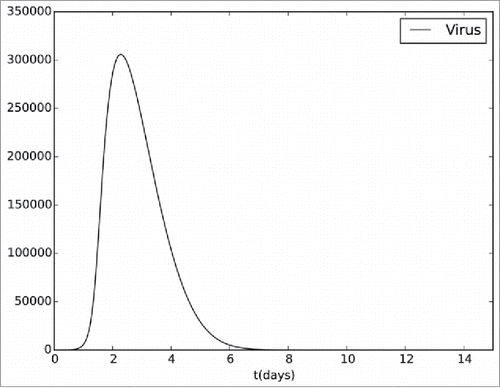
Figure 3 presents the viremia curve produced by the computational model. This curve is qualitatively in accordance with the description found in the YF literature⁴³: the viremia peaks occurs between the second and the third days, and the viral clearance occurs by the seventh day.

Figure 3. Viremia level following the inoculation of the YF vaccine.

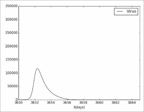
Figure 4 shows the simulation results for the level of viremia after the administration of a booster dose of the YF vaccine. It can be seen that the viremia level now is lower than the one obtained by the first vaccination dose. This is an expected behavior since the immune system respond more rapidly and effectively to a pathogen that has been encountered previously due to the immunological memory. It must be stressed that this result has not been validated.

Figure 4. Viremia level following the booster dose of the YF vaccine 3,650 d (10 years) after the first dose.

Discussion

This section provides discussion about two distinct aspects of the results presented in previous section. The first aspect refers to the numerical results, and the second one refers to the use of computational science in vaccinology.

Computational results

One important aspect about a computational model is its validation. According to Knepell and Arangno,⁴⁴ distinct types of validation can be performed on a computational model. One of the six types of validations is called external validity, which focus on validation as the comparison of simulated and experimental data. An exact match between simulated and experimental data are almost impossible to achieve in biological experiments. The point is to determine whether or not the difference of values between the results are acceptable or not.

As can be seen, the difference of values in Figures 1 and 2 occurs not only between simulated and experimental data, but also in the results of distinct studies, see,^41-42 and among individuals in the same study. This is an implicit characteristic of biological experiments. For this reason, the model tries to adjust its results qualitatively according to the average behavior of the two experimental results used to validate the model. The peak values of antibodies occurs about 10 d after vaccination, then decays and remains almost constant after a long period after vaccination. Some antibody levels predicted by the model fits perfectly to the average experimental levels observed in clinical studies, specially from experiments that used a large number of volunteers, as those obtained by a collaborative group.⁴²

From a qualitative perspective, the model presented in this work predicted accurately the effects of the YF vaccine on the organism (Fig. 3), as well as after the administration of a booster dose of the YF vaccine (Fig. 4). From a quantitative perspective, the model must be better adjusted. Unfortunately, the availability of data in the literature does not allow us to validate the model.

On the use of computational science in vaccinology

The results presented in the previous section show that computational science cannot only be used during the pre-clinical trials, but also, as we argue, in the clinical trials. As stated before, the usage of computational science during this phase of the development of vaccines is not usual. In particular, computational science can help to determine the safe dosage range of a vaccine, prior its administration on volunteers. The idea is quite simple: the effects of multiple dosages can be simulated by a computational model in order to select the best one.

The World Health Organization (WHO) approved a new recommendation that a single dose of YF vaccine provides long-lasting protection. According to WHO,⁴⁵ the 10-year booster dose requirement was removed based on several studies that present evidences that protective antibody levels are found many years after the first vaccination. However, also based on studies, other researchers⁴² claim that more caution should be taken before making a decision like that. Also, computational science can help to decide the need for a booster dose following a primary vaccination, in a similar way we have done in the previous section: simulating, using the actual vaccine dose, the concentration of antibody months, years or decades after the primary dose is given. The anamnestic response can also be simulated in a simple way, computing the values of antibodies after a stimulus of an antigen. Finally, since it can be computed the concentration of all cells, molecules and viruses that compose the model, the active B and T cell activity against the antigen after a certain amount of time that the primary vaccine was administered can be used to predict if a booster dose is necessary or not.

The YF vaccine model used in this work considers the populations of vaccine virus and CD4+ T cells, among others. These populations may have an important role in trying to answer some open issues related to vaccination of YF. One of them is related to the administration of the vaccine in immunocompromised individuals such as those infected by HIV (Human Immunodeficiency Virus), for example. It is observed, in these individuals, a reduction in the population of CD4+ T cells. This reduction directly affects the immune response, and for this reason the administration of vaccines made with live virus, such as the YF vaccine, should be done with caution. With the use of computational models, it is possible to test, in silico, distinct possibilities and scenarios. As the model considers the population of CD4+ T cells, it is possible to reduce their initial amount to simulate the impact of vaccines in HIV infected individual.

These are three examples of situation in which computational science can help in the clinical trials. The use of computational models can help to reduce costs, time, risks and volunteers involved in the process. Of course, to achieve these objectives, models must be reliable. Since models are always an abstraction of reality, using simplifications in order to deal with complexities, many factors that can contribute to the real phenomenon may be ignored during this process.

Material & methods

The mathematical model developed in our previous work to describe the effects of YF in the body was used, in this paper, to reproduce the main stages of the immune response produced by the vaccination against YF. For a review of the mathematical model, see.⁴⁶ Although the mathematical model is the same, some parameters values were modified to represent live attenuated vaccine instead of the active virus.

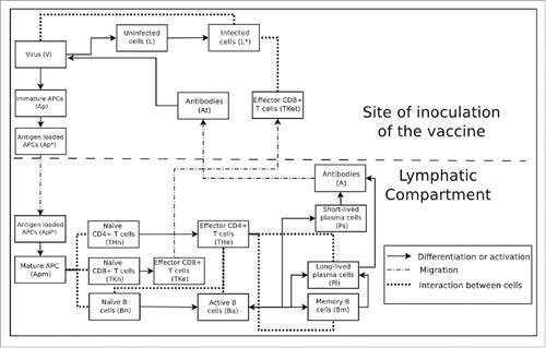
The model considers, in a high level of abstraction, the main populations of cells and molecules involved in this process, which begins when the vaccine viruses are inoculated in the body and, after that, local cells are infected. This infection stimulates immature antigen presenting cells (APCs) present in the site to internalize antigens and become active. These cells then migrate to the lymphoid compartment and become mature, and thus capable of activating naïve cells, such as CD4+ T cells.

The naïve CD4+ T cells, when activated by the action of mature APCs, differentiate into CD4+ T effector cells. They have the function of assisting in the process of recruitment of the population of CD8+ T cells and B cells to help fight infection. The naïve CD8+ T cells, when they are activated with the help of CD4+ T effector cells, differentiate into effector CD8+ T cells which migrate to the site of the vaccine application. The CD8+ T have the function of inducing the apoptosis of infected cells.

The naïve B cells, when active, differentiate into two types of antibody secreting plasma cells, short-lived and long-lived. A portion of active B cells also differentiate into memory B cells, which remain in a rest state until a new exposure to the same virus occurs. When this happens, they become active again, but faster, assisting in the control of infection because they produce antibodies faster. Early produced antibodies will opsonise viruses before they can infect a large number of cells. In addition, memory B cells also maintain long-lived plasma cell levels. Figure 5 shows a simplified scheme that represents populations and interactions represented by the mathematical model using for this purpose Ordinary Differential Equations (ODEs).

Figure 5. Schema of the interaction between all cells, molecules and viruses populations considered in the model.

ODEs is a mathematical tool used to measure the change of a quantity which is determined by another quantity. The change of a quantity is called derivative. In vaccinology, we are interested in the changing of all cells, molecules and viruses concentrations with respect to time.

Each of the ODEs are composed by several terms, as the conventional algebraic equations are. Equation 1, one of the equations that composes our model, is an ODE that represents the virus (V) dynamics.$\frac{dV}{dt}= {\pi }_V\left(V\right)H^{*}- c_{V}V- k_{V}V{A}_t$

π_V (V)H denotes the production of free virions by infected cells (H*), c_V V denotes the non specific virus clearance by the immune system, where c_V is the virus clearance rate. K_vVA_t denotes the specific virus clearance due to the YFV opsonization by antibodies, with a virus clearance rate k_v. A_t represents the population of antibody in the tissue.

This type of equation sometimes has no analytical solution or it may be difficult to solve, so the use of numerical (a.k.a. computational) methods for its resolution is mandatory. The model used in this work consists of 19 ODEs. To solve the ODEs system we implemented a code in Python programming language. Python version 2.7.3 was used. The ODEs was solved using the function odeint.⁴⁷ The experiments were performed on a 2.13 GHz Intel Core i3-M330 processor, with 4 GB RAM. The system runs a 64-bits version of Linux 3.11.10–100.fc18. The complete set of equations and technical aspects of the implementation, as well as the parameters and initial conditions that has not been modified can be found in our previous work.⁴⁶ Table 1 presents the values that has been modified in this work to perform the adjustment to the new experimental data obtained from literature.

Table 1. Values of the modified parameters.

Parameter	Description	Old value	Current value
δBMN	Death rate of memory B cells (day^−1)	0.5	5.0
δS	Death rate of short-lived antibody-secreting plasma cells (day^−1)	0.17	0.5
δL	Death rate of long-lived antibody-secreting plasma cells (day^−1)	1.0 × 10^−2	3.0 × 10^−2
πAS	Secretion rate of antibody titer by unit short-lived plasma cell (day^−1)	1.2	12
πAL	Secretion rate of antibody titer by unit of long-lived plasma cells (day^−1)	0.2	3.0
δA	Clearance rate of antibody (day^−1)	0.15	0.04

Conclusions

The development of vaccines can be divided into two broad stages: a) preclinical development and b) clinical development. Computational science has been used to assist in the pre-clinical development, in particular in the identification of relevant antigens. As a proof of concept, the paper presented the results of a model of the immune response to vaccination against the YF. The model uses a set of ODE to estimate the concentration of some cells, molecules and virus levels in the body after an individual has been vaccinated against YF. From a qualitative point of view, the results obtained by the computational model reproduced the clinical results that can be found in the literature.

Although YF has been used in this study, the concept presented in this work is generic enough to represent the impacts of other vaccines in the human immune system.

As future works, we would like to improve the quantitative results obtained from our model, which will require access to more information that is available in the literature, such as the concentration of CD4+ T cells, CD8 T cells, B cells, an so on.

We believe that in a near future computational science will be used to assist the clinical development of vaccines, in order to a) suggest the optimal dose of a vaccine, b) determine the average vaccination coverage and whether or not a booster dose is necessary, and c) point the differences in the immune response of a vaccine in immunosuppressed individuals.

Abbreviations

APCs	=	antigen presenting cells
CD4	=	cluster of differentiation 4
CD8	=	cluster of differentiation 8
GB	=	Gigabytes
GHz	=	Gigahertz
HIV	=	Human Immunodeficiency Virus
ODE	=	Ordinary Differential Equations
PITAC	=	President's Information Technology Advisory Committee
RAM	=	Random Access Memory
US	=	United States
WHO	=	World Health Organization
YF	=	Yellow fever
YFV	=	Yellow fever virus

Disclosure of potential conflicts of interest

No potential conflicts of interest were disclosed.

Funding

The authors would like to express their thanks to CAPES, CNPq, FAPEMIG and UFJF for funding this work.

References

- US PITA. Committee, Computational Science: Ensuring America's Competitiveness, National Coordination Office for Information Technology Research & Development, URL https://books.google.com.br/books?id=YIhGAAAAYAAJ, 2005
- Schoeberl B, Eichler-Jonsson C, Gilles ED, Müller G. Computational modeling of the dynamics of the MAP kinase cascade activated by surface and internalized EGF receptors. Nat Biotechnol 2002; 20(4):370-375; PMID:11923843; http://dx.doi.org/10.1038/nbt0402-370
- Wiley HS, Shvartsman AY, Lauffenburger DA. Computational modeling of the EGF-receptor system: a paradigm for systems biology, TICB 2003; 13(1):43-50; PMID:12480339
- Doddi SK, Bagchi P. Three-dimensional computational modeling of multiple deformable cells flowing in microvessels. Physical Review E 2009; 79(4):046318; http://dx.doi.org/10.1103/PhysRevE.79.046318
- Beard DA, Schlick T. Computational modeling predicts the structure and dynamics of chromatin fiber. Structure 2001; 9(2):105-114; PMID:11250195; http://dx.doi.org/10.1016/S0969-2126(01)00572-X
- Querec TD, Akondy RS, Lee EK, Cao W, Nakaya HI, Teuwen D, Pirani A, Gernert K, Deng J, Marzolf B, et al. Systems biology approach predicts immunogenicity of the yellow fever vaccine in humans. Nat Immunol 2009; 10 (1):116-125; PMID:19029902; http://dx.doi.org/10.1038/ni.1688
- Karr JR, Sanghvi JC, Macklin DN, Gutschow MV, Jacobs JM, Bolival B, Assad-Garcia N, Glass JI, Covert MW. A whole-cell computational model predicts phenotype from genotype. Cell 2012; 150(2):389-401; PMID:22817898; http://dx.doi.org/10.1016/j.cell.2012.05.044
- Clarke S, Vvedensky DD. Origin of reflection high-energy electrondiffraction intensity oscillations during molecular-beam epitaxy: A computational modeling approach. Phys Rev Lett 1987; 58(21):2235; PMID:10034688; http://dx.doi.org/10.1103/PhysRevLett.58.2235
- Sakurai T. Computational modeling of magnetic fields in solar active regions. Space Sci Rev 1989; 51(1-2):11-48
- Cuitino AM, Ortiz M. Computational modelling of single crystals. Modelling Simulation Materials Sci Engineering 1993; 1(3):225; http://dx.doi.org/10.1088/0965-0393/1/3/001
- Yanez J, Kuznetsov M. An analysis of flame instabilities for hydrogen-air mixtures based on Sivashinsky equation. Phys Lett A 2016; 380(33):2549-2560; http://dx.doi.org/10.1016/j.physleta.2016.05.048
- Feldgus S, Landis CR. Large-scale computational modeling of Rh (DuPHOS)]+-catalyzed hydrogenation of prochiral enamides: reaction pathways and the origin of enantioselection. J Am Chem Soc 2000; 122(51):12714-12727; http://dx.doi.org/10.1021/ja0019373
- Bicerano J. Computational modeling of polymers. Plastics Engineering (Book 25). Taylor & Francis, 1992
- Rots JG. Computational modeling of concrete fracture. Ph.D. thesis. Technische Hogeschool Delft, 1988
- Schafer B, Peköz T. Computational modeling of cold-formed steel: characterizing geometric imperfections and residual stresses. J Constructional Steel Res 1998; 47(3):193-210; http://dx.doi.org/10.1016/S0143-974X(98)00007-8
- Roussel N, Geiker MR, Dufour F, Thrane LN, Szabo P. Computational modeling of concrete flow: general overview. Cement Concrete Res 2007; 37(9):1298-1307; http://dx.doi.org/10.1016/j.cemconres.2007.06.007
- McHugh P, Asaro R, Shih C. Computational modeling of metal matrix composite materials-I. Isothermal deformation patterns in ideal microstructures. Acta Metallurgica Et Materialia 1993; 41(5):1461-1476; http://dx.doi.org/10.1016/0956-7151(93)90255-Q
- Porter B, Zauel R, Stockman H, Guldberg R, Fyhrie D. 3-D computational modeling of media flow through scaffolds in a perfusion bioreactor. J Biomech 2005; 38(3):543-549; PMID:15652553; http://dx.doi.org/10.1016/j.jbiomech.2004.04.011
- Kuhl E, Maas R, Himpel G, Menzel A. Computational modeling of arterial wall growth. Biomech Model Mechanobiol 2007; 6(5):321-331; PMID:17119902; http://dx.doi.org/10.1007/s10237-006-0062-x
- Randall DA, Ringler TD, Heikes RP, Jones P, Baumgardner J. Climate modeling with spherical geodesic grids. Comput Sci Eng 2002; 4(5):32-41; http://dx.doi.org/10.1109/MCISE.2002.1032427
- Nefedova V, Jacob R, Foster I, Liu Z, Liu Y, Deelman E, Mehta G, Su MH, Vahi K. Automating climate science: Large ensemble simulations on the TeraGrid with the GriPhyN Virtual Data System. In: 2006 Second IEEE International Conference on e-Science and Grid Computing (e-Science’06), IEEE, 32-32, 2006
- Bernholdt D, Bharathi S, Brown D, Chanchio K, Chen M, Chervenak A, Cinquini L, Drach B, Foster I, Fox P, et al. The Earth System Grid: Supporting the Next Generation of Climate Modeling Research. Proc IEEE Inst Electr Electron Eng 2005; 93(3):485-495; http://dx.doi.org/10.1109/JPROC.2004.842745
- Das S, Aki K. Fault plane with barriers: a versatile earthquake model. J Geophys Res 1977; 82(36):5658-5670; http://dx.doi.org/10.1029/JB082i036p05658
- Loomis HG. Tsunami prediction using the reciprocal property of Green's functions. Marine Geodesy 1979; 2(1):27-39; http://dx.doi.org/10.1080/15210607909379333
- DeLisi C, Berzofsky JA. T-cell antigenic sites tend to be amphipathic structures. Proc Natl Acad Sci 1985; 82(20):7048-7052; PMID:2413457; http://dx.doi.org/10.1073/pnas.82.20.7048
- Kumar N, Hendriks BS, Janes KA, Graaf D, Lauffenburger DA. Applying computational modeling to drug discovery and development. Drug Discov Today 2006; 11(17–18):806-811; PMID:16935748; http://dx.doi.org/10.1016/j.drudis.2006.07.010
- Groot AS, Moise L, McMurry JA, Martin W. Epitope-Based Immunome-Derived Vaccines: A Strategy for Improved Design and Safety. In: Falus A, ed. Clinical Applications of Immunomics. New York: Springer, 2009:39-69
- Oliveira FM, Coelho IE, Lopes MD, Taranto AG, Junior MC, Santos LL, Villar JA, Fonseca CT, Lopes DD. The Use of Reverse Vaccinology and Molecular Modeling Associated with Cell Proliferation Stimulation Approach to Select Promiscuous Epitopes from Schistosoma mansoni. Appl Biochem Biotechnol 2016; 179(6):1023-1040; PMID:26979443; http://dx.doi.org/10.1007/s12010-016-2048-1
- Rappuoli R, Bottomley MJ, D'Oro U, Finco O, Gregorio E. Reverse vaccinology 2.0: Human immunology instructs vaccine antigen design. J Exp Med 2016; 213(4):469-481; PMID:27022144; http://dx.doi.org/10.1084/jem.20151960
- Michalik M, Djahanshiri B, Leo JC, Linke D. Reverse Vaccinology: The Pathway from Genomes and Epitope Predictions to Tailored Recombinant Vaccines. Methods Mol Biol 2016; 1403:87-106; PMID:27076126; http://dx.doi.org/10.1007/978-1-4939-3387-7_4
- Andreoni F, Amagliani G, Magnani M. Selection of Vaccine Candidates for Fish Pasteurellosis Using Reverse Vaccinology and an In Vitro Screening Approach. Methods Mol Biol 2016; 1404:181-192; PMID:27076298; http://dx.doi.org/10.1007/978-1-4939-3389-1_12
- Yang YT, Chow YH, Hsiao KN, Hu KC, Chiang JR, Wu SC, Chong P, Liu CC. Development of a full-length cDNA-derived enterovirus A71 vaccine candidate using reverse genetics technology. Antiviral Res 2016; 132:225-232; PMID:27387826; http://dx.doi.org/10.1016/j.antiviral.2016.06.014
- Meunier M, Guyard-Nicodème M, Hirchaud E, Parra A, Chemaly M, Dory D, Identification of Novel Vaccine Candidates against Campylobacter through Reverse Vaccinology. J Immunol Res 2016:5715790; PMID:27413761; http://dx.doi.org/10.1155/2016/5715790
- Groot AS, Bosma A, Chinai N, Frost J, Jesdale BM, Gonzalez MA, Martin W, Saint-Aubin C. From genome to vaccine: in silico predictions, ex vivo verification. Vaccine 2001; 19(31):4385-4395; PMID:11483263; http://dx.doi.org/10.1016/S0264-410X(01)00145-1
- Pappalardo F, Flower D, Russo G, Pennisi M, Motta S. Computational modelling approaches to vaccinology. Pharmacol Res 2015; 92:40-45; PMID:25224605; http://dx.doi.org/10.1016/j.phrs.2014.08.006
- Lafuente EM, Reche PA. Prediction of MHC-peptide binding: a systematic and comprehensive overview. Curr Pharm Des 2009: 15(28):3209-3220; PMID:19860671; http://dx.doi.org/10.2174/138161209789105162
- Gomez-Bombarelli R, Aguilera-Iparraguirre J, Hirzel TD, Duvenaud D, Maclaurin D, Blood-Forsythe MA, Chae HS, Einzinger M, Ha DG, Wu T, et al. Design of efficient molecular organic light-emitting diodes by a highthroughput virtual screening and experimental approach. Nat Mater 2016; 15(10):1120-7; advance online publication; PMID:27500805; http://dx.doi.org/10.1038/nmat4717
- Geanes AR, Cho HP, Nance KD, McGowan KM, Conn PJ, Jones CK, Meiler J, Lindsley CW. Ligand-based virtual screen for the discovery of novel M5 inhibitor chemotypes. Bioorg Med Chem Lett 2016; 26(18):4487-4491; PMID:27503678; http://dx.doi.org/10.1016/j.bmcl.2016.07.071
- Xu Y, Yue L, Wang Y, Xing J, Chen Z, Shi Z, Liu R, Liu YC, Luo X, Jiang H, et al. Discovery of Novel Inhibitors Targeting Menin-Mixed Lineage Leukemia (MLL) Interface Using Pharmacophore- and Docking-Based Virtual Screening. J Chem Inf Model 2016; 56(9):1847-55; ; PMID:27513308; http://dx.doi.org/10.1021/acs.jcim.6b00185
- Khalili S, Mohammadpour H, Shokrollahi Barough M, Kokhaei P. ILP-2 modeling and virtual screening of an FDA-approved library:a possible anticancer therapy. Turk J Med Sci 2016; 46(4):1135-1143; PMID:27513416; http://dx.doi.org/10.3906/sag-1503-2
- Kay A, Chen LH, Sisti M, Monath TP. Yellow fever vaccine seroconversion in travelers. Am J Trop Med Hyg 2011; 85(4):748-749; PMID:21976582; http://dx.doi.org/10.4269/ajtmh.2011.11-0363
- Collaborative group. Duration of post-vaccination immunity against yellow fever in adults. Vaccine 2014; 32(39):4977-4984; PMID:25090646; http://dx.doi.org/10.1016/j.vaccine.2014.07.021
- Monath TP, Gershman M, Staples EJ, Barrett ADT. Yellow fever vaccine. In: Plotkin SA, Orenstein WA, Offit PA, eds. Vaccines. 6th ed. Saunders Elsevier, 2012:870-896
- Knepell PL, Arangno DC. Simulation Validation: A Confidence Assessment Methodology. Wiley, 1993
- WHO. Vaccines and vaccination against yellow fever. Wkly Epidemiol Rec 2013; 88(27):269-283; PMID:23909008
- Bonin C, Santos RW, Fernandes GC, Lobosco M. Computational modeling of the immune response to yellow fever. J Comp Appl Math 2016; 295:127-138; http://dx.doi.org/10.1016/j.cam.2015.01.020
- Odeint, Odeint's Homepage, URL http://docs.scipy.org, 2014