Determining the hydraulic properties of coastal aquifer systems using groundwater response to tidal fluctuations: applicability and limitations

ABSTRACT

Determination of the hydraulic properties of a coastal aquifer system with lower cost and acceptable accuracy has practical implications. Although many theoretical solutions have been developed over recent decades, most of them assume that an aquifer system extends inland and subjected a single-frequency tidal fluctuation on coastline boundary. In addition, only one hydraulic parameter, i.e., the hydraulic diffusivity, of an aquifer can be obtained in most cases. In this paper, the solution of groundwater response in a leaky confined coastal aquifer to dual frequency tidal fluctuations has been established. The new solution was then used as an example to discuss the applicability and limitations of using tidal fluctuations for determining coastal aquifer hydraulic properties. Our study illustrated that ocean tides could only transport to a limited distance towards inland depending on the coastal aquifer hydraulic properties. The tidal method is applicable only when changes in the hydraulic head within in a monitoring well can be detected with an acceptable accuracy. Both the hydraulic diffusivity and leakage can be identified from the monitored hydraulic heads. By incorporating the use of aquifer thickness, the transmissivity and storage coefficient of a perfectly confined aquifer can also be simultaneously estimated.

KEYWORDS:

• Leaky confined costal aquifer
• dual-frequency ocean tides
• analytical solution
• tidal effects
• characterization of hydrogeological properties
• limitations of traditional methods

1. Introduction

Characterization of the hydraulic properties of coastal aquifer systems has important implications that cover a number of research topics, such as geotechnical engineering (Farrell 1994), assessment of water resources (Jha et al. 2008; Befus et al. 2017; Singaraja, Chidambaram, and Jacob 2018), submarine groundwater discharge (Moore 1996; Taniguchi 2002; Prieto and Destouni 2011), seawater intrusion (Carr 1969; Kuan et al. 2012), and migration of contaminants, nutrients, and land-sourced solute (Chan and Mohsen 1992; Gallagher et al. 1996; Uchiyama et al. 2000; Liu, Jiao, and Luo 2016). Although several direct hydraulic testing methods, such as the use of permeameters or seepage meters, slug test, tracer test, pumping test, and a few indirect methods, such as grain-size analysis (Michael et al. 2003; Millham and Howes 1995), are available, the tidal method is simple and inexpensive, and can obtain compatible results with the pumping test (Carr and Van Der Kamp 1969). In addition, the hydraulic properties obtained by the tidal method can also be considered more representative to large-scale hydrogeological characteristics because the results are derived from the signals of hydraulic heads transmitted from the coastline where ocean tides are imposed across a long distance to the monitoring well at which fluctuations of hydraulic head are detected.

The studies on tide-induced groundwater flow can be traced back to the 1950 s. Jacob (1950) developed the solution that considers one-dimensional flow within a confined, semi-infinite coastal aquifer in the direction orthogonal to the straight coastline. Over recent decades, analytical solutions that consider different types of coastal aquifer system, or models have been developed, as briefly reviewed below.

The simplest model consists of a single, semi-infinite, unconfined aquifer with vertical beach and straight coastline (Ferris 1952; Yeh et al. 2010). To consider the combined effects of tidal loading from an estuary, Sun (1997) derived a two-dimensional analytical solution for a confined nonleaky aquifer (popularly called L-shaped coastal aquifer). A more generalized analytical solution was developed by Li et al. (2000) in which the interaction between cross-and along-shore tidal waves in the aquifer area near the estuary’s entry has been taken into account. To consider three water-land boundaries (i.e. two estuaries, and popularly called U-shaped coastal aquifer), Huang et al. (2015) derived the analytical solution. The analytical solution that considers inclined angles of beach slope and impervious ocean bed together with rainfall has also been developed by Hsieh et al. (2015). In addition, analytical solutions for an unconfined aquifer with two hydraulically different zones across inland direction (Guo, Jiao, and Li 2010), a confined aquifer sandwiched in between impermeable roof and bottom with consideration of linear increase in hydraulic conductivity toward the inland (Bonachesi and Guarracino 2011), and an unconfined aquifer with a finite width and sediment cover at two sides (Rotzoll, EI-Dadi, and Gingerich 2008) are also available.

The sophisticated, analytical solutions that consider multiple layers in coastal aquifer systems have been developed by many researchers. Representative models include, but not limited to, those that consist of a confined aquifer overlapped by a semipermeable layer with a finite width (two-layer model) and subjected to tidal fluctuations at both sides (Sun et al. 2008), a semi-infinite, unconfined top aquifer and a leaky bottom aquifer with a semipermeable layer sandwiched between them (three-layer model) (Jiao and Tang 1999; Li and Jiao 2002a; Wang et al. 2018), three-layer model with an L-shaped boundary (Li and Jiao 2002b), three-layer model with a finite width and tidal loading at two sides to simulate a narrow island (Huang, Yeh, and Chang 2012), three-layer model with the lower two layers partially extended under the sea (Li and Jiao 2001), and three-layer model but having different hydraulic properties in a finite zone close to the sea (Asadi-Aghbolaghi, Chuang, and Yeh 2014). A more generalized theoretical solution for the three-layer model has recently been developed by Zhao et al. (2019) in which the aquifer length is assumed to be finite and the solution for the semi-infinite three-layer aquifer can be considered as a special case of the generalized solution.

In almost all of the above theoretical studies, a single-frequency, either sinusoidal or cosinusoidal, tidal fluctuations are assumed as boundary conditions for the coastline and estuary with an exception by Guo, Jiao, and Li (2010). Although the shape of sinusoidal waves is similar to that of cosinusoidal waves, physically, tidal fluctuations should be expressed in terms of cosinusoidal functions (Butikow 2000). In addition, tidal fluctuations consist of multiple constituents in reality, and several constituents can be simultaneously detected in practice, such as lunar diurnal (O₁) and lunisolar diurnal (K₁) (Trefry and Bekele 2004), O₁ and principal lunar semidiurnal (M₂) (Koizumi 1998; Rotzoll, EI-Dadi, and Gingerich 2008). Furthermore, the magnitude of hydraulic head induced by the ocean tides decays in a coastal aquifer with increase in the distance from coastline, and eventually becomes undetectable at a certain distance (e.g. 5 km) reported by Rotzoll and EI-Kadi (2008), but most researchers applied the tidal method without providing an obvious evidence that the changes in hydraulic head in a monitoring well were in deed directly induced by the ocean tides, especially when a monitoring well is more than several kilometers far away from the coastline. Be aware that similar changes in hydraulic head in an inland well can also be detected due to Earth tides with similar frequencies of ocean tides (Liao and Wang 2018).

To address the above problems, and to discuss the applicability and limitations of using the tidal method for determining the hydraulic properties of coastal aquifer systems, we derive an analytical solution for a semi-infinite, three-layer aquifer system with dual-frequency tidal fluctuations, as an example for simulating multiple-frequency tidal fluctuations which are closer to reality. We then use the new solution to demonstrate the possibility of identifying the hydraulic properties from “synthetically” monitored data with noises based on the method of least squares. We also discuss the possible distance at which changes in hydraulic head in a monitoring well that can be detected with an acceptable accuracy for providing referential information about how to select an appropriate location for setting a monitoring well in practice. Furthermore, we propose an approach for estimating both the transmissivity and storage coefficient based on measurement data to facilitate wider use of the technology in coastal engineering.

2. Mathematical model and analytical solution

2.1. Mathematical model

The schematic diagram illustrating a semi-infinite, three-layer coastal aquifer system imposed by dual-frequency tidal fluctuations on the coastline is depicted in Figure 1. The three-layer aquifer system consists of a leaky confined aquifer on an impermeable ocean-bed, overlapped with a semi-impermeable aquitard, and then an unconfined aquifer on the top. Groundwater level in the top unconfined aquifer is assumed to be the same as mean sea level and constant for simplicity.

Figure 1. Schematic diagram of a semi-infinite, leaky confined coastal aquifer system imposed by dual-frequency ocean tides on the coastline boundary (modified from Li and Jiao 2002a)

One-dimensional transient flow of groundwater through the leaky confined aquifer can be expressed by the following equation (e.g. Jiao and Tang 1999):

(1) $S\frac{\mathrm{\partial }h}{\mathrm{\partial }t}=T\frac{{\mathrm{\partial }}^{2}h}{\mathrm{\partial }{x}^2}+L\left(h_z-h\right)$(1)

where h, specifically h(x, t), is the hydraulic head [L], T is the transmissivity [L² T⁻¹], S is the storage coefficient (dimensionless), h_z is the constant, groundwater level [L] in the top unconfined aquifer, L is the specific leakage [T⁻¹] of semi-impermeable aquitard, t is the time [T], and x is the distance from coastline [L].

The boundary condition on coastline, i.e. x = 0, is

(2) $h(0,t)=h_z+\sum _{i=1}^2{A}_{i}cos\left({\omega }_{i}t+c_i\right)$(2)

in which, A_i, ω_i, and c_i are the amplitude, speed, and phase shift of the ith tidal constituent, respectively. Here, we use i = 1 to 2 to simulate dual-frequency tidal fluctuations. The boundary condition on the inland side can be assumed to be a constant head as expressed in Equation (3(3) $h\left(\mathrm{\infty },t\right)=h_z$(3) ), or no-flow, without influence on theoretical solution, because the tidal fluctuations have no effect far inland as x approaches infinity.

(3) $h\left(\mathrm{\infty },t\right)=h_z$(3)

2.2. Analytical solution

The solution to the Equation (1(1) $S\frac{\mathrm{\partial }h}{\mathrm{\partial }t}=T\frac{{\mathrm{\partial }}^{2}h}{\mathrm{\partial }{x}^2}+L\left(h_z-h\right)$(1) ), together with the boundary conditions can be obtained as follows, with a similar approach adopted by Sun (1997) and Jiao and Tang (1999) for solving the single-frequency tidal fluctuation problems.

(4) $h\left(x,t\right)=h_z+\sum _{i=1}^2{A}_i{e}^{-{\delta }_{i}x}cos\left({\omega }_{i}t-\frac{{\omega }_{i}S}{2{\delta }_{i}T}x+c_i\right)$(4)

in which,

(5) ${\delta }_i=\frac{1}{\sqrt{2}}{\left\{{\left[{\left(\frac{L}{T}\right)}^2+{\left(\frac{{\omega }_{i}S}{T}\right)}^2\right]}^{1/2}+\frac{L}{T}\right\}}^{1/2},i=1,2$(5)

Let D = T/S, and M = L/T, the Equations (4)(4) $h\left(x,t\right)=h_z+\sum _{i=1}^2{A}_i{e}^{-{\delta }_{i}x}cos\left({\omega }_{i}t-\frac{{\omega }_{i}S}{2{\delta }_{i}T}x+c_i\right)$(4) and (5(5) ${\delta }_i=\frac{1}{\sqrt{2}}{\left\{{\left[{\left(\frac{L}{T}\right)}^2+{\left(\frac{{\omega }_{i}S}{T}\right)}^2\right]}^{1/2}+\frac{L}{T}\right\}}^{1/2},i=1,2$(5) ) can then be rewritten as follows:

(6) $h\left(x,t\right)=h_z+\sum _{i=1}^2{A}_i{e}^{-{\delta }_{i}x}cos\left({\omega }_{i}t-\frac{{\omega }_i}{2{\delta }_{i}D}x+c_i\right)$(6)

(7) ${\delta }_i=\frac{1}{\sqrt{2}}{\left\{{\left[M^2+{\left(\frac{{\omega }_i}{D}\right)}^2\right]}^{1/2}+M\right\}}^{1/2},i=1,2$(7)

where D is the hydraulic diffusivity [L² T⁻¹], a well-known and commonly used hydrogeological parameter. M is the ratio of specific leakage of semi-impermeable aquitard to the transmissivity of leaky confined aquifer [L⁻²].

3. Analytical simulations

3.1. Time-dependent variations of hydraulic head within the leaky confined aquifer

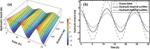
The transmissivity is the product of aquifer thickness and hydraulic conductivity (Hantush 1964), which mainly depends on aquifer porosity and the connectivity between pores. The storage coefficient is the product of aquifer thickness and specific storage (Hantush 1964), which depends on several factors including the interconnected porosity, bulk compressibility, matrix compressibility, and the compressibility of pore fluid itself. The values of both parameters may range over several orders of magnitude even for the same type of geological formation (Nelson 1994; Zhang et al. 2000). Similarly, the leakage of an aquitard may also vary widely. In addition, ocean tides are formed by the gravitational attraction of the Moon and Sun on the water in the ocean and behave differently in different places in the world. Therefore, it is difficult to determine the so-called representative values for related parameters. For the analytical simulations, we assumed that the ocean tides were composed of M₂ and lunar elliptical semidiurnal (N₂) constituents. Correspondingly, ω₁ and ω₂ are equivalent to 0.506 h⁻¹ and 0.496 h⁻¹, respectively. In addition, we assumed that the amplitude and phase shift for M₂ and N₂ to be 2.687 m and 0.543 m, and 0.7012 and 0; and the hydraulic diffusivity, D, and the ratio of leakage to the transmissivity, M, to be 2 × 10⁶ m²/day and 2.5 × 10⁵/m², respectively. The mean sea level and groundwater level in the top unconfined aquifer was set to be 0 m for simplicity. With these assumptions, the time-dependent variations of the hydraulic head within the leaky confined aquifer extends inland, and at the distances of x = 100 m and 200 m can be simulated as an example, and illustrated in Figure 2(a-b), respectively.

Figure 2. The response of hydraulic head within the leaky confined aquifer due to dual-frequency tidal fluctuations: (a) time-dependent variations over x = 0 to 300 m; (b) time-dependent variations at x = 100 m and 200 m, and compared with ocean tides

3.2. Effects of hydraulic diffusivity and leakage

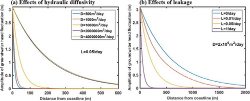
The effects of the hydraulic diffusivity and leakage on the transport of ocean tides within the leaky confined aquifer can be simulated by changing the value of one parameter over a certain range while keeping other parameters being fixed. The changes in decay of ocean tidal amplitude, equivalent to the maximum hydraulic head within the leaky confined aquifer, across the distance from coastline due to the changes in hydraulic diffusivity and leakage are depicted in Figure 3(a–b), respectively.

Figure 3. The effects of aquifer system hydraulic properties on the transport of ocean tides within the leaky confined aquifer: (a) effects of the hydraulic diffusivity of leaky confined aquifer; (b) effects of the leakage of semi-impermeable aquitard

Although the use of high sensitivity sensors can make it possible to detect the fluctuations of hydraulic head at millimeter or even sub-millimeter levels, the recorded results may contain noises and signals induced by other factors, such as changes in temperature and local atmospheric pressure. As an example, we assume reliable measurement for the hydraulic head in this theoretical discussion is greater than 0.1 of the maximum amplitude of ocean tides. Table 1 shows the maximum distances at which the requirement is met under different combinations of hydraulic diffusivity and leakage. Assignment of reliable measurements to other levels can also be performed with a similar approach corresponding to the required accuracy and the sensitivity of sensors.

Table 1. The distance(m) at which the hydraulic head within the confined aquifer decays to 0.1 of the maximum amplitude of ocean tides

	D (Hydraulic diffusivity)(m^2/day)
L (Leakage) (day)^−1	500	1000	10,000	2,000,000	40,000,000
0	20.9637	29.6455	93.7434	1325.81	5929.25
0.05	20.952	29.6146	92.7829	457.219	471.344
1	20.7486	29.0907	76.7228	102.978	104.496

3.3. Identification of hydraulic parameters

To theoretically examine the accuracy for identifying the hydraulic parameters, specifically, the hydraulic diffusivity, D, and the ratio of leakage to the transmissivity, M, we synthetically produce two sets of monitored data at x = 200 m, as an example, with different noises by using the Equations (6)(6) $h\left(x,t\right)=h_z+\sum _{i=1}^2{A}_i{e}^{-{\delta }_{i}x}cos\left({\omega }_{i}t-\frac{{\omega }_i}{2{\delta }_{i}D}x+c_i\right)$(6) and (7(7) ${\delta }_i=\frac{1}{\sqrt{2}}{\left\{{\left[M^2+{\left(\frac{{\omega }_i}{D}\right)}^2\right]}^{1/2}+M\right\}}^{1/2},i=1,2$(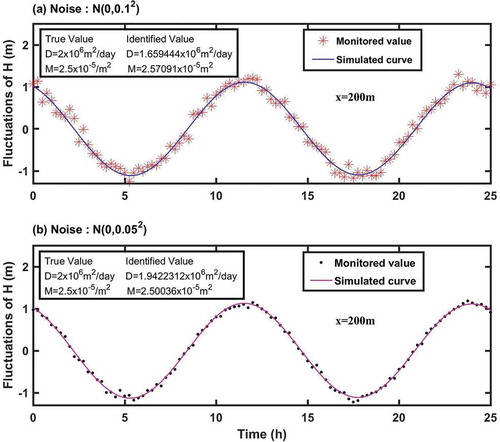7) ) together with the same values for individual parameters as assumed in 3.1, and Gauss white noises: N(0, 0.1²) and N(0, 0.05²). The time interval was set to be 0.25 hour, and the time period for the measurement was set to be 25 hours (totally, 101 synthetically produced measurement data). Hereafter, we call the values of D and L input for the simulation as “true values,” and synthetically produced measurement data as “monitored hydraulic head.”

Identification of the hydraulic parameters can be performed by the method of least squares for minimizing the following error function:

(8) $\begin{array}{rl}& \sum _{i=1}^{101}\left[\left(x=200m,t_i,D,M\right)\right.\\ & -h_m\left(x=200m,t_i,D=2\times {10}^6{m}^2/\right.day,\\ & M=2.5\times {10}^{-5}/{\left.\left.m^2\right)\right]}^2\end{array}$(8)

in which h_c is the calculated hydraulic head with D and M as unknown parameters, and h_m is the monitored hydraulic head at x = 200 m. The identified values for D and M together with the monitored hydraulic heads and simulated curves using identified values and the Equations (6)(6) $h\left(x,t\right)=h_z+\sum _{i=1}^2{A}_i{e}^{-{\delta }_{i}x}cos\left({\omega }_{i}t-\frac{{\omega }_i}{2{\delta }_{i}D}x+c_i\right)$(6) and (7(7) ${\delta }_i=\frac{1}{\sqrt{2}}{\left\{{\left[M^2+{\left(\frac{{\omega }_i}{D}\right)}^2\right]}^{1/2}+M\right\}}^{1/2},i=1,2$(7) ) are illustrated in Figure 4a for the noise: N(0, 0.1²), and (b) for the noise: N(0, 0.05²), respectively. When the noise was at N(0, 0.1²), the identified values for the hydraulic diffusivity, D, and the ration of leakage to transmissivity, M, were 1.659444 × 10⁶ m²/day, and 2.57091 × 10⁻⁵/m², corresponding to relative errors of 17.03% and 2.84%, respectively. When the noise was at N(0, 0.05²), the identified values for D and M, were 1.9422312 × 10⁶ m²/day, and 2.50036 × 10⁻⁵/m², corresponding to relative errors of 2.89% and 0.01%, respectively.

Figure 4. Comparisons between identified hydraulic parameters and true values, and simulated curves and monitored hydraulic heads: (a) noise = N(0, 0.1²); (b) noise = N(0, 0.05²)

4. Discussion

4.1. Comparison with existing analytical solutions

Equation (6)(6) $h\left(x,t\right)=h_z+\sum _{i=1}^2{A}_i{e}^{-{\delta }_{i}x}cos\left({\omega }_{i}t-\frac{{\omega }_i}{2{\delta }_{i}D}x+c_i\right)$(6) expresses the superposition of hydraulic heads induced by two tides with different frequencies. If only a single-frequency ocean tide is imposed on the coastline boundary, Equation (6)(6) $h\left(x,t\right)=h_z+\sum _{i=1}^2{A}_i{e}^{-{\delta }_{i}x}cos\left({\omega }_{i}t-\frac{{\omega }_i}{2{\delta }_{i}D}x+c_i\right)$(6) can be reduced as:

(9) $h\left(x,t\right)=h_z+A{e}^{-\delta x}cos\left(\omega t-\delta x+c\right)$(9)

in which, δ is the same as defined in Equation (7)(7) ${\delta }_i=\frac{1}{\sqrt{2}}{\left\{{\left[M^2+{\left(\frac{{\omega }_i}{D}\right)}^2\right]}^{1/2}+M\right\}}^{1/2},i=1,2$(7) .

Equations (9)(9) $h\left(x,t\right)=h_z+A{e}^{-\delta x}cos\left(\omega t-\delta x+c\right)$(9) and (7(7) ${\delta }_i=\frac{1}{\sqrt{2}}{\left\{{\left[M^2+{\left(\frac{{\omega }_i}{D}\right)}^2\right]}^{1/2}+M\right\}}^{1/2},i=1,2$(7) ) are the same as the solution derived by Jiao and Tang (1999) for the same three-layer hydrogeological model but imposed by single-frequency ocean tides, although different symbols are used for a few parameters. If there is no leakage, i.e. L = 0, the solution can be further reduced to the following Equation (10)(10) $h\left(x,t\right)=h_z+A{e}^{-\sqrt{\frac{\omega S}{2T}}x}cos\left(\omega t-\sqrt{\frac{\omega S}{2T}}x+c\right)$(10) which is essentially the same as the solution derived by Ferris (1951) for a perfectly confined coastal aquifer.

(10) $h\left(x,t\right)=h_z+A{e}^{-\sqrt{\frac{\omega S}{2T}}x}cos\left(\omega t-\sqrt{\frac{\omega S}{2T}}x+c\right)$(10)

Therefore, the newly derived Equation (6)(6) $h\left(x,t\right)=h_z+\sum _{i=1}^2{A}_i{e}^{-{\delta }_{i}x}cos\left({\omega }_{i}t-\frac{{\omega }_i}{2{\delta }_{i}D}x+c_i\right)$(6) together with Equation (7)(7) ${\delta }_i=\frac{1}{\sqrt{2}}{\left\{{\left[M^2+{\left(\frac{{\omega }_i}{D}\right)}^2\right]}^{1/2}+M\right\}}^{1/2},i=1,2$(7) can be considered as a generalized theoretical solution for the three-layer coastal aquifer system imposed by multiple tidal constituents. If the numbers of tidal constituents are more than two, the solution can also be obtained by increasing the number of i in the Equation (6)(6) $h\left(x,t\right)=h_z+\sum _{i=1}^2{A}_i{e}^{-{\delta }_{i}x}cos\left({\omega }_{i}t-\frac{{\omega }_i}{2{\delta }_{i}D}x+c_i\right)$(6) and performing superposition.

4.2. Characteristics of time-dependent hydraulic heads within the leaky confined aquifer

Apparently, the wave shape looks like a single-frequency tide (Figure 2), this is because the frequencies of the two tidal constituents, i.e. M₂ and N₂, considered in this theoretical study are close to each other. The amplitude of ocean tides, corresponding to the manganite of hydraulic head within the leaky confined aquifer decays exponentially accompanying a time-lag with increase in distance, x, toward inland (Equation (6(6) $h\left(x,t\right)=h_z+\sum _{i=1}^2{A}_i{e}^{-{\delta }_{i}x}cos\left({\omega }_{i}t-\frac{{\omega }_i}{2{\delta }_{i}D}x+c_i\right)$(6) ), and Figure 2(a–b)). The hydraulic head will eventually decay to the level at which it cannot be detected with a reliable accuracy or below the resolution of a hydraulic sensor. Tidal method is applicable only within the distance at which the decayed hydraulic head can be reliably detected.

4.3. Effects of hydraulic diffusivity and leakage

Both the hydraulic diffusivity and leakage have significant effects on the transport of ocean tides within the leaky confined aquifer (Figure 3). Tidal fluctuations transport longer in the leaky confined aquifer having a larger hydraulic diffusivity. The transmitted distance could be limited to only less than a few hundred meters for leaky aquifers having low hydraulic diffusivities (Figure 3a). When an aquifer is overlapped with a perfectly impermeable aquitard, corresponding to L = 0 in Figure 3b, the fluctuations of ocean tide could transmit to greater than 2 km for an aquifer with a hydraulic diffusivity of 2 × 10⁶ m²/day. Note that the hydraulic diffusivity, D, is a ratio of transmissivity to storage coefficient, the greater the transmissivity is, the longer will be the tidal fluctuations transmit. In other words, ocean tides can transmit longer in an aquifer with a smaller storage, typically in a deep aquifer containing highly pressurized groundwater with a small compressibility, than an aquifer with larger storage even with the same transmissivity. The tidal method cannot be effectively used for assessing the hydraulic properties of shallow, confined aquifers with large leakages.

4.4. Accuracy for identification of hydrogeologic parameters

Both the hydraulic diffusivity, D, and the ratio of aquitard leakage to aquifer transmissivity, M, can be identified with the method of least squares by minimizing the error function defined with the sum of square of the differences between calculated and monitored hydraulic heads within a monitoring well at a certain distance from the coastline. The accuracy of identified parameters, however, depends on the noise of measurements. Not surprisingly, the larger the noise in measurement data, the lower the accuracy will be induced in identifying the two parameters (Figure 4). To increase the accuracy for identifying hydraulic parameters, it is advisable to choose the sensors with high precision and accuracy, and to compensate possible noise that can be contained in measurement data by using independent measurements such as variations in temperature and atmospheric pressure, or using the sensors which have self-compensation functions.

4.5. Possibility of simultaneous estimation of transmissivity and storage coefficient

When there is a leakage, it is difficult to determine the transmissivity of a confined coastal aquifer directly from the measurement of hydraulic heads. In this case, only two parameters, i.e. the hydraulic diffusivity, D, and the ratio of aquitard leakage to aquifer transmissivity, M, can be identified with the method described in 3.3 and discussed in 4.4. If there is no leakage, or the identified value of M is negligibly small, the hydraulic conductivity, K [LT⁻¹], of confined coastal aquifer can be roughly estimated from the following Equation (11).

$K\frac{\mathrm{\partial }h}{\mathrm{\partial }x}2\pi R{A}_T=\pi R^2\frac{\mathrm{\partial }h}{\mathrm{\partial }x}$ or $K=\frac{R\frac{\mathrm{\partial }h}{\mathrm{\partial }x}}{2A_T\frac{\mathrm{\partial }h}{\mathrm{\partial }x}}$ (11)

in which, R is the radius of monitoring well (L), and A_T is the thickness of confined coastal aquifer (L). These two parameters are known in engineering practice during drilling and construction of a monitoring well. Әh/Әx and Әh/Әt can be obtained by differentiating the Equation (6)(6) $h\left(x,t\right)=h_z+\sum _{i=1}^2{A}_i{e}^{-{\delta }_{i}x}cos\left({\omega }_{i}t-\frac{{\omega }_i}{2{\delta }_{i}D}x+c_i\right)$(6) with respect to variables, x and t, respectively.

(12) $\begin{array}{rl}& \frac{\mathrm{\partial }h}{\mathrm{\partial }x}=-\sum _{i=1}^2{A}_i{\delta }_i{e}^{-{\delta }_{i}x}cos\left({\omega }_{i}t-\frac{{\omega }_{i}x}{2{\sigma }_{i}D}+c_i\right)\\ & +\sum _{i=1}^2\frac{A_i{\omega }_i{e}^{-{\delta }_{i}x}sin\left({\omega }_{i}t-\frac{{\omega }_{i}x}{2{\sigma }_{i}D}+c_i\right)}{2{\delta }_{i}D}\end{array}$(12)

(13) $\frac{\mathrm{\partial }h}{\mathrm{\partial }t}=-\sum _{i=1}^2{A}_i{\omega }_i{e}^{-{\delta }_{i}x}sin\left({\omega }_{i}t-\frac{{\omega }_{i}x}{2{\delta }_{i}D}+c_i\right)$(13)

Equation (11) means that the fluctuations of hydraulic head within the monitoring well are induced by the flow of groundwater into or out of the wall of monitoring well which is connected to the perfectly confined coastal aquifer, and the effects of well storage due to the changes in hydraulic pressure are negligible. The hydraulic gradients are assumed to the same around the well inner surface, although there is a discrepancy between actual flow condition.

Taking x = 200 m, t = 12 h, and D = 2.0199048 × 10⁶ m²/day (corresponding to the value identified for L = 0, N(0,0.05²)) as an example, the hydraulic conductivity, K and specific storage, Ss [L⁻¹], of confined coastal aquifer can be obtained as 2.4072884 R/A_T (m/h) (equal to 57.7749216 R/A_T (m/day)), and 2.86 × 10⁻⁵ R/A_T (1/m), respectively. If the radius of monitoring well is 0.025 m, and the thickness of confined coastal aquifer is 0.5 m, then both K and Ss can be quantified as 0.12036442 m/h (equal to 2.88874608 m/day) and 1.43 × 10⁻⁶ (1/m), respectively. Both the transmissivity, T, and the storage coefficient, S can then be quantified as 6.018221 × 10⁻² m²/h (equal to1.44437304 m²/day) and 7.15 × 10⁻⁷, respectively. Since the effects of well storage (Depner 2000) and the sensitivity of changes in water level in the well depend on well radius, it is advisable to use a small-sized monitoring well.

To obtain the value of transmissivity, Rotzoll et al. (2013) assumed that the value of storage coefficient varies over a certain range. Jiao and Tang (1999) mentioned that if storage coefficient was determined separately by other methods such as studying well logs or conducting pumping tests, the transmissivity, T, and leakage, L, could be estimated. The approach proposed in this study has the advantage that both the transmissivity and storage coefficient can be obtained for a perfectly confined coastal aquifer directly from the monitored fluctuations of hydraulic head within the monitoring well without further assumptions and/or experiments.

5. Conclusions

We developed an analytical solution for a coastal aquifer system that consists of a leaky confined aquifer on an impermeable ocean-bed overlapped with a semi-impermeable aquitard, and then an unconfined aquifer on the top, imposed by dual-frequency tidal fluctuations. The solutions for a perfectly confined aquifer and single-frequency tidal fluctuations can be considered as special cases of the newly developed, generalized solution. The transport of ocean tides through a leaky confined aquifer depends on both the hydraulic diffusivity of the aquifer and leakage of semi-impermeable aquitard overlapped on it. Ocean tides could only transport to a limited distance toward inland if the hydraulic diffusivity is low and/or the leakage is large. Cautions should be excised that both earth tides and changes in local atmospheric pressure may induce similar tidal fluctuations in the hydraulic head within an inland monitoring well. Both the hydraulic diffusivity and leakage can be identified from the monitored, time-depended fluctuations of hydraulic head detected with reliable accuracies. By incorporating the use of aquifer thickness that can be determined independently from observation of core materials during drilling of a monitoring well, both the transmissivity and storage coefficient of a perfectly confined aquifer or a confined aquifer with small leakage can be simultaneously estimated. The findings obtained from this study may provide a better understanding of using ocean tides for determining the hydraulic properties of coastal aquifer systems and a practical example for examining the applicability and/or limitations of the tidal method.

Data availability

The data presented in this paper can be produced with the equations and assumptions given in this paper. They are also available from the corresponding author, upon reasonable request.

Disclosure statement

No potential conflict of interest was reported by the authors.

Additional information

Funding

This work was supported by the Natural Science Foundation of Tianjin City [18JCZDJC 39500], the National Natural Science Foundation of China [No. 11901433, and the Science & Technology Development Fund of Tianjin Education Commission for High Education, China [No. 2018KJ157].

References

- Asadi-Aghbolaghi, M., M. H. Chuang, and H. D. Yeh. 2014. “Groundwater Response to Tidal Fluctuation in an Inhomogeneous Coastal Aquifer-aquitard System.” Water Resources Management 28: 3591–3617. doi:10.1007/s11269-014-0689-9.
- Befus, K. M., K. D. Kroeger, C. G. Smith, and P. W. Swarzenski. 2017. “The Magnitude and Origin of Groundwater Discharge to Eastern U.S. And Gulf of Mexico Coastal Waters.” Geophysical Research Letters 44 (20): 10396–10406. doi:10.1002/2017GL075238.
- Bonachesi, L. B., and L. Guarracino. 2011. “Exact and Approximate Analytical Solutions of Groundwater Response to Tidal Fluctuations in a Theoretical Inhomogeneous Coastal Confined Aquifer.” Hydrogeology Journal 19 (7): 1443–1449. doi:10.1007/s10040-011-0761-y.
- Butikow, E. I. 2000. “A Dynamical Picture of the Oceanic Tides.” American Journal of Physics 70: 1001. doi:10.1119/1.1498858.
- Carr, P. A. 1969. “Salt Water Intrusion in Prince Edward Island.” Canadian Journal of Earth Sciences 6 (1): 63–74. doi:10.1139/e69-007.
- Carr, P. A., and G. S. Van Der Kamp. 1969. “Determining Aquifer Characteristics by the Tidal Methods.” Water Resources Research 5 (5): 1023–1031. doi:10.1029/WR005i005p01023.
- Chan, S. Y., and M. F. N. Mohsen. 1992. “Simulation of Tidal Effects on Contaminant Transport in Porous Media.” Groundwater 39 (1): 78–86. doi:10.1111/j.1745-6584.1992.tb00814.x.
- Depner, J. 2000. “Ocean Tide-induced Head Fluctuations in Wells.” Water Resources Research 36 (12): 3559–3566. doi:10.1029/2000WR900246.
- Farrell, E. R. 1994. “Analysis of Groundwater Flow through Leaky Marine Retaining Structures.” Geotechnique 44 (2): 255–263. doi:10.1680/geot.1994.44.2.255.
- Ferris, J. G. 1951. “Cyclic Fluctuations of Water Level as a Basis for Determining Aquifer Transmissibility.” International Association of Hydrological Sciences Publications 33: 148–155.
- Ferris, J. G. 1952. Cyclic Fluctuations of Water Level as a Basis for Determining Aquifer Transmissibility. 16. Washington D.C.:U.S. Geological Survey. doi:10.3133/70133368.
- Gallagher, D. L., A. M. Dietrich, W. G. Reay, M. C. Hayes, and G. M. Simmons. 1996. “Ground Water Discharge of Agricultural Pesticides and Nutrients to Estuarine Surface Water.” Groundwater Monitoring & Remediation 16 (1): 118–129. doi:10.1111/j.1745-6592.1996.tb00579.x.
- Guo, H. P., J. J. Jiao, and H. L. Li. 2010. “Groundwater Response to Tidal Fluctuation in a Two-zone Aquifer.” Journal of Hydrology 381 (3–4): 364–371. doi:10.1016/j.jhydrol.2009.12.009.
- Hantush, M. S. 1964. “Drawdown around Wells of Variable Discharge.” Journal of Geophysical Research 69 (20): 4221–4235. doi:10.1029/JZ069i020p04221.
- Hsieh, P. C., P. C. Hsu, C. B. Liao, and P. T. Chiueh. 2015. “Groundwater Response to Tidal Fluctuation and Rainfall in a Coastal Aquifer.” Journal of Hydrology 521: 132–140. doi:10.1016/j.jhydrol.2014.11.069.
- Huang, C.-S., H.-D. Yeh, and C.-H. Chang. 2012. “A General Analytical Solution for Groundwater Fluctuations Due to Dual Tide in Long but Narrow Islands.” Water Resources Research 48 (5): W05508. doi:10.1029/2011WR011211.
- Huang, F.-K., M.-H. Chuang, G. S. Wang, and H.-D. Yeh. 2015. “Tide-induced Groundwater Level Fluctuation in a U-shaped Coastal Aquifer.” Journal of Hydrology 530: 291–305. doi:10.1016/j.jhydrol.2015.09.032.
- Jacob, C. E. 1950. “Flow of Groundwater.” In Engineering Hydraulics, edited by H. Rouse, 321–386. New York: John Wiley.
- Jha, M. K., D. Namgial, Y. Kamii, and S. Peiffer. 2008. “Hydraulic Parameters of Coastal Aquifer Systems by Direct Methods and an Extended Tide–Aquifer Interaction Technique.” Water Resources Management 22 (12): 1899–1923. doi:10.1007/s11269-008-9259-3.
- Jiao, J. J., and Z. H. Tang. 1999. “An Analytical Solution of Groundwater Response to Tidal Fluctuation in a Leaky Confined Aquifer.” Water Resources Research 35 (3): 747–751. doi:10.1029/1998WR900075.
- Koizumi, N. 1998. “Volcanic Gas Concentration and Aquifer Permeability Estimated from Tidal Fluctuations in Groundwater Level: Case of Koshimuzu Well in Izu-Oshima, Japan.” Geophysical Research Letters 25 (12): 2237–2240. doi:10.1029/98GL01409.
- Kuan, W. K., G. Q. Jin, P. Xin, C. Robinson, B. Gibbes, and L. Li. 2012. “Tidal Influence on Seawater Intrusion in Unconfined Coastal Aquifers.” Water Resources Research 48: W02502. doi:10.1029/2011WR010678.
- Li, H. L., and J. J. Jiao. 2001. “Tide-induced Groundwater Fluctuation in a Coastal Leaky Confined Aquifer System Extending under the Sea.” Water Resources Research 37 (5): 1165–1171. doi:10.1029/2000WR900296.
- Li, H. L., and J. J. Jiao. 2002a. “Analytical Solutions of Tidal Groundwater Flow in Coastal Two-aquifer System.” Advances in Water Resources 25: 417–426. doi:10.1016/S0309-1708(02)00004-0.
- Li, H. L., and J. J. Jiao. 2002b. “Tidal Groundwater Level Fluctuations in L-shaped Leaky Coastal Aquifer System.” Journal of Hydrology 268 (1–4): 234–243. doi:10.1016/S0022-1694(02)00177-4.
- Li, L., D. A. Barry, C. Cunningham, F. Stagnitti, and J. Y. Parlange. 2000. “A Two-dimensional Analytical Solution of Groundwater Response to Tidal Loading in an Estuary and Ocean.” Advances in Water Resources 23 (8): 825–833. doi:10.1016/S0309-1708(00)00016-6.
- Liao, X., and C. Y. Wang. 2018. “Seasonal Permeability Changes of the Shallow Crust Inferred from Deep Well Monitoring.” Geophysical Research Letters 45 (11): 11130–11136. doi:10.1029/2018GL080161.
- Liu, Y., J. J. Jiao, and X. Luo. 2016. “Effects of Inland Water Level Oscillation on Groundwater Dynamics and Land-sourced Solute Transport in a Coastal Aquifer.” Coastal Engineering 114: 347–360. doi:10.1016/j.coastaleng.2016.04.021.
- Michael, H. A., J. S. Lubetsky, and C. F. Harvey. 2003. “Characterizing Submarine Groundwater Discharge: A Seepage Meter Study in Waquoit Bay, Massachusetts.” Geophysical Research Letters 30 (6): 1297. doi:10.1029/2002GL016000.
- Millham, N. P., and B. L. Howes. 1995. “A Comparison of Methods to Determine K in A Shallow Coastal Aquifer.” Groundwater 33 (1): 49–57. doi:10.1111/j.1745-6584.1995.tb00262.x.
- Moore, W. S. 1996. “Large Groundwater Inputs to Coastal Waters Revealed by 226Ra Enrichments.” Nature 380: 612. doi:10.1038/380612a0.
- Nelson, P. H. 1994. “Permeability-porosity Relationships in Sedimentary Rocks.” The Log Analyst 35 (3): 38–62. doi:SPWLA-1994-V35N3A4.
- Prieto, C., and G. Destouni. 2011. “Is Submarine Groundwater Discharge Predictable?” Geophysical Research Letters 38: L01402. doi:10.1029/2010GL045621.
- Rotzoll, K., A. I. EI-Dadi, and S. B. Gingerich. 2008. “Analysis of an Unconfined Aquifer Subject to Asynchronous Dual-tide Propagation.” Groundwater 46 (2): 239–250. doi:10.1111/j.1745-6584.2007.00412.x.
- Rotzoll, K., and A. I. EI-Kadi. 2008. “Estimating Hydraulic Properties of Coastal Aquifers Using Wave Setup.” Journal of Hydrology 353 (1–2): 201–213. doi:10.1016/j.jhydrol.2008.02.005.
- Rotzoll, K., S. B. Gingerich, J. W. Jenson, and A. I. EI-Kadi. 2013. “Estimating Hydraulic Properties from Tidal Attenuation in the Northern Guam Lens Aquifer, Territory of Guam, USA.” Hydrogeology Journal 21 (3): 643–654. doi:10.1007/s10040-012-0949-9.
- Singaraja, C., S. Chidambaram, and N. Jacob. 2018. “A Study on the Influence of Tides on the Water Table Conditions of the Shallow Coastal Aquifers.” Applied Water Science 8 (11): 1–13. doi:10.1007/s13201-018-0654-5.
- Sun, H. B. 1997. “A Two-dimensional Analytical Solution of Groundwater Response to Tidal Loading in an Estuary.” Water Resources Research 33 (6): 1429–1435. doi:10.1029/97WR00482.
- Sun, P. P., H. L. Li, M. C. Boufadel, X. L. Geng, and S. Chen. 2008. “An Analytical Solution and Case Study of Groundwater Head Response to Dual Tide in an Island Leaky Confined Aquifer.” Water Resources Research 44: W12501. doi:10.1029/2008WR006893.
- Taniguchi, M. 2002. “Tidal Effects on Submarine Groundwater Discharge into the Ocean.” Geophysical Research Letters 29 (12): 1–3. doi:10.1029/2002GL014987.
- Trefry, M. G., and E. Bekele. 2004. “Structural Characterization of an Island Aquifer via Tidal Methods.” Water Resources Research 40: W01505. doi:10.1029/2003WR002003.
- Uchiyama, Y., K. Nadaoka, P. Roelke, K. Adachi, and H. Yagi. 2000. “Submarine Groundwater Discharge into the Sea and Associated Nutrient Transport in a Sandy Beach.” Water Resources Research 36 (6): 1467–1479. doi:10.1029/2000WR900029.
- Wang, C. Y., M. L. Doan, L. Xue, and A. J. Barbour. 2018. “Tidal Response of Groundwater in a Leaky aquifer-Application to Oklahoma.” Water Resources Research 54 (10): 8019–8033. doi:10.1029/2018WR022793.
- Yeh, H. D., C. S. Huang, Y. C. Chang, and D. S. Jeng. 2010. “An Analytical Solution for Tidal Fluctuations in Unconfined Aquifer with a Vertical Beach.” Water Resources Research 46: W10535. doi:10.1029/2009WR008746.
- Zhang, M., M. Takahashi, R. H. Morin, and T. Esaki. 2000. “Evaluation and Application of the Transient-pulse Technique for Determining the Hydraulic Properties of Low-permeability Rocks-part 2: Experimental Application.” Geotechnical Testing Journal 23 (1): 91–99. doi:10.1520/GTJ11127J.
- Zhao, Z. X., X. G. Wang, Y. H. Hao, T. K. Wang, A. Jardani, H. Jourde, T. C. Yeh, and M. Zhang. 2019. “Groundwater Response to Tidal Fluctuations in a Leaky Confined Coastal Aquifer with a Finite Length.” Hydrological Processes 33 (19): 2551–2560. doi:10.1002/hyp.13529.