India: nutrition intake and economic growth, a causality analysis

ABSTRACT

Though India’s GDP growth rate remains high at 7.7 in 2017, there are growing concerns of poverty, malnutrition and how to bring about a holistic process of growth. Alongside this, is the all-encompassing question of what sufficient growth strategy will uplift the nutritional intake of the country. Is there any association across economic enhancement and proper nutritional intake? The current paper examines the direction of causality across economic growth and nutrition intake in India using time series econometrics. The important variables used in the study are real GDP per capita, per capita calorie intake and real food prices. The results suggest that economic growth Granger-causes nutritional intake however nutritional intake does not Granger-cause economic growth in India. The post-sample variance decompositions indicate that income is the main cause of increased calorie intake in the long-run. The model estimated shows stable results.

KEYWORDS:

• India
• nutrition
• economic growth
• time series
• Granger causality

Introduction

Since the path-breaking finding that the most important investment in human beings is human capital formation, significant research has been carried out to find the factors that determine investment in human welfare. Education is a crucial investment in human beings. Cole (1971) opines that adequate nutritional intake is also an important investment in human welfare. Nutritional intake raises productivity, which in turn leads to high economic growth. Again, higher economic growth can have a positive impact on the nutritional status of a nation. Many studies have explored the relationship between nutritional status and economic growth. Nutrition is the central condition for human wellbeing. Of late, obtaining adequate food and having availability to food is considered to be a basic human right. Reasonable nutrition characterizes an investment in human capital; the formation of human capital is a vital element of household and societal welfare, which sequentially forms the foundation for development. Since 2000, remarkable progress has been made in the health sector. However, to realize the Sustainable Development Goals’ health targets by 2030, development has to be enhanced, particularly in areas with a maximum disease burden. The Food and Agriculture Organization (FAO) emphasizes that educating people about proper nutrition is crucial for raising the desire needed to eat well, and is particularly central in families having inadequate resources. In The World Food Summit held in Rome in 1996, a resolution was made to fight hunger and malnutrition and it was further resolved that efforts would be directed to reduce the problem of hunger and malnutrition by 2015 by halving the level existing during 1996. The pledge to tackle hunger has sent an important message to all countries, to realize that hunger actually leads to huge losses in economic growth. Notwithstanding the recognition of its significance, the trends in research have not fully discovered the crucial relationship between economic growth and nutrition. Classical theory discusses the importance of saving and investment to propel economic growth, the development of endogenous growth theory considers the significance of human capital to condition economic growth. If adequate nutrition is considered an important investment in building human capital then there is an urgency for further discussion.

In its South Asia Economic Focus report, the World Bank (2014) states that though India’s GDP growth will remain high at 7.7 in 2017, there are growing concerns and challenges relating to poverty alleviation, inclusive growth, educational enhancement, and nutritional improvement. Ahluwalia (2002) emphasizes that regional inequality in India, however, has increased. Ahluwalia (2011) concludes that consumption inequality in India measured by the Gini coefficient increased in urban India between 1992–1993 and 2009–2010. So, concomitant with significant growth rates the Indian economy has been facing challenges. Radhakrishna (2012) observes that the consumption basket of the poor is expanding. However, deficiencies in micronutrients continue.

This raises the parallel question of what sufficient growth strategy will uplift the nutritional intake of the country? Is there any association between economic growth and proper nutrition? Extensive research shows the positive correlation between economic growth and nutrition intake, however, the literature is indistinct on the causal relationship between the two. The causality between economic growth and nutrition can be bidirectional, economic growth enhances nutritional security, well-nourished citizens are necessary to raise the level of growth in the economy. Again, rising incomes may raise the calorie intake but this may not have an impact on economic growth. The literature in many instances has pointed to the above-mentioned neutrality hypothesis. This paper examines the long-run causality relation between economic growth and nutritional intake for India.

Here, attempts are made to extend the diversified empirical literature by studying the causal association between GDP and nutritional intake for India, a country with varied state level performances and which has witnessed major structural shifts in policy changes since the inception of plan periods. Structural changes to an economy can be examined with respect to different dimensions in outcomes for investment, consumption, growth, and employment, for example. The impact of structural change manifests in the rural-urban divide, consumption-expenditure size classes, skills, gender, and social groups. So, economic growth accompanied by structural change is manifested in social distribution. Economic growth in the post-Independence period in India has witnessed fluctuations. Numerous periods with distinguishing characteristics in terms of growth rates and structural changes can be classified. 1991 is the landmark year when significant economic reforms were introduced, promising high rates of growth from near stagnation. Four phases of structural change can be identified in the Indian economy, Period I: Since Independence to the Mid-1960s: this period witnessed crucial growth rates in the industrial sector; Period II: Mid-1960s–1980: this period experienced deceleration in the industrial sector, along with a slowdown in the growth of Gross Domestic Product (GDP); Period III: 1980s to the early 1990s: the period experienced a rise in growth of GDP owing to the growth of the service sectors; Period IV: Since 1991 onwards: this period enjoys rising growth rates, with periodic slowdown in 2000–2004 and 2008–2009. The service sector emerges as the dominant sector. An analysis of consumption expenditure data for India during this period reveals some kind of polarization, with declining middle-income expenditure, an increase for the richer and poorer groups (Papola 2012). According to the National Nutrition Monitoring Bureau 2005, the proportion of underweight children did not change over the period 1998–1999 to 2005–2006. Undernutrition levels in India remain higher than most countries of sub-Saharan Africa. The message that emerges from these observations is the urgent need to study the association between economic growth and nutritional intake in India.

The remainder of the paper is designed as follows, the next section discusses recent findings in the current literature, the objectives of the study, methods used, and the scope and coverage of the data sets utilized are discussed in Section ‘Objectives, materials, and method’. The major results are elaborated upon in Section ‘Results and discussion’. Section ‘Policy implications’ throws light on important policy considerations. The paper is concluded in Section ‘Conclusion’.

Review of literature

In development economics, there are two variants of thought pertaining to the relationship between calorie consumption and income growth. One strand of theory concentrates on exploring the causal relation between income growth and calorie consumption. This approach of study investigates in many instances the validity of Engel’s curve hypothesis which states that with rising income levels the proportion of income that is spent on food gradually declines. A substantial literature exists which deliberates on the causal relationship between income growth and calorie intake. The second line of thought discusses the relationship between rise in income and the behavior associated with the expenditure patterns towards food and non-food items. Income policies that have pursued an increase in the accessibility of food will in the long-run help nutritional enhancement, this will improve human development. In the case of rural India, in particular, in the aftermath of growth there is evidence of decreasing calorie intake. Purchasing power has not improved adequately to make provision for more food and non-food items for consumption. More operational mechanisms of delivery of food would in the long-run improve the intake of adequate calories. In this section I first explore the literature on the underlying association between nutrition intake and economic growth, a the wide-ranging literature that has explored concepts such as short-run dynamics and long-run association. Subsequently, I discuss the literature in the Indian context on the consumption expenditure behavior towards food items against the backdrop of rising incomes.

Nutrition and economic growth some facts

Nutrition is an important precondition for human well-being and enhances human capital. In a panel time series study conducted by Arcand (2001) in 129 countries of sub-Saharan Africa, it is found that lack of proper nutrition causes a loss of GDP around 0.16–4.0 percentage points. Interestingly, Wang and Taniguchi (2003) find that there is significant short-run and long-run causality between nutrition and economic growth in sub-Saharan Africa, though the time period of observations differ. Along the lines of the study by Wang and Taniguchi (2003), Ganegodage, Taniguchi, and Wang (2003) find in the case of Sri Lanka that there is both short-run and long-run causality association between nutritional intake and economic growth, a 1% rise in protein intake raises the GDP by 0.49% in the long-run. According to Bhargava (2001), a positive relationship exists between adult survival rates and economic growth. However, fertility rates have a negative influence on economic growth. Malik (2006), using a set of important health indicators, namely the infant mortality rate, and life expectancy rate, observes that there is a significant relationship between health status and Gross National Income under Two-stage Least Squares, the same is however not true for Ordinary Least Square. Mushtaq, Gafoor, and Abeduallah (2007) conclude that for Pakistan there exists unidirectional causality running from economic growth to nutritional intake. Neeliah and Shankar (2008) find no causality association running from economic growth and calorie intake and vice-versa for Mauritius. Thus, this study supports the neutrality hypothesis between nutritional intake and economic growth. Hartwig (2010), adopting panel Granger causality test for a set of OECD countries, finds that health capital formation does not stimulate economic growth in rich countries. Halicioglu (2011) examines the dynamic causal relation between per capita income, food prices, and per capita calorie intake for Turkey during 1965–2007. The paper applies ARDL cointegration technique and concludes that economic growth in Turkey has resulted in improved nutritional intake. The post sample variance decomposition analysis shows that income is the most important determinant of increased calorie intake. Further Ogundari (2011) finds causal association running from income to calorie intake for Nigeria, the paper has adopted the Johansen method of cointegration. Dawson and Sanjuán (2011) adopting panel Granger-causality test find that the neutrality hypothesis is valid. Dawson (2002) utilizing data from Pakistan over the period 1961–1998, examines the long-run relationship between daily per capita calorie intake and per capita income following the cointegration methods. There exists unidirectional causality from income to calorie intake only. The results support the Engel’s law, further income growth does not limit calorie growth. Tiffin and Dawson (2002) found a long-run income elasticity of calorie demand of 0.31 for Zimbabwe. Further, the paper concludes that there exists bidirectional causality between calorie intake and income.

Health and economic growth may affect each other, there are unobserved factors which may be difficult to measure. So associations between GDP and health may often turn out to be ambiguous. Nutrition-related analysis plays a major role in the economics of wage literature. Energy intake raises the productivity of the workforce. Biomedical studies observe that calorie intake raises the oxygen intake (Spurr 1983), which is indicative of the linkages between productivity and nutrition. However, ambiguity exists in the literature owing to the methods by which calorie intake is computed and measured. Strauss and Thomas (1998) opine that there is no strong association between nutritional intake and economic growth because the human body is flexible enough to adjust to low nutritional intake in the short-run.

Calorie consumption puzzle: Indian context

Basu and Basole (2012) opine that there exists a puzzling relationship between consumption expenditure and caloric intake in India. Deaton and Dreze (2008) discuss, using National Sample Organization Data for India, that calorie intake has declined in the rural areas of India by 10% over the period 1983–2004, however, the decline in urban areas is less. Basu and Basole (2012) following a similar direction to Deaton and Dreze (2008), explain the puzzle in the Indian context regarding falling calorie intake versus rising consumption expenditure by stressing that people choose to consume fewer calories. Banerjee and Duflo's (2011) findings also support Basu and Basole (2012). Rising incomes enable the population to diversify dietary patterns. Again the structural changes in occupational patterns in agriculture (owing to mechanization) reduced the need for calories. Landy (2009) observes that calorie consumption is falling in India because of its high ‘cultural density’, which acts as a barrier against the high calorie intensive food habits prevalent in the West.

Patnaik (2007) however opines that the fall in calorie intake is owing to the impoverishment of the majority of the population rather than the squeezing of budgets towards non-food expenditure specifically health care as indicated by Basu and Basole (2012). Smith (2015) observes that calorie consumption has risen during recent decade along with rising economic growth in India. The puzzle, based on declining calorie intake versus rising consumption expenditure as evident in the literature in the Indian context, is owing to the result of an incomplete collection of data on food consumed away from home in India (Smith 2015). The paper thus concludes that proper collection of data on calorie consumption in India is essential to resolve the apparent puzzle of calorie consumption versus consumption expenditure. In summary, the importance of market versus non-market substitutes is crucial in discussing the consumption cycles in a developing country like India. A suitable model is required that enables the study of the substitution between home consumption and market-based consumption in relation to economic growth in an endogenous framework.

It is indeed important to speculate upon the causal association across calorie intake and economic growth in India, a country which has witnessed spectacular economic growth in the recent decade. During 2005 and 2010 India’s GDP increased from 1.8% to 2.7%. In 2010–2012 around 85 million people were able to move out of the poverty line (World Bank 2015). The growth has concurrently enhanced per capita disposal incomes. Further, the country has experienced changes in spending and nutritional patterns. The country has witnessed a decline in the consumption of coarse cereals, in favor of fruits, vegetables, and meat products. However, there are regional and socioeconomic variations (Golait and Pradhan 2006).

Objectives, materials, and method

Objectives

By applying econometric analysis the objectives of this study are to (i) obtain the long-run causal relation across calorie intake, economic growth and food prices in India, ii) obtain the direction of causality between calorie intake, economic growth and food prices within and out of the sample set of observations and iv) ascertain the stability relation of the calorie intake function.

Materials: on data sets

The important variables chosen in this study include calorie intake denoted as (KCAL), economic growth denoted as (GDP) and food prices denoted as (FP). The time period of observations runs from 1961 to 2013. Calorie intake data (KCAL) are expressed in calories/capita/day are obtained from national food balance sheets (FAOSTAT database). Calorie intake is the average per capita energy, it is calculated on the basis of the dietary energy supply. This is available from the food balance sheet of Nations Food and Agriculture Organization Statistical database (FAOSTAT database). The food price (FP) data are obtained from the World Bank pink sheet, the annual real indices of the concerned variables. The base year is 2010, in US dollars. Economic growth (GDP) data are obtained from the World Bank database. GDP per capita is GDP divided by midyear population. GDP is the sum of gross value added by all resident producers in the economy plus any product taxes and minus any subsidies not included in the value of the products. It is calculated without making deductions for the depreciation of fabricated assets or for the depletion and degradation of natural resources. Data are in constant 2010 U.S. dollars. Dollar figures for GDP are converted from domestic currencies using 2010 official exchange rates.

Econometric methodology

Stationarity and Granger-causality

The Granger-causality test is a very general and suitable approach for finding out whether there exists any causal relation between two variables. A time series (X) is said to Granger-cause another time series (Y) if the prediction error of current Y declines by using past values of X in addition to past values of Y. The current paper has utilized such tests. Prior to test Granger-causality, the series under examination has to be stationary. The observations are stationary if the mean and the variances are independent of time. Stock and Watson (1989) observe that use of non-stationary data into causality analysis yield spurious results. Thus the unit root test of the series is to be checked to find whether the concerned observations are stationary or not. The usual steps followed here are Unit Root Testing (Test for Order of Integration); Cointegration Tests and Granger-Causality Tests. The process of such econometric specification is described subsequently. The Granger-causality test is fundamentally applied within sample period tests, which are convenient in obtaining the Granger endogeneity or exogeneity of the explained variable within the sample time period. To examine the degree of exogeneity beyond the sample period of observations the variance decomposition (VDCs) method and impulse-response functions (IRFs) are applied.

Here, the methodology of vector autoregressive model (VAR) is applied to estimate the relationship between nutritional intake economic growth and real food prices in India. Based on the existing empirical literature the calorie intake function is defined as follows, which will be utilized to establish the underlying long-run relationship among the variables and to explore the short-run dynamics:(1) $KCA{L}_t={\alpha }_1+{\alpha }_{2}GD{P}_t+{\alpha }_{3}F{P}_t+{\epsilon }_t$(1) Where $KCA{L}_t$ denotes calorie intake per capita in logarithm form; $GD{P}_t$ is real GDP per capita in logarithm form and $F{P}_t$ is the logarithm of real food prices. ${\epsilon }_t$ is the standard error term.

Unit root tests

To find out whether the series of observations are stationary or not the Augmented Dickey-Fuller (ADF) test is applied here. Augmented Dickey-Fuller unit root tests are computed for individual series of observations to verify whether the variables are stationary and are integrated of the same order. ADF test comprises the estimation of one of the following equations respectively (Dickey and Fuller 1979).(2) $\mathrm{\Delta }{X}_t=\beta X_{t-1}+\sum _{j=1}^p{\delta }_j\mathrm{\Delta }{X}_{t-j}+{\epsilon }_t$(2) (3) $\mathrm{\Delta }{X}_t={\alpha }_0+\beta X_{t-1}+\sum _{j=1}^p{\delta }_j\mathrm{\Delta }{X}_{t-j}+{\epsilon }_t$(3) (4) $\mathrm{\Delta }{X}_t={\alpha }_0+{\alpha }_{1}t+\beta X_{t-1}+\sum _{j=1}^p{\delta }_j\mathrm{\Delta }{X}_{t-j}+{\epsilon }_t$(4)

The null hypothesis states that the variable $X_t$ is a non-stationary series, implying (H0: β=0) and is rejected when β is significantly negative (Ha: β<0). Alternatively, rejection of the null hypothesis implies stationarity. Failure to reject the null hypothesis leads to conducting the test on the difference of the series, so additional differencing is done until stationarity is attained (Seddighi, Lawler, and Katos 2000). Apart from the Augmented Dickey-Fuller Test the study also performs Zivot and Andrews’ (2002) unit root test. Zivot and Andrews (2002) recommend a structural break test which permits endogenously explained breakpoints in the intercept, trend function, or it may be in both. This test is defined as follows in the regression equation:(5) $\mathrm{\Delta }{y}_t=\mu +{\beta }_t+{\theta }_{1}D{U}_t+{\gamma }_{t}D{T}_t+\alpha y_{t-1}+\sum _{i=1}^k{\phi }_i\mathrm{\Delta }{y}_{t-i}+{\epsilon }_t$(5) The test is required to be run through the regression in equation (5) for all break points, TB, (1 < TB < T):

Where $D{U}_t$ and $D{T}_t$ are break dummy-variables that are explained as follows:$D{U}_t=\left[\begin{array}{cc}1& \text{if}t>T_B\\ 0& \text{otherwise}\end{array}\right]\text{and}D{T}_t=\left[\begin{array}{cc}t-T_B& \text{if}t>T_B\\ 0& \text{otherwise}\end{array}\right]$

Here k is the number of lags, this is ascertained for each potential breakpoint based on the information criteria such as AIC or BIC. The application of such test is of paramount importance because India witnessed a major structural change and reform agenda in 1991.

Cointegration test

After determining the stationarity test of the time series observations, the next task is to assess whether there exists a long-run equilibrium relationship between the variables. This is done through cointegration techniques, in this paper, cointegration tests are applied based on the method developed by Johansen and Juselius (1990). The Johansen process of cointegration uses the maximum likelihood process to find out the presence of cointegrating vectors. Johansen and Juselius (1990) propose two test statistics to test the number of cointegrated vectors or rank of the matrix,$\mathrm{\Pi }$, the trace statistics (${\lambda }_{\mathrm{trace}}$) and the maximum eigen value $\left({\lambda }_{\max }\right)$.

The likelihood ratio statistic (LR) for trace test ${\lambda }_{\mathrm{trace}}$ is(6) ${\lambda }_{\mathrm{trace}}=-T\sum _{i=r+1}^p\text{ln( }1-{\hat{\lambda }}_i)$(6) Where ${\hat{\lambda }}_i$is the largest estimated value of the ith characteristic (eigenvalue) obtained from Π matrix, r = 0, 1, 2, …  … .p−1, and T is the number of usual observations.

According to Johansen and Juselius (1990) ${\lambda }_{\mathrm{trace}}$ statistic test for the null hypothesis is the number of distinct roots is less than or equal to r, (r is 0,1 or 2 likewise).

The maximum eigen value ${\lambda }_{\max }$ statistic is as follows(7) ${\lambda }_{\max }(r,r+1)=-T\text{ln}(1-{\hat{\lambda }}_{r+1})$(7) According to Johansen and Juselius (1990) for ${\lambda }_{\max }$ statistic, the null hypothesis is tested as r = 0 under the null hypothesis the number of cointegrated vectors is r, against the alternative r + 1.

Here the null hypothesis is tested as r = 0; r = 1 against the alternative r = 1, r = 2 likewise. Johansen’s cointegration tests are sensitive to the choice of the lag structure so the appropriate lag structure is required to be fitted to the time series of observations. Cointegration implies that long-run relations exist between the variables.

In order to allow for possible structural breaks in the cointegrating relation, the Gregory and Hansen (1996a, 1996b) cointegration test is conducted. The simplistic generalized model specification of Gregory and Hansen (1996a, 1996b) is as follows:

I Model 1: Standard Cointegration(7a) $Y_t={\mu }_1+{\alpha }_1{X}_t+e_t$(7a) II Model 2: Cointegration with Level Shift(7b) $Y_t={\mu }_1+{\mu }_2{\varphi }_{tk}+{\alpha }_1{X}_t+e_t$(7b) III. Model 3: Cointegration with Level Shift and Trend

(7c) $Y_t={\mu }_1+{\mu }_2{\varphi }_{tk}+{\beta }_{1t}+{\alpha }_1{X}_t+e_t$(7c) IV. Cointegration with Regime Shift(7d) $Y_t={\mu }_1+{\mu }_2{\varphi }_{tk}+{\alpha }_1{X}_t+{\alpha }_2{X}_t{\varphi }_{tk}+e_t$(7d) Here Y is the explained variable, X is the explanatory variable, t is the time length, e stands for the usual error term, k is the break period and $\varphi$ is a dummy variable. $\varphi$ is defined as follows:${\varphi }_{tk}=\left\{\begin{array}{c}0,\\ 1\end{array}\begin{array}{c}\alpha \mathrm{\forall }\\ \alpha \mathrm{\forall }\end{array}\begin{array}{c}t\le k\left(k\text{is the break point}\right)\\ t>k\end{array}\right.$The null hypothesis of no cointegration with structural break is tested for the alternative hypothesis of cointegration in the approach of Gregory and Hansen (1996a, 1996b). Three test statistics are constructed by Gregory and Hansen (1996a, 1996b), ADF*, $Z_{\alpha }^{\ast }$ and $Z_t^{\ast }$.

The null hypothesis is rejected if the test statistic is smaller than the corresponding critical value. The test statistic constructed by Gregory and Hansen (1996a, 1996b) is actually the traditional ADF test and Phillips type test of unit root on the residuals. In the present exercise the model specification based on Gregory and Hansen (1996a, 1996b) procedure is as follows:(7e) $KCA{L}_t=\mu +{\beta }_{1}GD{P}_t+{\beta }_{2}F{P}_t+e_t$(7e) The Standard models of Gregory and Hansen equations based on the equation (7e) is(7f) $\text{I}.KCA{L}_t={\mu }_1+{\beta }_{1}GD{P}_t+{\beta }_{2}F{P}_t+e_t$(7f) (Standard Cointegration)(7g) $\text{II}.KCA{L}_t={\mu }_1+{\mu }_2{\varphi }_{tk}+{\beta }_{1}GD{P}_t+{\beta }_{2}F{P}_t+e_t$(7g) (Cointegration with Level Shift)(7h) $\text{III}.KCA{L}_t={\mu }_1+{\mu }_2{\varphi }_{tk}+{\alpha }_{1}t+{\beta }_{1}GD{P}_t+{\beta }_{2}F{P}_t+e_t$(7h) (Cointegration with Level Shift and Trend)(7i) $\text{IV}.KCA{L}_t={\mu }_1+{\mu }_2{\varphi }_{tk}++{\beta }_{1}GD{P}_t+{\beta }_{11}GD{P}_t{\varphi }_{tk}+{\beta }_{2}F{P}_t+{\beta }_{22}F{P}_t{\varphi }_{tk}+e_t$(7i) (Cointegration with Regime Shift.)

Here the break period is obtained by estimating the cointegration equations for all possible break periods in the sample.

Granger causality test

After establishing the cointegrating relation of the variables, The Vector Error correction model should be used to test the Granger-causality. According to the Vector Error Correction model change in the dependent variable in response to changes in the explanatory variable intends to establish the long-run relation between the variables. Equations (8), (9) and (10) explains the Vector Error Correction Model.(8) $\mathrm{\Delta }GD{P}_t={\beta }_{10}+\sum _{i=1}^n{\beta }_{11i}\mathrm{\Delta }GD{P}_{t-i}+\sum _{j=1}^m{\beta }_{12j}\mathrm{\Delta }KCA{L}_{t-j}+\sum _{k=1}^r{\beta }_{13k}\mathrm{\Delta }F{P}_{t-k}+{\beta }_{14}{\epsilon }_{t-1}+{\mu }_{1t}$(8) (9) $\mathrm{\Delta }KCA{L}_t={\beta }_{20}+\sum _{i=1}^p{\beta }_{21i}\mathrm{\Delta }GD{P}_{t-i}+\sum _{j=1}^q{\beta }_{22j}\mathrm{\Delta }KCA{L}_{t-j}+\sum _{k=1}^s{\beta }_{23k}\mathrm{\Delta }F{P}_{t-k}+{\beta }_{24}{\epsilon }_{t-1}+{\mu }_{2t}$(9) (10) $\mathrm{\Delta }F{P}_t={\beta }_{30}+\sum _{i=1}^c{\beta }_{31i}\mathrm{\Delta }GD{P}_{t-i}+\sum _{j=1}^d{\beta }_{32j}\mathrm{\Delta }KCA{L}_{t-j}\sum _{k=1}^e{\beta }_{33k}\mathrm{\Delta }F{P}_{t-k}+{\beta }_{34}{\epsilon }_{t-1}+{\mu }_{3t}$(10)

Where $\mathrm{\Delta }$ is the first difference operator,$GD{P}_t$ $KCA{L}_t$ and $F{P}_t$ represent the economic growth and calorie intake and food prices respectively, expressed in natural logarithmic form respectively. n,m,r, p, q,s, c,d and e denote the number of lags. $\beta$ s are the parameters to be estimated. ${\mu }_t$ s are serially uncorrelated error terms and ${\epsilon }_{t-1}$ is the ECT (error correction term).

Sources of causation are reported by testing the significance of the coefficient of lagged variables in equations (8) (9) and (10). A weak Granger-causality can be found for example (short-run causality) by testing the hypothesis H₀: ${\beta }_{12j}=0$ against H₁: ${\beta }_{12j}\ne 0$ for equation (8), H₀: ${\beta }_{21i}=0$ against H₁: ${\beta }_{21i}\ne 0$ for equation (9) and H₀:${\beta }_{32j}=0$ against H₁: ${\beta }_{32j}\ne 0$ for equation (10). Alternatively, the coefficient ${\epsilon }_{t-1}$ represents how fast the model responds to long-run equilibrating conditions, following a change in the variables.

If no cointegration exists across the variables then the standard VAR (Vector Auto Regression) model has to be run, the equations (8) (9) and (10) alternatively become:(11) $\mathrm{\Delta }GD{P}_t={\beta }_{10}+\sum _{i=1}^n{\beta }_{11i}\mathrm{\Delta }GD{P}_{t-i}+\sum _{j=1}^m{\beta }_{12j}\mathrm{\Delta }KCA{L}_{t-j}+\sum _{k=1}^r{\beta }_{13k}\mathrm{\Delta }F{P}_{t-k}+{\mu }_{1t}$(11) (12) $\mathrm{\Delta }KCA{L}_t={\beta }_{20}+\sum _{i=1}^p{\beta }_{21i}\mathrm{\Delta }GD{P}_{t-i}+\sum _{j=1}^q{\beta }_{22j}\mathrm{\Delta }KCA{L}_{t-j}+\sum _{k=1}^s{\beta }_{23k}\mathrm{\Delta }F{P}_{t-k}+{\mu }_{2t}$(12) (13) $\mathrm{\Delta }F{P}_t={\beta }_{30}+\sum _{i=1}^c{\beta }_{31i}\mathrm{\Delta }GD{P}_{t-i}+\sum _{j=1}^d{\beta }_{32j}\mathrm{\Delta }KCA{L}_{t-j}\sum _{k=1}^e{\beta }_{33k}+\mathrm{\Delta }F{P}_{t-k}+{\mu }_{3t}$(13)

The Granger causality test for a VAR model for example thus, following equations (11), (12) and (13) is H₀: ${\beta }_{12j}=0$ against H₁:${\beta }_{12j}\ne 0$ for equation (11); H₀: ${\beta }_{21i}=0$ against H₁: ${\beta }_{21i}\ne 0$ for equation (12) and H₀: ${\beta }_{32j}=0$ against H₁: ${\beta }_{32j}\ne 0$ for equation (13).

Variance decomposition and impulse response function

The Variance Decomposition (VDC) allows us to explore the out of sample causal association among the variables in the system. It calculates the percentage of the forecast error of variable that is described by another variable. Specifically, it shows the comparative influence that one variable has on another variable. Simultaneously, it delivers evidence on how a concerned variable responds to shocks or innovations in other variables. To explain the VDCs findings the Sims’s (1980) methodology in the VAR system is followed. This method allows the decomposition of forecast error variance of each variable into components responsible to its own innovations and to shocks of other variables in the system. Variance decomposition characterizes the variance of forecast errors in a given variable to self-shocks, as well as those of the other variables in the VAR system (Brown, Yucel, and Thompson 2004). This paper utilizes the Choleski decomposition method to construct the variance decompositions. The procedure assumes recursivity in the VAR model while it is estimated.

Impulse response function (IRF) of a dynamic system is its output when obtainable with a brief input signal, called an impulse. More specifically, an impulse response denotes the response of any dynamic system in reaction to some external modifications. Let MA(∞) denote the vector of the VAR model, in the form(14) $y_t=\mu +{\epsilon }_t+{\varphi }_1{\epsilon }_{t-1}+{\varphi }_2{\epsilon }_{t-2}+.......$(14)

The matrix φ _s is interpreted as $\delta y_{t+s}/\delta {\epsilon }_t^{\mathrm{\prime }}$, implying the row i column j element of φ _s recognizes the implication of a unit increase in the jth variable’s innovation at time t for the ith variable at the time (t + s) keeping constant all other innovations.

Results and discussion

India has experienced extensive change over the last few decades manifested in economic, nutritional, and epidemiological transformation that has changed the levels of living of the people in many ways, against this backdrop, we now empirically examine the association and causality between nutritional intake, food prices, and economic growth in India over the past five decades. Table 1 presents the descriptive statistics of the concerned variables, while Figure 1 explores the trends across the variables chosen for the study. The time series of GDP plots an upward trend between 1961–2013, while the time series of KCAL shows a fluctuating trend especially in the initial years. Further Figure 2 plots the relation with respect to time between GDP and KCAL which explains an association between the two variables. All the concerned variables are converted into their logarithm form. This shift into the natural logarithmic forms may lessen the problem arising out of heteroscedasticity as log transformation reduces the scale in which the variables are measured (Gujarati 2009). Moreover, through logarithmic transformation, the growth rate of the relevant variables will be made by their differential logarithm. After exploring the graphical trends the results based on the econometric methodology are examined subsequently.

Figure 1. The trends in the time service variables.

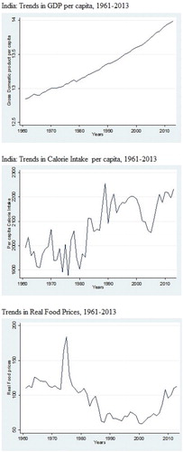
Figure 2. Scatter Plot; Calorie intake versus GDP, India, 1961–2013.

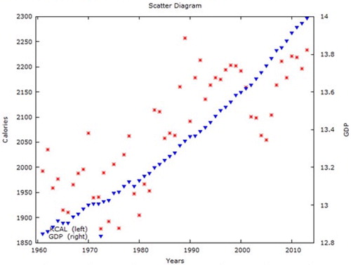
Table 1. Descriptive statistics.

Measures	GDP	KCAL	FP
Mean	13.33	3.32	1.96
Maximum	13.99	3.35	2.64
Minimum	12.84	3.32	1.77
Standard Deviation	0.33	0.02	0.11
Skewness	0.37	−0.20	0.15
Kurtosis	1.93	1.79	2.23

Note: The variables are in logarithmic transformation. Compilation Author.

Source: World Development Indicators, Pink Sheets Database World Bank. FAOSTAT (database).

Unit root tests

The variables used in this model are respectively GDP, KCAL and FP. Here the GDP indicates the natural logarithm of economic growth, KCAL indicates per capita nutritional intake in its natural logarithmic form and FP denotes the real food prices in its natural logarithmic form. Table 2 reports the unit root test of the series under observation based on the Augmented Dickey-Fuller unit root testing. From Table 2 it is observed that the series of the concerned variables are non-stationary at level but exhibit stationarity at first difference. Thus the series is both integrated of I (1). Unit root results presented in Table 3 are obtained from Zivot and Andrews (ZA), (2002) unit root test. This demonstrates a structural break endogenously in the series of observations. We find the same conclusions from the ZA test as obtained from the Dickey–Fuller test statistic. The series is stationary at I (1).

Table 2. Unit root tests, ADF.

Variables	Augmented Dickey- Fuller
At level
$KCAL$	−2.13
$GDP$	−2.838
FP	−1.86
At first difference
$\mathrm{\Delta }KCAL$	−10.12
$\mathrm{\Delta }GDP$	−9.768
$\mathrm{\Delta }$FP	−6.29
Notes: $\mathrm{\Delta }$ is the first difference term.
1% Critical	5% Critical	10% Critical (Dickey- Fuller)
Value	Value	Value
−4.224	−3.532	−3.199

Note: Lag lengths are selected based on the Akaike information criterion (AIC), Compilation Author.

Table 3. Zivot-Andrews unit root test.

Variables	Intercept			Trend			Both
	k	t	TB	k	t	TB	k	t	TB
KCAL	0	−4.41	1983	0	−4.24	1993	0	−4.63	1983
GDP	2	−2.02	1971	2	−2.69	1987	2	−3.04	1999
FP	2	−2.36	1982	2	−3.11	2001	2	−3.08	2000
ΔKCAL	0	−10.66*	1990	0	−10.19*	1980	0	−10.58*	1990
ΔGDP	2	−6.76*	1971	2	−6.57*	1973	2	−6.88*	2005
ΔFP	2	−9.54*	1976	2	−8.02*	1984	2	−9.69*	1979

Note: Δ indicates the variables in their first difference. The maximum lag length k is determined by the AIC criteria. T stands for the calculated test statistic. TB is the break in the time. *Indicates the test statistic is significant, so the rejection of the hypothesis that the series has a unit root. Compilation Author.

Cointegration test

Given that the variables economic growth, food prices and nutritional intake are integrated of order I (1), the cointegration test is run to obtain the long-run relation of the variables. Before conducting the Johansen procedure, hypothesis test process was conducted to select the order of the VAR, according to the AIC criteria, the lag length of 2 is chosen. The rank of the cointegrating vector is chosen following the trace and eigenvalue test.

The results of the Johansen cointegration test for both series are reported in Table 4. The results of the Johansen cointegration test (Table 4) show that the trace statistics and also the maximum eigenvalue statistics of the null hypothesis of no cointegration (r = 0) can be rejected in favor of the presence of at least one cointegrating equation. So the presence of cointegrating equation implies there exists a long-run relation between the variables. Therefore the standard Granger-causality test following equations (8), (9) and (10) is used to investigate the causality.

Table 4. Results of Johansen cointegration tests.

Null hypothesis	Trace statistic	Critical value
The number of cointegrating equation is zero (r = 0)	13.13	15.41
	Eigen value statistic	Critical value
	9.98	14.07
The number of co-integrating equation is at most one (r ≤ 1)	Trace statistic	Critical value
	3.14	3.76

Note: Compilation Author.

Table 5 presents the cointegration results for the three models (specification) of Gregory and Hansen (1996a, 1996b) with structural break. The estimation period runs from 1961 to 2013. The results, Table 5, are self-explanatory. Irrespective of the structural break all three models show a long-run cointegrating relation across calorie intake, GDP, and food prices.

Table 5. Results of the test for cointegration with structural breaks, Gregory Hansen method, (1961–2013).

Cointegration model	Break point	ADF* test statistic	Critical value			Rejection of H0 (Null) of No cointegration
			1%	5%	10%
Cointegration with Level Shift	2002	−5.82	−5.13	−4.61	−4.34	Yes
Cointegration with Level Shift and Trend	1994	−6.34	−5.45	−4.99	−4.72	Yes
Cointegration with Regime Shift	1989	−6.52	−5.47	−4.95	−4.68	Yes

Note: The critical values are from Gregory and Hansen (1996a).

Granger causality

Regressions (8), (9) and (10) were run to observe the short-run Granger causality. This test requires that per capita nutritional intake, are regressed on its own past values and past values of economic growth and real food prices. Similarly, economic growth is regressed on its own past values and past values of per capita nutritional intake and real food prices. Again real food prices are regressed on its own past values and past values of economic growth and nutritional intake. As evident from Table 6, there is a short-run causality running from economic growth towards nutritional intake in India. There is no causality running from nutritional intake to economic growth or food prices. A causality association exists from food prices to nutritional intake. The results, based on the Indian experience are in conformity with previous studies based in other developing countries, for example, are Dawson (2002) and Mushtaq, Gafoor, and Abeduallah (2007) for Pakistan; Halicioglu (2011) for Turkey; Ogundari (2011) for Nigeria. These country-based case studies conclude that there exists unidirectional causality association from economic growth to nutritional intake.

Table 6. Granger causality test results.

Direction of causality	F-value	Decision
GDP → KCAL	10.98(0.001)	Accept the direction of causality
GDP → FP	6.25 (0.53)	Reject the direction of causality
KCAL → GDP	0.14 (0.55)	Reject the direction of causality
KCAL → FP	1.23 (0.89)	Reject the direction of causality
FP → GDP	0.23 (0.76)	Reject the direction of causality
FP → KCAL	2.23 (0.006)	Accept the direction of causality

Note: Figure in the parenthesis indicated the probability at 5% level of significance. Compilation Author.

Variance decomposition and impulse response function

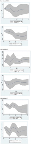
Table 7 provides the results for VDCS. During short time horizon, a major portion of the variance in calorie intake is explained by its own innovations. However, in the long-run, for example, when a 20 year period is considered the portion of the variance of calorie intake declines to 8.89%, implying the other variables, for example GDP, explain the shocks in calorie intake. For a 20 year time horizon, 68.09% of the shocks in calorie intake are due to innovations in GDP. So the post sample variance indicates that GDP is the main determinant of calorie intake. Halicioglu (2011) findings are similar to the observations made here.

Table 7. Generalized forecast error variance decomposition.

Time Horizons	KCAL	GDP	FP
The percentage of forecast variance explained by innovations in respective variables:
0	100.00	0	0
1	94.35	5.23	0.42
2	85.35	10.53	4.12
3	77.73	20.52	1.75
4	52.08	33.07	14.85
5	42.07	32.08	25.85
10	23.01	68.09	8.90
20	8.89	68.09	23.02

Note: Based on in sample observations: 1961–2013.

The impulse responses of calorie intake and the other variables are normalized to have a concomitant effect of one-percent change by dividing each shock by the standard deviation of the concerned variable. The basic method that is followed while calculating the impulse response function, setting the shocks to zero, then generating the simulation for all the variables up to the period where the impulse response is required.

The response of calorie to innovations in GDP is fluctuating. However, the response of GDP to the innovations of the calorie intake is converging to an equilibrium. Such observation is in line with Ganegodage, Taniguchi, and Wang (2003) findings for Sri Lanka. It is noticeable that at lower levels of economic growth the response of calorie intake to innovations in GDP is high. Thus this verifies Engel’s law which states that at lower levels of income countries spend a larger share of income on food items (Figure 3).

Figure 3. Impulse response functions to Cholesky one SD innovations.

The estimated model also undergoes a battery of diagnostic tests as reported in Table 8. Serial correlation is based on the Lagrange Multiplier test of residual; normality test is based on Skewness and Kurtosis of residuals and heteroscedasticity test is based on the regression of squared residuals on square fitted values. The null hypothesis of no serial correlation, no heteroscedasticity and normality of disturbance at the 5% level of significance cannot be rejected because the related p values are greater than 0.05%. Figure 4 plots roots of the companion matrix of stability of the concerned model.

Figure 4. Stability condition.

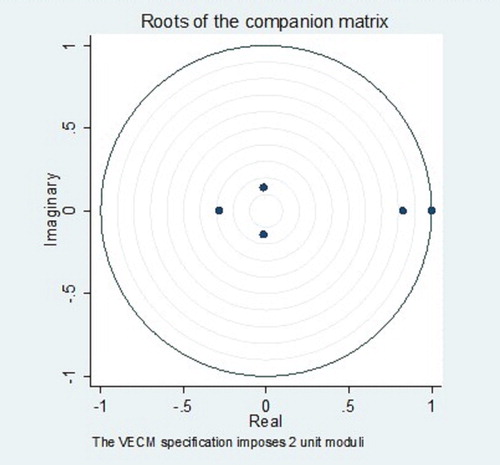
Table 8. Diagnostic test.

Diagnostic tests
Serial correlation	0.19
Heteroscedasticity	0.63
Normality	0.13

Policy implications

The existence of unidirectional causality from economic growth to nutritional intake in India establishes the hypothesis that a threshold level of income is required to ensure the proper dietary intake of the nation. Higher per capita availability of income implies individuals can afford a proper diet. However, the absence of direction of causality from dietary intake towards income implies that health does not manifest in the productivity of the nation.

The capability to be adequately nourished and live a strong healthy life organizes the foundation of leading a good life. Severe deficiencies in the aspects of health and nutrition are fundamentally unacceptable, particularly when they are insistent for certain disadvantaged groups of the population. The Indian experience is manifest with wide gaps in education and nutritional achievements across income quintiles, gender and across rural and urban populations. Faulty public expenditure policies, erroneous methods of service delivery and institutional constraints in terms of capacity building have played a significant role in expanding the health and nutritional inequalities in India. Operational policies to reduce income disparity are essential for the redistribution of wealth towards the poor, so they can effectively invest in health and nutritional offtake which would further invest in human capital formation. The formative steps could include raising the tax base of the rich. This can be accomplished by raising wealth tax and controlling the monopoly power of the landed aristocracy. Fiscal and monetary policies that are coherent with the inclusive growth can target low inflation and focus upon distributional inequalities in the area of health and education. Targeting a moderate inflation keeps the lending rates low, this, in turn, encourages investment, infuses growth thereby generating employment opportunities. Growing employment opportunities can in the long-run help in removing nutritional deficiencies, particularly among the marginalized population in India. Redistributive policy measures can provide households with consumer subsidies to allocate basic goods for their wellbeing. A minimum social security provided in the marginalized households will enable the households to invest in enhancing basic human capabilities like access to better health, education, and nutrition. The important programs for social assistance in India include conditional cash transfer programs, midday meal programs in schools and fee waivers. Consumer subsidy policies for self-targeted households in India are operational to remove the disparity in access to minimum calorie needs. The presentation of the National Food Security Act (NFSA) in August 2013 in India has changed the planning for food security and accordingly, the operation of Public Distribution System (PDS) became one of the most discussed subject matters in the country. PDS is one of the utmost significant public intervention programs to augment food security in India and therefore, the achievement of NFSA will judiciously rest on the proper functioning of PDS. PDS delivers a rationed quantity of essential food items and other non-food items at prices which are subsidized to consumers through a system of ‘fair price shops’. The scope and coverage of PDS has undergone several changes over the years, but it is fundamentally the mechanism to increase food security. With the enforcement of the system of Targeted Public Distribution System (TPDS) in 1997, the aim is to target the poorest households, so that they are allowed to buy the rationed items from the fair price shops. However, continuing malpractices in the system still present considerable difficulties which need to be addressed from time to time. The ‘Food Security Allowance Rules, 2015’ were reported by the Central Government on 21 January 2015, and postulate the standards for calculating and paying the allowance that the targeted households are entitled to. Moreover, raising agricultural productivity for a developing country like India is important for improving income levels in poor households. Improved access to infrastructure and market services can enable farmers to translate their produce to larger incomes. However, legislative reforms pertaining to land distribution are the foremost strategy to remove inequalities in income which would translate into better quality living. The state needs to ensure equal opportunity for all its members in participation in the universal public provisioning of essential social services. Organizing community participation of the deprived sections for addressing their grievances in public meetings would make the service providers more transparent and accountable.

Policies encouraging participatory community-based programs can be beneficial in the long-run to remove inequality in access towards better health and human capital formation. Families and communities are commonly able to assess, explore, and take action to remove certain bottlenecks in the delivery of services related to human capital formation. Communities can generate a sense of accountability among the clientele. Mechanisms such as a social audit can make the government of India further accountable to its citizens. Citizen report cards and documentation of feedback surveys will raise the responsibility of service providers and remove malpractices in the delivery mechanism. The provision of widespread appropriate health and nutrition services must be the crucial element of a socially all-encompassing development program, and policy focus should aim at finding connections across undernutrition and numerous deficiencies related to poverty, exclusion, and gender bias. The Seventh Five Year Plan in India has acknowledged the importance of human resource development in accelerating the process of economic growth and to bring about desirable social change. Investment in human resources includes the development of educational access for the population particularly the marginalized section. There is a need for a shift in emphasis of the education policy plan from enrollment to upgrading the working of schools as well as towards fostering the quality of education. The social and cultural hurdles which hamper active participation in the process of learning should be effectively tackled. The illiterate population of India is largely concentrated in seven states, the endeavor should be to reach out to these states through a quality schooling process. A school mapping process would benefit to ensure equitable access not only at the primary level, but also at the upper primary level. The government of India needs to set up long-term goals to plug gender gaps in the availability of schools at the higher levels. Human capital formation is not just about acquiring skills and studying it also needs to ensure the health and nutritional status of students. Malnutrition restricts the ability to learn by severely affecting the sensory, motor, and cognitive expansion of students. Here, it is necessary to address the issue of education with other related development aspects, particularly in the areas of health for the sustainable development of human capital. Provision of District Health Action Plans and the mapping of people’s health needs on the basis of habitation can generate decentralization in health delivery as well as make a more accountable system. The prime focus of the public health policy should be tackling preventable and communicable diseases, by providing clean water and sanitation methods. However, given the vastness of the country, India still faces severe challenges in health care. The public expenditure on health care needs to expand to enable the poor to have access to quality health services. In order to fight malnutrition, it is essential to endorse policies that would raise the food productivity together with improving the cropping pattern. The multi-dimensional nature of the malnutrition problem necessitates the convergence of many schemes related to health, education, water, and sanitation with food security. The setting up of the National Nutrition Mission can help the states fight malnutrition, once the states put forward their plans to participate in the mission. Last, social mobilization is an effective instrument in India for achieving the desired nutritional objectives. This can be attained by involving people in educating the community about the importance of nutrition and the governmental processes involved in it.

India needs to develop data collection processes which will address the causes and consequences of nutritional deficiencies. Educating households on the nutritional value of food through labeling of nutritional information can be periodically assessed to see whether it is generating adequate educational information among households. The primary causes of India’s ‘malnutrition’ are more complicated and go beyond direct nutritional input needs. For example, 50% of malnutrition cases are associated with chronic diarrhoea caused by the lack of clean water, sanitation, and hygiene and unhealthy practices such as open defecation which makes children susceptible to infections. The present endeavor of the government under the Swachh Bharat Abhiyan will go a long way towards combatting communicable disease through the construction of toilets.

It must be pointed out that the policy suggestions developed out of this research are limited owing to the utilization of aggregate data for analysis. The institutional and organizational details explaining the calorie intake and income growth nexus often do not receive proper representation. More detailed nutritional guidelines should be prepared by the Ministry of Human Resource Development, Government of India to target the varied segments of the population so that the efficiency of the measures are optimized.

Conclusion

This study has tested the long-run relationship between per capita calorie intake, per GDP and real food prices for India during 1961–2013 using the Johansen and Juselius (1990) method to cointegration. The results of this paper are in conformity with previous empirical research based on other developing countries in the Asia region. The study demonstrates that there exists a statistically significant long-run relation between nutritional intake and economic growth. The impact of real food prices on calorie intake is significant in the short-run. The Granger-causality test confirms a unidirectional causal association from income growth to nutritional intake. So rising incomes in India can subsequently reduce the insufficient intake of calories. The variance decomposition analysis also confirms that income growth is a significant determinant of calorie intake in the long-run. The impulse response functions show the short-run causation of interactions among variables, here also GDP is a major explanatory variable for calorie intake.

Disclosure statement

No potential conflict of interest was reported by the authors.

ORCID

Sudeshna Ghosh http://orcid.org/0000-0002-2026-1676

References

- Ahluwalia, Montek Singh. 2002. “State Level Performance Under Economic Reforms in India.” In Economic Policy Reforms and the Indian Economy, edited by Anne O. Krueger, 91–125. Chicago: Chicago Press.
- Ahluwalia, Montek Singh. 2011. “Prospects and Policy Challenges in the Twelfth Plan.” Economic and Political Weekly 46 (21): 88–105.
- Arcand, Jean Louis. 2001. “Undernourishment and Economic Growth: The Efficiency Cost of Hunger.” (No. 147). Food & Agriculture Org.
- Banerjee, Abhijit V., and Esther Duflo. 2011. “More Than 1 Billion People are Hungry in the World.” Foreign Policy 186: 66–72.
- Basu, Deepankar, and Amit Basole. 2012. “The Calorie Consumption Puzzle in India: An Empirical Investigation.” (No. 2012-07). Working Paper, University of Massachusetts, Department of Economics.
- Bhargava, Alok. 2001. “Nutrition, Health, and Economic Development: Some Policy Priorities.” Food and Nutrition Bulletin 22 (2): 173–177.
- Brown, Stephen P. A., Mine K. Yucel, and John Thompson. 2004. “Business Cycles: The Role of Energy Prices.” Research Department Working Paper, 0304, Federal Reserve Bank of Dallas. Accessed January 14, 2018. https://core.ac.uk/download/pdf/7359279.pdf.
- Cole, William E. 1971. “Investment in Nutrition as a Factor in the Economic Growth of Developing Countries.” Land Economics 47 (2): 139–149.
- Dawson, Philip J. 2002. “Nutrition in Pakistan: Estimating the Economic Demand for Calories.” Pakistan Journal of Nutrition 1 (1): 64–66.
- Dawson, Philip J., and Ana I. Sanjuán. 2011. “Calorie Consumption and Income: Panel Cointegration and Causality Evidence in Developing Countries.” Applied Economics Letters 18 (15): 1455–1461.
- Deaton, Angus, and Jean Dreze. 2008. “Nutrition in India: Facts and Interpretations.” Economic and Political Weekly 44 (7): 42–65.
- Dickey, David A., and Wayne A. Fuller. 1979. “Distribution of the Estimators for Autoregressive Time Series with a Unit Root.” Journal of the American Statistical Association 74 (366a): 427–431.
- Food Agriculture Organization of the United Nations Statistics Division (FAOSTAT database) [Online]. Accessed August 1, 2017. http://faostat.fao.org/default.aspx.
- Ganegodage, Renuka, Kiyoshi Taniguchi, and Xiaojun Wang. 2003. “Learning by Eating: A Case Study on the Cost of Hunger in Sri Lanka.” ESA Working Paper No. 03-05. Agriculture and Economic Development Analysis Division. The Food and Agriculture Organization of the United Nations.
- Golait, Ramesh, and Narayan C. Pradhan. 2006. “Changing Food Consumption Pattern in Rural India: Implication on Food and Nutrition Security.” Indian Journal of Agricultural Economics 61 (3): 374–388.
- Gregory, A. W., and B. E. Hansen. 1996a. “Residual-based Tests for Cointegration in Models with Regime Shifts.” Journal of Econometrics 70 (1): 99–126.
- Gregory, A. W., and B. E. Hansen. 1996b. “Tests for Cointegration in Models With Regime and Trend Shifts.” Oxford Bulletin of Economics and Statistics 58 (3): 555–560.
- Gujarati, Damodar N. 2009. Basic Econometrics. New Delhi: Tata McGraw-Hill Education.
- Halicioglu, Ferda. 2011. “The Demand for Calories in Turkey.” Accessed July 30, 2017. https://mpra.ub.uni-muenchen.de/41807/.
- Hartwig, Jochen. 2010. “Is Health Capital Formation Good for Long-Term Economic Growth?–Panel Granger-Causality Evidence for OECD Countries.” Journal of Macroeconomics 32 (1): 314–325.
- Johansen, Soren, and Katarina Juselius. 1990. “Maximum Likelihood Estimation and Inference on Cointegration—With Applications to the Demand for Money.” Oxford Bulletin of Economics and Statistics 52 (2): 169–210.
- Landy, Frederic. 2009. “India, ‘Cultural Density’ and the Model of Food Transition.” Economic and Political Weekly 44 (20): 59–61.
- Malik, Garima. 2006. “An Examination of the Relationship Between Health and Economic Growth.” Working Paper No.185. Indian Council For Research On International EconomicRelations, Accessed July 30, 2017. http://www.eaber.org/sites/default/files/documents/ICRIER_Malik_2006.pdf.
- Mushtaq, Khalid, Abdul Gafoor, and Abeduallah. 2007. “An Examination of Calorie Demand Relationship in Pakistan.” Pakistan Journal of Nutrition 6 (2): 159–162.
- National Nutrition Monitoring Bureau. 2005. Assessment of Diet and Nutritional Status of Individuals and Prevalence of Hypertension in Adults & Anemia among Men and NPNL Women in Rural Communities. Hyderabad: National Institute of Nutrition.
- Neeliah, Harris, and Bhavani Shankar. 2008. “Is Nutritional Improvement a Cause or a Consequence of Economic Growth? Evidence from Mauritius.” Economics Bulletin 17 (8): 1–11.
- Ogundari, Kolawole. 2011. “Estimating Demand for Nutrients in Nigeria: A Vector Error-Correction Model.” MPRA Papers, No. 28930.
- Papola, T. S. 2012. “Structural Changes In the Indian Economy, Emerging Patterns and Implications.” Institute for Studies in Industrial Development, Working Paper, 2012/02. Accessed January 18, 2018. http://isidev.nic.in/pdf/WP1202.pdf.
- Patnaik, Utsa. 2007. “Neoliberalism and Rural Poverty in India.” Economic and Political Weekly 42 (30): 3132–3150.
- Radhakrishna, R. 2012. Food Consumption and Nutritional Status in India: Emerging Trends and Perspectives. Mumbai: Indira Gandhi Institute of Development Research. Accessed January 14, 2018. http://www.igidr.ac.in/pdf/publication/WP-2006-008.pdf.
- Seddighi, Hamid, Kevin Lawler, and Anastasios V. Katos. 2000. Econometrics: A Practical Approach. London: Routledge.
- Sims, Christopher A. 1980. “Macroeconomics and Reality.” Econometrica 48 (1): 1–48.
- Smith, Lisa C. 2015. “The Great Indian Calorie Debate: Explaining Rising Undernourishment During India’s Rapid Economic Growth.” Food Policy 50: 53–67.
- Spurr, G. B. 1983. “Nutritional Status and Physical Work Capacity.” American Journal of Physical Anthropology, 26 (S1): 1–35. doi:10.1002/ajpa.1330260503.
- Stock, James H., and Mark W. Watson. 1989. “Interpreting the Evidence on Money-Income Causality.” Journal of Econometrics 40 (1): 161–181.
- Strauss, John S., and Duncan Thomas. 1998. “Health, Nutrition, and Economic Development.” Journal of Economic Literature 36 (2): 766–817.
- Tiffin, Richard, and P. J. Dawson. 2002. “The Demand for Calories: Some Further Estimates from Zimbabwe.” Journal of Agricultural Economics 53 (2): 221–232.
- Wang, X., and K. Taniguchi. 2003. “Does Better Nutrition Enhance Economic Growth? The Economic Cost of Hunger.” In Nutrition Intake and Economic Growth. Studies on the Cost of Hunger, edited by K. Taniguchi and X. Wang. Rome: FAO. http://www.fao.org/docrep/006/y4850e/y4850e04.htm.
- World Bank. 2014. “South Asia Economic Focus.” The Export Opportunity. Accessed January 14, 2018. http://www.worldbank.org/content/dam/Worldbank/document/SAR/south-asia-economic-focus-export-opportunity.pdf.
- World Bank. 2015. India Country Snapshot. Accessed January 12, 2017. http://documents.worldbank.org/curated/en/971731467998752846/India-Country-snapshot.
- World Bank. Commodity Price Data: Pink Sheet. Washington, DC: Development Prospects Group. Various Issues. Accessed January 11, 2017. http://blogs.worldbank.org/prospects/category/tags/historical-data.
- World Development Indicators; World Bank database [Online]. Accessed August 1, 2017. http://devdata.worldbank.org/dataonline.
- Zivot, Eric, and Donald W. K. Andrews. 2002. “Further Evidence on the Great Crash, the Oil-Price Shock, and the Unit-Root Hypothesis.” Journal of Business & Economic Statistics 20 (1): 25–44.