Can unconditional cash assistance improve household welfare? QUAIDS model for food commodities in Indonesia

ABSTRACT

Expenditure patterns can be taken into consideration in determining the type of government assistance. Without adequate information on household expenditure patterns, cash transfers may not be effective in improving welfare. This study aims to examine the expenditure patterns of households receiving cash assistance in Indonesia. The expenditure pattern is estimated using the Quadratic Almost Ideal Demand System (QUAIDS). Four groups of expenditure types for food were examined: rice, staple food, beverages, tobacco and alcoholic beverages. The result showed that the largest predicted expenditure is for the purchase of staple food. Income elasticity for staple food is relatively highest than all other types of food. On the other hand, the price elasticity of tobacco and alcoholic beverages is relatively inelastic (lowest) compared to other food products. These results indicate that the provision of cash transfers for poor households has the potential to increase household welfare through increasing staple food consumption.

KEYWORDS:

• Expenditure pattern
• food commodities
• cash transfer
• elasticity

JEL CLASSIFICATIONS:

• D12
• O13
• Q11

Introduction

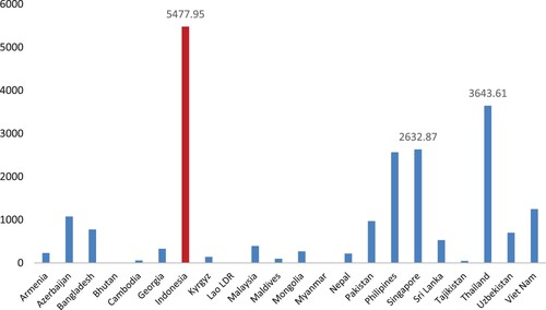
The pattern of household consumption expenditure is very important information to determine household preferences for basic goods. This information can be used to evaluate the effectiveness of cash assistance provided by the government for improving welfare of receiving household. Indonesia is one of the countries that provide much social assistance, including cash transfers. Based on data from the Asian Development Bank, expenditure on social assistance in Indonesia in 2015 was the highest in the Asia Pacific region excluding China, Japan, and the Republic of Korea (Asian Development Bank 2019). Indonesia’s Expenditure for social assistance in 2015 was $5477.95 followed by Thailand ($3643.61) and Singapore ($2632.87) (Figure 1).

Figure 1. Social assistance expenditure by country, 2015 ($ million). Source: The Sosial Protection Indicator for Asia, Asian Development Bank 2019.

One form of social assistance provided by the government is in the form of unconditional cash transfers. Beneficiary households are free to use cash assistance for any purpose according to their preferences (Aung et al. 2021; Handa et al. 2018). Many studies have been conducted to examine the impact of cash transfers on household welfare. The welfare aspect that is analysed involves economic condition (Haushofer and Shapiro 2016), happiness (Natali et al. 2018) to health problems (Hjelm et al. 2017). However, studies on the impact of providing cash transfers by the government have so far not been linked to the expenditure patterns of beneficiary households. The pattern of household expenditure can be used as an initial source of information about the types of goods that will be spent if certain households receive additional cash. Therefore, studies on the impact of cash transfers should also pay attention to this important aspect.

The pattern of food consumption expenditure can be evaluated using a system of demand equations. One of the popular demand equation system models used in empirical studies is the Almost Ideal Demand System (AIDS) approach. This model can be estimated using a system of linear equations (Sheng et al. 2008) or a system of quadratic equations (Elzaki, Yunus Sisman, and Al-Mahish 2021). Currently, more flexible estimation techniques have been developed to estimate linear and quadratic models simultaneously (Poi 2008). This technique can also be expanded by explicitly adding demographic elements to the model. The model system of equations is then known as the Quadratic Almost Demand System (QUAIDS) which is used as the basis of analysis in this study.

As already mentioned, Indonesia is one of the countries that provide much assistance in the form of cash transfers. It is recorded that since 2005, about eight times this model of unconditional transfer was launched by the government to anticipate economic turmoil. In 2005–2006 the provision of cash assistance was intended to anticipate the decline in consumption due to the increase in world oil prices (SMERU 2006). Furthermore, in 2008–2009 the government provided cash assistance due to the world recession. The weakening of the world economy (2013–2015) was also used as a reason for the government to provide similar assistance (World Bank 2017). The distribution of cash assistance was also provided by the government to anticipate the economic downturn due to the COVID-19 pandemic in 2020 (Barany et al. 2020). In mid-2021, the Indonesian government also issued cash assistance as compensation for the policy of restricting community activities to reduce the spread of the coronavirus. There are around 15 million households receiving cash transfer assistance in Indonesia.

The relatively high intensity of cash transfer distribution with a large target of recipient households has motivated researchers to evaluate the spending patterns of beneficiary households. The specific research objectives are: (1) determining the share of household expenditure for various types of food; (2) estimating the income elasticity of the types of food products studied; (3) estimating the price elasticity of each food product under study.

The outline of this paper is structured as follows. The introductory session explained the background, motivation and objectives of the research. The literature review session discussed the basic concepts of demand and previous research relevant to the topic of food demand. The methodology session discussed research data, analytical models and estimation techniques used. The result and discussion session explained the results of the research as well as discussions related to the results of the research. This paper closes with a session of conclusions and policy implications.

Literature review

In the microeconomic literature, individual demand can be expressed in terms of direct utility function and indirect utility function (Moffatt 2012). The development of a demand model consisting of several types of commodities is realized in the estimation of a system of equations model. One model of the system of equations that is popularly used today is the Al-most Ideal Demand System (AIDS) which was originally proposed by Banks, Blundell, and Lewbel (1997).

This model begins with an indirect utility function which is formulated as follows: (1) $\ln V(p,m)={\left[{\left\{{\displaystyle \frac{\ln m-\ln a(p)}{\ln b(p)}}\right\}}^{-1}+\lambda (p)\right]}^{-1}$(1) In this case $\ln a(p)$ is a function of the transcendental logarithm. The variables p and m are the price level and total expenditure, respectively. Following Deaton and Muellbauer (1980), the parameterization of the above demand variable is stated as follows (Labandeira, Labeaga, and Rodríguez 2006): (2) $\ln a(p)={\alpha }_0+\sum _{i=1}^k{\alpha }_i\ln p_i+{\displaystyle \frac{1}{2}\sum _{i=1}^k\sum _{j=1}^k{\gamma }_{ij}\ln p_i\ln p_k}$(2) The function above shows that $p_i$ is the price of goods i for i =  1 …  … k. Meanwhile b(p) is a price aggregator of the Cobb–Douglas type. The last fractions of the indirect utility functions in equation (1) are as follows: (3) $b(p)=\prod _{i=k}^k{p}_i^{{\beta }_i}$(3) and definition: (4) $\lambda (p)=\sum _{i=k}^k{\lambda }_i\ln p_i$(4) The assumptions used in the AIDS model are adding up, homogeneity and Slutsky symmetry which can be expressed as follows (Poi 2012): (5) $\sum _{i=1}^k{\alpha }_i=1,\sum _{i=1}^k{\beta }_i=0,\sum _{j=1}^k{\gamma }_{ij}=0,\sum _{i=1}^k{\lambda }_i=0,{\gamma }_{ij}={\gamma }_{ij}$(5) By using Roy’s Identity principle, from equation (1), the budget share equation will be obtained as follows: (6) $w_i={\alpha }_i+\sum _{j=k}^k{\gamma }_{ij}\ln p_j+{\beta }_i\ln \left\{{\displaystyle \frac{m}{a(p)}}\right\},i=1,\dots k$(6) In this case $w_i$ is the portion of consumption expenditure and $p_j$ is the price level for the commodity in question. Meanwhile, m is the total household expenditure. Equation (6) is the basic model of AIDS whose coefficient will be estimated empirically.

The application of the AIDS approach to estimating household behavior in managing expenditure has been widely carried out in several countries. The case in Mexico specifically evaluates changes in income elasticity, price elasticity and value of food waste before and during COVID-19 (Vargas-Lopez et al. 2021). This study uses a survey approach to respondents obtained from social media. In general, it was found that COVID-19 brought changes in people’s behavior in consuming food during the pandemic. The survey that was conducted did not specifically divide the respondents according to certain socioeconomic classes.

Research on household consumption patterns with fairly representative data nationally was conducted in Ghana (Ansah, Marfo, and Donkoh 2020). The types of food commodities studied are quite complex (there are about 14 types of food). The results showed that very poor households had a larger share of food expenditure compared to other household groups. Therefore, food-related policies need to be directed at very poor households.

Research on income elasticity for food in Africa is relatively much done so that Colen et al. (2018) conducted a meta-analysis on this topic. Gathering a total of 66 primary studies from 48 African countries, the study reports unique findings. Although an increase in income will encourage an increase in food consumption, the increase is mostly in the form of fat and sugar intake. For this reason, anti-poverty policies still need to be carried out but recipients of assistance must also be made aware of the importance of health aspects in consuming.

Furthermore, research that is special in nature, with a more limited object of food is carried out with an experimental approach (Conrad, Jahns, and Roemmich 2018). This study divides the respondents into two groups, namely program recipients and non-program recipients. The results of the study show that changes in food commodity prices will have a very large effect on the purchase of certain commodities. Just like previous research, this research suggests the need for education about food health for low-income households.

Based on the discussion in the literature review, several important points can be underlined. First, the AIDS approach is the main tool in estimating the food demand system in a country. Second, research on consumption behavior is still general in nature, rarely focusing on households with lower middle income. Third, research on consumption patterns has not yet been linked to the behavior of beneficiary households. Fourth, awareness to promote healthy living is getting stronger along with the many findings related to household’s behavior in consumption.

To fill the research gap that is still rarely done, the research was conducted with a focus on poor households receiving government assistance. It is hoped that through this research, the policy of unconditional cash transfers must be considered again for its effectiveness in improving the quality of life of beneficiary households.

Methodology

The basic AIDS model in equation (6) is expanded so that it becomes a quadratic form as follows: (7) $w_i={\alpha }_i+\sum _{j=k}^k{\gamma }_{ij}\ln p_j+{\beta }_i\ln \left\{{\displaystyle \frac{m}{a(p)}}\right\}+{\displaystyle \frac{{\lambda }_i}{b(p)}{\left[\ln \left\{{\displaystyle \frac{m}{a(p)}}\right\}\right]}^2}$(7) The model in equation (7) is known as the Quadratic Almost Ideal Demand System (QUAIDS) which is nothing but a quadratic version of the linear AIDS basic equation model in equation (6). Technically there are four groups of coefficients that must be estimated, namely alpha (α), beta (β), gamma (γ) and lambda (λ). The lambda coefficient is a specific coefficient for QUAIDS, if this coefficient is not significant then the AIDS linear model is more appropriate to be chosen. Therefore, the critical coefficients in this model are beta and gamma.

The estimation of the coefficients of the equation (6) can be carried out using several estimation techniques. The most basic technique is to use the Ordinary Least Square (OLS) partially for each commodity separately. This basic estimation method (OLS) is very inefficient because it must estimate one by one. In addition, this method ignores the possibility of a correlation between error terms between equations. If this kind of correlation is strong enough, then the results of the OLS estimation are potentially biased. To overcome this problem, researchers prefer systemic estimation techniques. Labandeira, Labeaga, and Rodríguez (2006), chose the Instrumental Variables (IV) technique with two stages. A similar estimation technique but with a slightly different version was carried out by Li and Just (2018) with Two Step Limited Information Maximum Likelihood.

In addition to different estimation techniques, demand system equations are also carried out with various reference estimation models. Nganau (2011) uses the Linear Expenditure System (LES) approach to estimate the economic system in Africa. The quadratic version of the LES was used by Schulte and Heindl (2016) to estimate demand behavior in Germany. Although most of the demand equation system research uses individual/household micro data, some researchers also use aggregated data techniques with a very long research period (Kratena and Wüger 2010).

The various models, estimation techniques and data used by researchers each have advantages and disadvantages. In principle, a more flexible model accompanied by an estimation technique that is relatively easy to implement will be chosen in this study. Based on these considerations, in this study the QUAIDS approach was chosen which was introduced by Poi (2012). In this approach, parameter estimation is performed using the Feasible Generalized Non-Linear Estimation method. As an alternative, the estimation of AIDS model parameters in this study was also carried out using an Iterative Linear Least Square approach (Lecocq and Robin 2015). The Iterative Linear Least Square approach is relatively simple and can produce individual equation estimates. The choice of using the Generalized Least Square (GLS) or Linear Least Square (LLS) approach is strongly influenced by the error term distribution of each equation (Hansen 2007). This issue will be discussed in the results section of the study.

Parameter estimation in QUAIDS is the initial stage of the data analysis process. In empirical research, the information needed is not only the significance of the coefficient but also the income elasticity coefficient and price elasticity of each commodity. Fortunately, the Poi (2012) approach in STATA already has sufficient facilities to provide post-estimated information. The postestimation information provided includes, among others; prediction of share of expenditure for each commodity, income elasticity, compensated price elasticity and uncompensated price elasticity. Price elasticity is displayed not only in the form of own price elasticity, but also cross price elasticity.

The income elasticity is obtained from the differentiation equation (6) with respect to total expenditure: (8) ${\mu }_i=1+{\displaystyle \frac{{\beta }_i}{w_i}}$(8) Furthermore, Marshallian price elasticity is obtained from differentiation equation (6) respect to price of good: (9) $e_i^m={\displaystyle \frac{1}{w_i}\left[{\gamma }_{ij}-{\beta }_i\left({\alpha }_i+\sum _{j=k}^k{\gamma }_{ij}\ln p_j\right)\right]}$(9) The Hicksian price elasticity can be obtained through the Slutsky equation as follows: (10) $e_i^h=e_i^m+{\mu }_i{w}_i$(10) The estimates of income elasticity and price elasticity in equation (8) and equation (9) are linear derivatives of AIDS. The formula for the QUAIDS version can be referenced in Poi (2012).

The data used in this study is sourced from the fifth wave of the Indonesia Family Life Survey (IFLS) data (IFLS-5) which was published in 2016. The IFLS data series is actually a relatively representative household panel data. Starting in 1993 (IFLS-1), the latest data updates are released regularly every seven years. In 1998, a specific survey version was re-leased to accommodate changes in data behavior due to the current eco-nomic turmoil (IFLS-2). Subsequently, in 2000, the 3rd wave of IFLS data update (IFLS-3) was published. Seven years later, namely in 2007, the fourth series of IFLS data (IFLS-4) was published. Finally, in 2014 the fifth wave of IFLS update data was released (Strauss, Witoelar, and Sikoki 2016).

IFLS data includes all information related to household activities in Indonesia. Based on available information, IFLS data represent 80% of the total population covering 13 provinces in Indonesia. The surveyed households in the first release were around 7000 households and continued to grow until they reached about 15,000 households in the last data release. The information provided in IFLS is quite complex, starting from consumption expenditure data, health information, education level, welfare, farming, non-agricultural business, nutritional status of women and children, decision making, sleep quality and so on. Interestingly, this micro data consists of several levels of unit of analysis ranging from individuals, households to communities. This relatively complete facility encourages a lot of research that uses this data as a basis for analysis (Rasyid et al. 2020).

Regarding household consumption, IFLS has provided quite abundant information regarding the expenditure of various types of commodities ranging from food, health, recreation to expenditure for transfers. In accordance with the purpose of the study, the household data chosen to be used as the basis for the research were households that received cash assistance from the government. The types of consumption goods analysed consisted of four groups of goods, namely rice, other staple foods, bever-ages and expenditures on tobacco and alcohol. This type of expenditure was chosen according to the purpose of the study.

The results of the IFLS-5 data search show that the total number of households that were successfully interviewed were 15,134 households. Of the total households, around 11.89% were households that received unconditional cash transfers in 2014. After further data cleaning and removing a number of missing observations, 1779 households were collected which were used as the basis for analysis. Households collected as a sample are representative of the household population in Indonesia. Based on data from the Indonesian Central Statistics Agency in 2013, the pattern of household consumption expenditure is as follows: expenditure on rice by 21.9%; expenditure on other staple foods by 30.2%; consumption of various beverages as much as 15.3%; tobacco as much as 24.2% and other expenses by 8.4% (BPS 2013). This pattern is relatively similar to the IFLS household consumption pattern: 25% for rice; staple foods 32%; various beverages 14% and tobacco/alcohol 28%.

Result and discussion

The data used in this study includes information on consumption expenditures of more than 1700 households in Indonesia. The research variables consist of the portion of expenditure, the price of each commodity and the total household expenditure.

Table 1 presents descriptive statistics of the variables used in this study. The number of households that were sampled was 1779 households. The number of variables used is 9 variables consisting of three groups of variables: the variable portion of expenditure, the variable price of food items and the total household expenditure. The type of household expenditure studied consisted of expenditure on rice, expenditure on other staple foods, expenditure on beverages and expenditure on tobacco and alcoholic beverages.

Table 1. Summary statistic of data.

Variables	Obs.	Mean	Std. Dev
Share of rice (%)	1779	0.2511	0.1840
Share of staple (%)	1779	0.3220	0.1942
Share of beverages (%)	1779	0.1422	0.2145
Share of tobacco/alc. (%)	1779	0.2847	0.2974
Price of rice (Rp)	1779	61,529	7,600
Price of staple (Rp)	1779	68,639	7,345
Price of beverages (Rp)	1779	14,598	1,967
Price of tobacco/alc. (Rp)	1779	46,681	6,599
Expenditure/Bugdet (Rp)	1779	780,099	70,726

Source: Author calculation.

The expenditure portion data for each commodity group is expressed in the form of a percentage. As can be seen in Table 1, the largest expenditure of cash transfer recipient households is for basic necessities. Expenditure on rice reached 25% and expenditure on other basic commodities reached 32%. These results indicate that about 57% of household expenditures for beneficiaries are in the form of staple foods. Furthermore, the other largest expenditure group is for tobacco and alcoholic beverages. On average, total household expenditure on this commodity reaches around 28%. The remaining expenses are used for the purchase of beverages.

Following Banks, Blundell, and Lewbel (1997), before estimating the parameters of the AIDS model, it is necessary to plot the consumption portion of each commodity group and the total expenditure. This plotting is carried out using two techniques, namely Local Linear Smoothing (LOWESS) and Fractional-Polynomial Prediction Plot. The plotting results can be seen in Figure 2 as follows:

Figure 2. (A) Plotting predicted share of rice and household budget; (B) plotting predicted share of staple food and household budget; (C) Plotting predicted share of beverages and household budget; (D) Plotting predicted share of Tobacco/Alc. beverages and household budget.

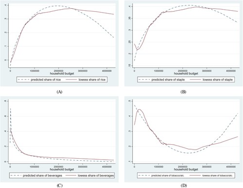
The results of plotting each share of household consumption on total expenditure or household budget produce different patterns. The consumption pattern of rice and staple food forms an inverted-U curve (Figure 2(A,B)). At low-income levels, the share of rice and staple food increases. However, at the middle-income level, the share for both types of goods decreased. Consumption patterns for beverages are decreasing along with higher incomes. The higher the expenditure, the lower the rate of decline in consumption for beverages (Figure 2(C)). Furthermore, the pattern of consumption of cigarettes and alcoholic beverages has a different pattern (Figure 2(D)). At low expenditure levels, the share for cigarettes and alcoholic beverages decreases. However, when income reaches the middle level, the portion of consumption for cigarettes and alcoholic beverages increases (U-shaped). Based on the basic plotting, it is found that the non-linear model is relatively more able to describe household consumption patterns. In this research, the chosen non-linear model is quadratic. Tests on the significance of the quadratic model in more detail will be discussed later.

The results of QUAIDS estimation using the Generalized Least Square (Poi 2012) and Iterative Least Square (Lecocq and Robin 2015) approaches can be shown in Table 2 as follows:

Table 2. Result of QUAIDS estimation: GLS approach.

	Rice		Staple		Beverages		Tobacco/Alc.
	Coef.	SE	Coef.	SE	Coef.	SE	Coef.	SE
Constant	0.264	0.002	0.260	0.003	0.092	0.003	0.385	0.004
Price Rice	0.024	0.000	−0.004	0.000	−0.006	0.000	−0.014	0.000
Price Staple	−0.004	0.000	0.031	0.001	−0.010	0.000	−0.018	0.000
Price Beverage	−0.006	0.000	−0.010	0.000	0.020	0.001	−0.004	0.000
Prices Tbc/Alc.	−0.014	0.000	−0.018	0.000	−0.004	0.000	0.036	0.001
Expenditure	−0.027	0.001	−0.025	0.002	0.009	0.002	0.044	0.003
Expenditure Sqrt	−0.003	0.000	0.001	0.001	0.021	0.000	−0.020	0.001

The QUAIDS model for four groups of commodity types requires estimation of 28 parameters. Table 2 presents the estimation results of quadratic AIDS using Generalized Least Square, while Table 3 presents the estimation results of the same model using Iterative Least Square. At a glance, it can be shown that all the estimated coefficients are significant at the conventional level (5%). The results showed that all expenditure square coefficients were partially significant. Joint estimation testing for that coefficient also resulted in the conclusion quadratic coefficient was significantly different from zero. Given that the expenditure square coefficient is a characteristic of the quadratic element of equation (7) it can be concluded that the quadratic AIDS model is statistically proven to be superior to the linear AIDS model.

Table 3. Result of QUAIDS estimation: ILS approach.

	Rice		Staple		Beverages		Tobacco/Alc.
	Coef.	SE	Coef.	SE	Coef.	SE	Coef.	SE
Constant	0.207	0.005	0.223	0.009	0.137	0.009	0.433	0.012
Price Rice	0.028	0.000	0.003	0.001	−0.011	0.001	−0.020	0.001
Price Staple	−0.003	0.001	0.028	0.001	−0.007	0.001	−0.018	0.001
Price Beverage	−0.005	0.000	−0.010	0.001	0.019	0.001	−0.004	0.001
Prices Tbc/Alc.	−0.012	0.000	−0.014	0.001	−0.007	0.001	0.033	0.001
Expenditure	−0.014	0.002	0.004	0.003	−0.007	0.004	0.018	0.004
Expenditure Sqrt	−0.003	0.000	−0.002	0.001	0.022	0.001	−0.017	0.001

Before analysing the estimation results, a test of the residual behavior is carried out in each equation. Residual tests used in this study were the Portmanteau test (white noise process) and the Shapiro–Wilk test (normality). The test results are summarized in Table 4 as follows:

Table 4. Residual test and joint quadratic coefficient test.

White Noise Process
Equation	Portmanteau (Q) Statistic	Prob > Chi2
Rice (w1)	32.4187	0.7973
Staple (w2)	43.8606	0.3112
Beverages (w3)	50.3437	0.1266
Tobacco/Alc. (w4)	53.3537	0.0769
Normality Test
Equation	Shapiro-Wilk (z) Statistic	Prob > z
Rice (w1)	0.342	0.36601
Staple (w2)	0.225	0.41116
Beverages (w3)	0.688	0.24584
Tobacco/Alc. (w4)	0.705	0.24031
Joint Quadratic Coefficient Test
	GLS	ILS
Chi2 (3)	2725.65	1636.71
Prob > Chi2	0.0000	0.0000

 Source: STATA Output.

The results of the residual test in Table 4 show that all of the estimated equations have met the conditions of the white noise process and the assumption of normality. At the end of Table 4, the results of the simultaneous quadratic coefficient significance test for each approach are also included. The test results show that the quadratic model is more suitable than the linear model.

Estimating the parameters of the QUAIDS model is the first stage of the data processing process. After the significance of the parameters has been met, the next step is to predict the portion of each commodity group being analysed. The prediction results can be seen in the following Table 5:

Table 5. Predicted and actual of budget share.

Variables	Obs.	GLS	ILS	Actual
Predicted rice	1779	0.2516646	0.2511228	0.2511233
Predicted staple	1779	0.3197775	0.3220214	0.3220216
Predicted beverages	1779	0.1368840	0.1421693	0.1421662
Predicted tobacco/alc.	1779	0.2916738	0.2846865	0.2846889

Source: STATA Output.

The results showed that the QUAIDS model predicts that the share of expenditure on staple food is the largest (32%). Based on the classification of IFLS data, the types of food in the staple food group include corn, sago/flour, cassava, tapioca, potatoes and yams. Next, a sizable portion is for rice. Rice commodity is basically a part of staple food. The pre-diction of the QUAIDS model for rice is 24%. The large share of spending on rice should not be surprising because the staple food of households in Indonesia is rice. If all types of staple food commodities are added together, the total portion of spending on these goods is 56%.

The fact that poor households allocate more than half of their income to buying staple foods is also supported by other research in developing countries (Ansah, Marfo, and Donkoh 2020; Yaseen, Mehmood, and Ali 2014). For the share of rice expenditure, Bangladesh is one of the countries with the largest portion of rice (83%); followed by India as much as 50%. For the South Asian region, Pakistan is one of the countries with a relatively small portion of its expenditure on rice (Yaseen, Mehmood, and Ali 2014). Households receiving cash assistance are households belonging to the poorest households. For this group, the share of expenditure for staple food can reach more than half of income. Therefore, the poor household group is also the group most vulnerable to the provision of food.

Furthermore, the portion of expenditure on beverages based on the results of the study turned out to be relatively small (14%). In this study, the types of beverage commodities include drinking water, granulated sugar, coffee, tea, cocoa and soft drinks. If divided into various types of drinks, then the portion of expenditure for drinks is of course relatively small. The surprising result is that the share of expenditure on tobacco and alcoholic beverages is relatively large (29%). This result needs to be observed because the latter type of goods are legal goods whose use is restricted through excise regulations.

Figure 3 presents estimates of income elasticity for different types of consumption groups. Except for the case of beverages, the estimate from the ILS approach is relatively higher than the GLS estimate. Although the magnitudes of the ILS and GLS estimates produce different estimates of income elasticity, the general conclusions obtained are relatively the same. Income elasticity for rice is relatively inelastic. The GLS approach produces an estimate of 0.772 while the ILS estimate is 0.908. The estimation results are relatively the same as the cases in India at 0.72 and Bangladesh at 0.94 (Yaseen, Mehmood, and Ali 2014).

Figure 3. Estimation elasticity of income. Source: author calculation.

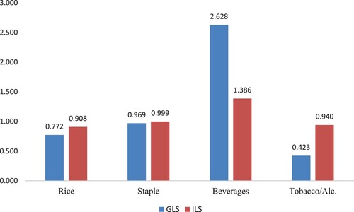
Furthermore, the estimation of income elasticity for staple food relatively yields the same value in both GLS and ILS approaches. The results of the estimated income elasticity of 0.97–0.99. This shows that the income elasticity for staple food is unitary. One percent increase in income will increase staple food consumption by approximately one percent.

An interesting result was income elasticity for beverages. Both the GLS and ILS approaches yield highly elastic estimates of income. The amount of GLS (2.62) is even doubled compared to the estimated ILS (1.38). This finding shows that households will increase their spending on beverages by more than one percent for every one percent of additional income.

Furthermore, estimates of income elasticity for tobacco and alcoholic beverages yield relatively different findings between GLS and ILS. The GLS estimate for this coefficient is 0.42 while the ILS estimate is 0.94. Research by Janda, Mikolášek, and Netuka (2010) in Europe found that the income elasticity for spirits was 0.46 and for wine was 0.75. This finding indicates that poor households do not respond sufficiently to rising incomes to purchase larger amounts of tobacco and alcoholic beverages. Although the share of tobacco and alcoholic beverages is relatively large, poor households do not increase their consumption of these goods when they receive additional income.

Table 6. shows the results of the estimated price elasticity for the four types of goods analysed in the study. Price elasticity of agricultural commodities has become a special study that is widely studied by researchers (Işik and Özbuğday 2021). The estimated price elasticity for uncompensated demand (Marshallian) is relatively higher than the estimated price elasticity for compensated demand (Hicksian). If we look closely, the results of the estimated price elasticity using the GLS approach are very similar to the results of the ILS estimates (except for the uncompensated ILS in the case of tobacco and alcoholic beverages).

Table 6. Estimation of price elasticity: compensated and uncompensated.

	GLS		ILS
	Uncompensated	Compensated	Uncompensated	Compensated
Rice	−0.854	−0.660	−0.861	−0.647
Staple	−0.890	−0.578	−0.913	−0.584
Beverages	−0.890	−0.659	−0.865	−0.716
Tobacco/Alc.	−0.586	−0.466	−0.876	−0.569

Source: STATA output.

The price elasticity of the four types of consumer goods groups is relatively inelastic. It is generally known that the price elasticity of food and beverage is inelastic. When there is an increase in the price of food and beverage goods, the demand for consumption is relatively not reduced much.

It is interesting to study that the price elasticity for tobacco and alcoholic beverages is relatively small compared to the price elasticity of other goods. When the price of tobacco or alcoholic beverages increases, demand for these types of goods decreases slightly. Both the income elasticity and the price elasticity of cigarettes and alcoholic beverages are relatively small. This shows that the changes in consumption due to changes in income and prices are also not too much.

The results of the study generally show that the consumption pattern of the beneficiary households depends on the preferences of each household. Not all cash assistance is used to buy rice or other staple foods. Although more than half of the share of household expenditure is in the form of staple foods, the results of the study show that the largest income elasticity is in the form of beverage products. This means that if there is additional income, poor households will be more sensitive to increasing consumption of various beverages. Allegations that cash transfers will be allocated mostly to tobacco and alcoholic beverages have so far not been strongly substantiated. Of course, there is some additional income spent on cigarettes and alcoholic beverages, but the amount may be small.

Empirical evidence that households receiving cash transfers will spend more additional money on drinks shows that poor households do not always need basic food. Direct gift policies, such as the Rice for Poor Program, may be less effective. Many cases show that households receiving Rice for Poor resell the rice they get in exchange for various goods that they prefer. As a result, the local market is distorted by profit taking behavior.

Instead of giving things that are not necessarily needed, it would be better if they were given cash and let them choose what they wanted more. Economically, the provision of cash assistance will optimally improve household welfare.

Conclusion

Research on the spending patterns of cash transfer recipient households in Indonesia yielded several important findings. First, the biggest expenditure of cash recipient households is for rice and other staple foods. More than half of the expenditures of households receiving cash transfers were used for purchases of rice and other staple foods. Second, research shows that the largest income elasticity is not for staple foods, but for beverage consumption. The implication is that if there is additional income, the portion of spending on beverages is greater than the portion of the increase in income. Third, the price elasticity for all types of consumption goods analysed is inelastic. This means that increasing of price do not have much effect on the consumption of food or beverages.

This finding has several implications. Beneficiary households will prefer to receive cash in order to spend additional money on needs that they think are more suitable. Compared to the basic food aid model, cash transfers are more flexible and can improve household welfare more optimally. Cash transfers may be used to purchase cigarettes or alcoholic beverages. However, the results show that the income elasticity for cigarettes and alcoholic beverages is the lowest.

Therefore, several policy recommendations were proposed. First, the policy of providing cash assistance to poor households can be continued because it has the potential to increase household welfare optimally. Second, the government must support a study on the spending patterns of beneficiary households to anticipate changes in household preferences for consumer goods. Third, the provision of assistance to poor households must also be accompanied by education about choosing healthy food consumption for poor households.

Disclosure statement

No potential conflict of interest was reported by the author(s).

Additional information

Funding

Lembaga Penelitian dan Pengabdian Masyarakat Universitas Trunojoyo Madura, Indonesia under grand number 3121/UN46.4.1/PT.01.03/2021.

References

- Ansah, I. G. K., E. Marfo, and S. A. Donkoh. 2020. “Food Demand Characteristics in Ghana: An Application of the Quadratic Almost Ideal Demand Systems.” Scientific African 8: e00293. doi:10.1016/j.sciaf.2020.e00293.
- Asian Development Bank. 2019. The Social Protection Indicator for the Pacific: Assessing Progress (Issue July). www.adb.org.
- Aung, T., R. Bailis, T. Chilongo, A. Ghilardi, C. Jumbe, and P. Jagger. 2021. “Energy Access and the Ultra-Poor: Do Unconditional Social Cash Transfers Close the Energy Access Gap in Malawi?” Energy for Sustainable Development 60: 102–112. doi:10.1016/j.esd.2020.12.003.
- Banks, J., R. Blundell, and A. Lewbel. 1997. “Quadratic Engel Curves and Consumer Demand.” Review of Economics and Statistics 79 (4): 527–539.
- Barany, L. J., I. Simanjuntak, D. A. Widia, and Y. R. Damuri. 2020. Socio-Economic Assistance in the Midst of the COVID-19 Pandemic. Centre for Strategic and International Studies, April, pp. 1–11. https://www.csis.or.id/publications/bantuan-sosial-ekonomi-di-tengah-pandemi-covid-19-sudahkah-menjaring-sesuai-sasaran.
- BPS. 2013. Indonesian Population Spending and Consumption Patterns, 2013.
- Colen, L., P. C. Melo, Y. Abdul-Salam, D. Roberts, S. Mary, and S. Gomez Y Paloma. 2018. “Income Elasticities for Food, Calories and Nutrients Across Africa: A Meta-Analysis.” Food Policy 77: 116–132. doi:10.1016/j.foodpol.2018.04.002.
- Conrad, Z., L. Jahns, and J. N. Roemmich. 2018. “Study Design for a Clinical Trial to Examine Food Price Elasticity among Participants in Federal Food Assistance Programs: A Laboratory-Based Grocery Store Study.” Contemporary Clinical Trials Communications 10: 154–160. doi:10.1016/j.conctc.2018.05.011.
- Deaton, A., and J. Muellbauer. 1980. “An Almost Ideal Demand System.” The American Economic Review 70 (3): 312–326. http://www.jstor.org/stable/1805222%5Cnhttp://www.jstor.org/stable/1805222?seq=1&cid=pdf-reference#references_tab_contents%5Cnhttp://about.jstor.org/terms.
- Elzaki, R., M. Yunus Sisman, and M. Al-Mahish. 2021. “Rural Sudanese Household Food Consumption Patterns.” Journal of the Saudi Society of Agricultural Sciences 20 (1): 58–65. doi:10.1016/j.jssas.2020.11.004.
- Handa, S., L. Natali, D. Seidenfeld, G. Tembo, and B. Davis. 2018. “Can Unconditional Cash Transfers Raise Long-Term Living Standards? Evidence from Zambia.” Journal of Development Economics 133: 42–65. doi:10.1016/j.jdeveco.2018.01.008.
- Hansen, C. B. 2007. “Generalized Least Squares Inference in Panel and Multilevel Models with Serial Correlation and Fixed Effects.” Journal of Econometrics 140 (2): 670–694. doi:10.1016/j.jeconom.2006.07.011.
- Haushofer, J., and J. Shapiro. 2016. “The Short-Term Impact of Unconditional Cash Transfers to the Poor: Experimental Evidence from Kenya.” The Quarterly Journal of Economics Advance 131 (4): 1973–2042. doi:10.1093/qje/qjw025.
- Hjelm, L., S. Handa, J. de Hoop, and T. Palermo. 2017. “Poverty and Perceived Stress: Evidence from Two Unconditional Cash Transfer Programs in Zambia.” Social Science & Medicine 177: 110–117. doi:10.1016/j.socscimed.2017.01.023.
- Işik, S., and F. C. Özbuğday. 2021. “The Impact of Agricultural Input Costs on Food Prices in Turkey: A Case Study.” Agricultural Economics (Czech Republic) 67 (3): 101–110. doi:10.17221/260/2020-AGRICECON.
- Janda, K., J. Mikolášek, and M. Netuka. 2010. “Complete Almost Ideal Demand System Approach to the Czech Alcohol Demand.” Agricultural Economics 56 (9): 421–434. doi:10.17221/117/2009-agricecon.
- Kratena, K., and M. Wüger. 2010. “The Full Impact of Energy Efficiency on Households’ Energy Demand.” Journal of Food System Research 17 (3): 159–275.
- Labandeira, X., J. M. Labeaga, and M. Rodríguez. 2006. “A Residential Energy Demand System for Spain.” The Energy Journal 27 (2): 87–111. doi:10.5547/ISSN0195-6574-EJ-Vol27-No2-6.
- Lecocq, S., and J. M. Robin. 2015. “Estimating Almost-Ideal Demand Systems with Endogenous Regressors.” Stata Journal 15 (2): 554–573. doi:10.1177/1536867x1501500214.
- Li, J., and R. E. Just. 2018. “Modeling Household Energy Consumption and Adoption of Energy Efficient Technology.” Energy Economics 72: 404–415. doi:10.1016/j.eneco.2018.04.019.
- Moffatt, P. G. 2012. “A Class of Indirect Utility Functions Predicting Giffen Behaviour.” Lecture Notes in Economics and Mathematical Systems 655: 127–141. doi:10.1007/978-3-642-21777-7_10.
- Natali, L., S. Handa, A. Peterman, D. Seidenfeld, and G. Tembo. 2018. “Does Money Buy Happiness? Evidence from an Unconditional Cash Transfer in Zambia.” SSM - Population Health 4: 225–235. doi:10.1016/j.ssmph.2018.02.002.
- Nganau, J. P. 2011. Estimation of the Parameters of a Linear Expenditure System (LES) Demand Function for a Small African Economy (No. 31450; Munich Personal PePEc Archive, Issue 31450).
- Poi, B. P. 2008. “Demand-System Estimation: Update.” The Stata Journal 8 (4): 554–556.
- Poi, B. P. 2012. “Easy Demand-System Estimation with Quaids.” The Stata Journal 12 (3): 433–446. doi:10.1177/1536867x1201200306.
- Rasyid, M., A. Kristina, Sutikno, Sunaryati, and T. Yuliani. 2020. “Poverty Conditions and Patterns of Consumption: An Engel Function Analysis in East Java and Bali, Indonesia.” Asian Economic and Financial Review 10 (10): 1062–1076. doi:10.18488/journal.aefr.2020.1010.1062.1076.
- Schulte, I., and P. Heindl. 2016. “Price and Income Elasticities of Residential Energy Consumption in Germany: The Role of Income and Household Composition.” ZEW Discussion Paper, 16–052(16).
- Sheng, T. Y., M. N. Shamsudin, Z. Mohamed, A. M. Abdullah, and A. Radam. 2008. “Complete Demand Systems of Food in Malaysia.” Agricultural Economics 54 (10): 467–475. doi:10.17221/279-agricecon.
- SMERU. 2006. Evaluation of the Unconditional Cash Transfer in Indonesia. December, 1–4.
- Strauss, J., F. Witoelar, and B. Sikoki. 2016. The Fifth Wave of the Indonesia Family Life Survey: Overview and Field Report: Volume 1. In Rand Labor and Population (Vol. 1, Issue March). doi:10.7249/wr1143.1.
- Vargas-Lopez, A., C. Cicatiello, L. Principato, and L. Secondi. 2021. “Consumer Expenditure, Elasticity and Value of Food Waste: A Quadratic Almost Ideal Demand System for Evaluating Changes in Mexico During COVID-19.” Socio-Economic Planning Sciences, 101065. doi:10.1016/j.seps.2021.101065.
- World Bank. 2017. Towards a Comprehensive, Integrated, and Effective Social Assistance System in Indonesia. doi:10.1596/28850.
- Yaseen, M. R., I. Mehmood, and Q. Ali. 2014. “Comparative Analysis of the Food and Nutrients Demand in Developing Countries: The Case of Main Vegetable Products in South Asian Countries.” Agricultural Economics (Czech Republic) 60 (12): 570–581. doi:10.17221/28/2014-agricecon.