Quantitative assessment of full field deformation of right ventricle during open heart surgery

ABSTRACT

A mathematical method is introduced for quantifying full field deformation images of right ventricle (RV) of the heart. These images are acquired from the RV of the heart during open-heart surgery and analysed using digital image correlation (DIC). The high degree of complexity of the deformation of the heart, especially for the patients who require heart surgery emphasises the importance of a method to analyse the visible section of the surface of the RV. This is difficult with conventional heart-monitoring methods, which rely on describing the overall deformation of the area of interest by measuring the deformation between two points only and discarding all other relevant information contained in the area of interest. In this work, we decomposed the full field deformation images of the visible section of RV into shape descriptor vectors and used the Euclidian distance between two shape descriptor vectors obtained from the reference image and the analysed image to quantify the full field deformation by a single number. The Euclidian distance was used to compare the motion and deformation state of the heart at various stages during the operation. We demonstrate that the Euclidian distance is a more robust indicator describing the overall function of the heart than an individual strain value, especially in case of poor-quality images from which the strain is derived.

KEYWORDS:

• Human biomechanics
• heart muscle
• DIC
• deformation
• motion
• biomaterial characterisation
• image processing

Introduction

Monitoring and analysing the functions of the heart is an important aspect of open-heart surgery. Since the functions of the heart are closely related to its deformation and movements (Smiseth et al. 2016), various echocardiography methods have been developed to measure and analyse the movements, deformation, strain, and strain rate of the heart (Dandel et al. 2009). These methods include Tissue Doppler Imaging (TDI) (Sutherland et al. 1999; Krishna and Thomas 2015) and Speckle Tracking Echocardiography (STE) (Blessberger and Binder 2010; Bansal and Kasliwal 2013). While these methods have their own set of advances and shortcomings (Teske et al. 2009), what they have in common is that they can only take into account the deformation on a planar area (2D deformation). In reality, the heart deforms in a rather complex manner, and there are significant out of plane movements and rotations that are difficult to analyse from a 2D image. Additionally, TDI and STE results are limited to pre-selected areas/directions of the heart that are chosen before the measurements. Consequently, only a portion of the potential data is available for analysis at a time. However, the deformation of the heart is very complex and far from uniform. This fact is even more exacerbated when the heart of the sick patient is already functioning in a non-optimal manner, therefore necessitating the surgery in the first place. During the open-heart surgery and cardiopulmonary bypass (CPB), the functions of the heart are temporarily performed by the CPB circuit. After the surgical repairs and during the weaning process, the heart resumes its functionality and therefore, the deformation of heart is far from normal. This high complexity in deformation of the heart necessitates the study of the full field deformation over the visible section of the ventricle or atrium. While this area does not fully cover the entire RV, it is usually enough to represent the RV movement. The deformation is most likely very anisotropic and non-uniform, but it still is a common practice to describe the function of the RV by a single scalar strain value. For example, the modern ultrasound techniques typically use segmentation to analyse strains of different parts of the heart, but the strain itself is a simple engineering strain that describes only the deformation between two selected points and ignores information encoded in all other image points.

We previously have demonstrated that Digital Image Correlation (DIC) can be an effective tool for analysing the deformations of the right ventricle (RV) of the heart (Soltani et al. 2018). DIC is an image analysis method that relies on visual access to the target surface. Consequently, using DIC to monitor the deformation of the RV is possible because this section of the heart is visible during an open-heart surgery. In its simplest form, DIC measures the displacement by tracking features across the target surface in consecutive images (Planca et al. 2015). DIC can generate displacement vectors at such high spatial resolution that in practice, the analysis produces a full field deformation image of the selected area of interest. Since the full field deformation images can contain the deformation information of each pixel in the entire region of interest, it is virtually impossible to quantitatively analyse the differences between two deformation images or to quantitatively interpret the changes in several consecutive full field deformation images of the target. By visually inspecting these full field deformation images, one can generally perceive the differences and changes from one image to other, but obviously it is not scientifically quantifiable.

Orthogonal decomposition techniques such as Zernike (Teague 1980) and Tchebichef (Mukundan et al. 2001) are emerging methods for quantifying the deformation field images. Orthogonal decomposition decomposes the high-resolution images into shape descriptors that can then be used to reconstruct the original image. Usually a higher number of such shape descriptors leads to better reconstruction of the original images with fewer errors. This reliable method can quantify an image with a manageable number of numerical data. The shape descriptors can be considered as a vector that typically has relatively low number of elements. If one considers two images that are decomposed into shape descriptor vectors, the vectors are quite similar if the two images were originally similar, but if the images are very different, then the resulting vectors are different as well. The difference between the two shape descriptor vectors can be quantified by simply calculating the mathematical distance between the two vectors. This distance is called the Euclidian distance and it can be used to quantify the differences between various images by a single number. The Euclidian distance includes the information from the whole image that was input into the decomposition process (Figure 2(a)). The viability of this process has already been represented in a few studies. For example, Sebastian et al. (Sebastian et al. 2012) validated the orthogonal decomposition for modelling deformation field of a few sample tensile tests. In a more practical study, Christian et al. (Christian et al. 2018) used the same method to assess the strain field in DIC images of a composite material.

Figure 1. Speckle patterns applied to the two cases used in this work

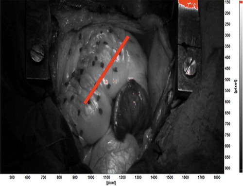
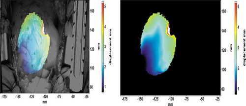
Figure 2. Displacement field map of the heart (a) overlaid on the original image and (b) without the background

The aim of this work is to develop and demonstrate a methodology based on the orthogonal image decomposition for the quantitative analysis of the mechanical behaviour and functionality of the RV during open-heart surgery. The images were obtained, and image analysis was used at different stages during the operation to compare the movements and deformation of the heart. The results show the potential of a more comprehensive deformation analysis method in the field of heart monitoring. The orthogonal decomposition can fully characterise the deformation of the RV in a concise, robust, and simple manner, which may assist the medical staff to better understand the functions of the heart during and after an open-heart surgery.

Materials and methods

The DIC setup used in this work comprised two 5-megapixel E-lite cameras with 50 mm Nikon lenses. The space directly above the surgery table is highly controlled sterile environment and any interference with it is against regulations. Thus, the DIC cameras were mounted on the side of the surgery table using a custom-made vertical rod, overlooking the patient`s chest at a ~ 65 degrees angle and ~2 metres distance. A comprehensive description of the test setup, practical limitations, error sources, and several examples can be found in our previous publication (Soltani et al. 2018).

The target surface needs to have a random high-contrast speckle pattern (Jones and Ladicola 2018). Since in most cases the heart of the patients is covered with a thin layer of fat, the natural contrast of the heart does not provide enough contrast for DIC image analysis (Ruixiang et al. 2017). In this work the surface of the heart was patterned with random dots applied using a non-toxic medical marker (Methylene blue). This pattern is a compromise between accurate DIC measurements, and the practical limitations imposed by the environment. The ink must be sterile and non-toxic, and applying the pattern must not interfere with the medical procedure too much. Figure 1 shows an example of such pattern for one of the surgeries of this study. In our previous work, we have presented details of the application of the pattern, the effect of the pattern quality on the spatial and strain resolution of the measurements and discussed the changes of the pattern quality between different stages of the surgery. For further details please see (Hokka et al. 2015a; Soltani et al. 2018).

The coarse contrast pattern shown in Figure 1 necessitates the use of large subsets. The displacement vectors are calculated by dividing the original image into smaller subset images and tracking the movement of the subsets in consecutive images. The subset must contain enough distinguishable image data so it can be reliably identified in the consecutive images. Therefore, if the contrast pattern is coarse, or the dots are big and far from each other, then the size of the subset must be also large enough so that it includes at least three identifiable features (Jones and Ladicola 2018). The spatial resolution of the DIC also depends on the size of the subset, and the resolution decreases with larger subsets. Even if one places a subset at each pixel location, the large subsets will simply overlap significantly, and they will largely contain the same image data. Therefore, the independent displacement measurements can only be obtained from subsets that are separated from each other by a distance, which increases with the size of the subset. The subset may also deform and rotate between the images. Mathematically this can be considered by using shape functions that allow the shape of the subset to change between the images. Large subsets are prone to nonlinear deformations inside the subsets, and therefore the use of mathematically more complex shape functions is required (Jones and Ladicola 2018). Using a second order nonlinear shape functions significantly improves the strain resolution and reduces the negative impact of the increasing subset size on the spatial resolution (Ruixiang et al. 2017). For full mathematical description of the subset tracking and the shape functions, please refer to (Sutton et al. 2009).

This paper presents the results of the open-heart surgery from two patients as examples of the proposed image analysis method. Our goal is not to give in-depth medical relevance nor statistically meaningful data on the conditions of the patients, but to demonstrate the benefits of the new method with data obtained from two randomly selected patients. The patients involved in the study gave written consent acknowledging their participation and receiving the information regarding the risks of the study. The study protocol was reviewed and approved by the European Union Drug Regulating Authorities Clinical Trials (2016–000575-24). Both surgeries were imaged during three stages: Native (after sternotomy), Post-cardiopulmonary bypass or CPB (after the repairs of the heart), and inotrope (a theophylline bolus to increase the contraction force of the heart). During each stage, a sequence of approximately 200 images was recorded, which corresponds to approximately 15 heartbeats. Images were analysed offline using LaVision Davis 8.4 software. Table 1 shows how the DIC calculations were carried out. The longitudinal strain of the right ventricle was measured across the visible surface of the heart using a virtual extensometer. The strain presented in this paper is the engineering strain, which is the change in the length of the virtual extensometer divided by its original length in the first (reference) image. This definition of strain is too simple on its own to describe the complex full field deformation and motion of the heart, as will be demonstrated later in this paper. The engineering strain, however, is typically used in the ultrasound technology, and therefore, it was used in this work as a ‘reference’ or standard strain definition. Majority of the results presented in this work focus on the analysis of the full field displacement data.

Table 1. DIC analysis details

Imaging frequency	15–20 Hz
Subset size	79 pixels
Subset shape function	Nonlinear 2^nd order
Step size	10 pixels
Pixel size	~0.03 mm
Calibration error	~0.1 mm
Interpolation method	6th order spline function
Strain calculation method for engineering strain	Virtual extensometer
Displacement calculation method	Sum of differentials
Reference frame	A new reference frame was selected for each heartbeat

The quantitative comparison of the deformation of the heart in different images was carried out using the full field displacement field images. The displacement information, or the length of the displacement vector, does not depend on the orientation of the cameras or the selected coordinate system. Figure 2 shows an example of a displacement field overlaid on the original image (Figure 2(a)) and with a simple black background (Figure 2(b)). The example is from the native stage of surgery#1, and it shows an average deformation of 100 mm during the expansion phase of heartbeat (diastole). The displacement field images with only the displacement information (without the background image) were used for the orthogonal decomposition.

The decomposition of the displacement images was done using a Matlab-based software originally developed by Patterson and Christian (Christian and Patterson 2018). The software decomposes the input image into Tchebichef polynomials and returns the polynomial vector for further processing. The detailed mathematical description of the process is provided in detail in Mukundan et al. (2001), and only a brief summary is given here to help the readers. Using a series of Tchebichef polynomials $T\left(i,j\right)$ the displacement image $I\left(i,j\right)$ is decomposed into:

(1) $I\left(i,j\right)=\sum _{k=0}^N{s}_{k}I\left(i,j\right)$(1)

Where the coefficients $s_k$ is:

(2) $s_k=\sum _{i,j}^{n}I\left(i,j\right)T_k\left(i,j\right)$(2)

Here s_k is the shape vector of I(i,j), n is the number of data points in the displacement field, and N is the selected number of shape descriptors. The shape descriptors describe the decomposed images quantitatively, and they can also be used to reconstruct the original image. Therefore, the difference in the moments can be used to quantitatively describe the difference between two images. If the image descriptors are simply used as vectors, the Euclidian distance between two shape descriptor vectors describing two images can be used to quantitatively describe the differences between the two images. If the images are very similar, then the moment vectors are very similar, and therefore the Euclidian distance is very small. On the other hand, if the images are very different, the Euclidian distance describing the difference between the two images will increase as well. The Euclidian distance d between two shape descriptor vectors p and q in the N-dimensional space can be calculated as:

(3) $d\left(p,q\right)=\sqrt{\sum _{i=1}^N{\left(p_i-q_i\right)}^2}$(3)

The quality of the decomposition process can be evaluated by reconstructing the image using intensity shape descriptors. The accuracy of decomposition process can be assessed by comparing the intensities of the original image with the reconstructed images:

(4) $Er=\sqrt{\frac{1}{n}\sum _{i,j}^n{\left(\text{^}I\left(i,j\right)-I\left(i,j\right)\right)}^2}$(4)

Here n is the number of original images, $\text{^}I\left(i,j\right)$ is the intensity of a pixel in the reconstructed and $I\left(i,j\right)$ the intensity in the original image. For a more detailed description of Equations 1 to 4 please refer to ref. (Sebastian et al. 2012). Any E_r greater than 3 is an indication of poor reconstruction process. The E_r is directly influenced by the number of decomposition shape descriptors (N), with higher values resulting in better reconstruction result and lower errors.

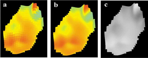
The decomposition of the displacement images can use raw, smoothed or greyscale images as a source. The smoothing process for the smoothed images consists of applying a bilinear interpolation between the neighbouring vectors when available. Average value of available vectors is used when any are missing. Figure 3(a–c) shows the raw, smoothed and greyscale displacement field images for the native stage of surgery #2.

Figure 3. Displacement field images (a) raw (b) smoothed (c) greyscale

Results and discussion

Figure 4 shows the Euclidian distance obtained for several heartbeats for the smoothed, non-smoothed, and greyscale displacement images. The full field displacement image includes a very comprehensive description of the motion and deformation of the heart, but the quantitative comparison of two images is very difficult. The Euclidian distance between two image descriptor vectors describes the difference between the two by one single numerical value. For a single heartbeat, the first full field displacement image in the series can be used as the reference, and the rest of images in the sequence are compared to this image. Since the movement of the heart in one heartbeat is always somewhat cyclic, the reference or the first image should look very much like the last image. In one heartbeat, the displacement fields of the first and the second images are only slightly different, and thus the Euclidian distance is small. The difference between the displacement fields increases to a maximum value corresponding to the maximum contraction (end systole). As the heart relaxes and expands again towards the diastole, the displacement field images become more like the original reference image, leading to the Euclidian distance becoming smaller and eventually close to zero.

Figure 4. (a)The Euclidian distance as a function of input image number of smoothed, non-smoothed and greyscale images for the native stage of the surgery #1 (b) The Er values as a function of input image number of smoothed, non-smoothed and greyscale images for the native stage of the surgery #1

At all stages and for both surgeries, the Euclidian distance obtained from the greyscale images shows higher peak values for each heartbeat compared to the data obtained from the smoothed and non-smoothed colour images. An example of this is shown in Figure 4(a) which contains the Euclidian distance as a function of image number for the smoothed, non-smoothed and greyscale image data for the native surgery stage of patient #1 with 21 shape descriptors. The Euclidian distance for the smoothed and non-smoothed images shows very similar peak values and overall behaviour. The values of the E_r describing the quality of the decomposition process for all three input variants for all decomposed images are between ~0.06 and 0.2, thus showing good correlation between the original and reconstructed images. Figure 4(b) shows an example of error values for each image type shown in Figure 4(a). Overall, the pre-processing of the input image does not seem to have a very strong effect on the Euclidian distance calculation, and the comparison of the images seems very robust. The greyscale images, however, do show a slightly higher sensitivity, as the Euclidian distance of the greyscale images changes more during one heartbeat than the Euclidean distance of the colour images of the same heartbeat. Thus, the greyscale displacement images may be more sensitive to observe small differences in the overall behaviour of the heart. This is in accordance with a well-known phenomenon in the digital image processing field, where greyscale images are less prone to noises and artefacts as the result of digital compression of data (Christian and Patterson 2018).

Figure 5(a,b) shows the effect of increasing the number of shape descriptors on the average of the highest Euclidian distance observed in the four heartbeats for patient #1 and #2, respectively. For both patients, increasing the number of the shape descriptors from two to 21 is accompanied by an increase of ~0.1–0.2 in average peak values. However, if the number of shape descriptors is increased to from 21 to 121 and 221, the average peak values barely change. The change in the E_r values are more pronounced when the number of the shape descriptors increases. Regardless of the stage of the surgery, the E_r of the decomposition process decreases on the average from ~0.3 to 0.1 when the number of shape descriptors increases up to 121 and stays the same for an increase to 221 shape descriptors.

Figure 5. Average of the highest Euclidian distance for four heartbeats obtained with 2, 21, 121 and 221 shape descriptors for (a) surgery #1 and (b) surgery #2

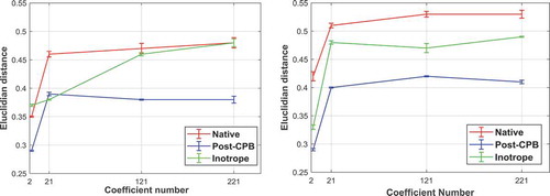
If only two shape descriptors are used, the peak Euclidian distance is lower in the native stage compared to the same images being decomposed with 21 or more shape descriptors. This is also similar for the Post-CPB and inotrope stage measurements. Therefore, it is quite obvious that using 21 shape descriptors significantly improves the sensitivity of the analysis, but on the other hand, using more than 21 shape descriptors does not improve the sensitivity much more.

The peak Euclidian distance values describe essentially the difference between the deformation at maximum volume of the heart and the deformation at minimum volume after the systolic compression stage. Therefore, higher peak values indicate larger global deformation. Since the cardiac functions are highly complex, any change in the deformation of myocardium could be the result of abnormal functionality of the heart. In turn, the change in the deformation of the heart is directly related to parameters such as ejection fraction and volume change in each cycle among other ones, as these parameters play an important role in describing the functionality of the heart. Consequently, Euclidian distance values, which have the potential to act as a direct correlation to the deformation of the entire visible section of the heart, could also be used to assess the functionality of the heart given that enough such data are available to establish the correlation. Of course, the deformation of the heart is very anisotropic (Soltani et al. 2019), which could result in localised expansion or contraction in the displacement field images of the heart at the same volume. Thus, the Euclidian distance values of the two different states of the heart at the same volume could potentially be similar, despite localised deformation being different between the two. The Euclidian distance values describe the global deformation and motion, while the strain measurements describe the localised deformation of the heart. Considering the fact that in the mechanical analysis of the function of the heart, the changes in the deformation behaviour of the heart are of much more importance than the absolute values (Ho and Solomon 2006), quantifying the global deformation stage of the heart has the potential to provide information and indications of irregularities in the movements, deformation patterns, and mechanical functions of the heart.

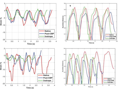
Figure 5(a,c) shows the engineering longitudinal strain as a function of time for the three imaging stages for the patients #1 and #2, and Figure 5(b,d) show the Euclidian distance calculated for the same image sequences, respectively. The Euclidian distance is calculated using the greyscale images and 21 shape descriptors. The red line inFigure 1 shows the location, direction, and length of the virtual extensometer used for strain measurements. While each heartbeat can be clearly identified from the strain data (Figure 5(a,c)), the shape of each cycle and the peak values vary from heartbeat to heartbeat. This is more evident for the data obtained for the patient #2, where for example, the inotrope stage cycles seem quite irregular. This inconsistency in the strain data is most likely related to the fact that the location of the virtual extensometer could be in the area that contains high number of calculation errors. The location of the virtual extensometer is chosen in the reference image, and even if this is done extremely carefully placing the extensometer in an area with very low surface reconstruction (epipolar) errors, the same location may have high errors in the consecutive images of the sequence. Therefore, it is almost impossible to select a position of the virtual extensometer that always produces high-quality strain data in a sequence of 50 or more images. After all the image quality in these challenging imaging conditions is average at best. Finally, the displacements are calculated as the sum of differentials or as a sum of differential displacements between consecutive images. Consequently, the errors will accumulate as the calculations advance in the sequence of images. For poor image quality and coarse patterns, this calculation method is significantly more robust than comparing the nth image to the reference image. Finally, the virtual extensometer only returns the relative length of the line, or the relative motion of the start and end points of the extensometer line. Therefore, it uses only two subset images to describe the strain of the heart and discards all other strain and displacement information decoded in the image. The image decomposition shape descriptors and the Euclidian distance, on the other hand, include the information of the whole full field displacement image.

The variations in both the overall shape of the plot and the maximum peak strain values are not so apparent in the Euclidian distance plots as they are in the strain plots. As shown in Figure 5(b,d) each cycle is very well defined and the peak values are relatively the same from one cycle to another. For the patient #1, the peak Euclidian distance decreases from native to Post-CPB stage while increasing again at the Inotrope stage (Figure 5(b)). This is not so clearly observed in the strain data (Figure 5(a)). Although there are cycles where strain peak values for the native stage are higher– (second and third heartbeats), the peak strain values for the Post-CPB are generally higher than in the Inotrope stage. The Euclidian distance for the patient #2 (Figure 5(d)) is similar to those observed for the patient#1. The Euclidian distance drops in the Post-CPB stage and then increases again after the Inotrope (Native, inotrope and post-CPB). The same is somewhat true for the strain data shown in Figure 5(c). However, the strain data are more irregular compared to the strain Data obtained for patient#1, especially for the Inotrope stage where the cycles are barely distinguishable.

Figure 6. (a) Engineering strain and (b) Euclidian distance as a function of time for patient#1 and (c) engineering strain (d) Euclidian distance as a function of time for patient#2

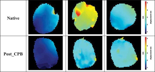
Figure 7 shows comparison of the images in the native and post-CPB stages. The comparison is shown as the Euclidian distance obtained as the distance between the shape descriptor vector of an image of the native stage and the corresponding image of the post-CPB stage (Delta Euc.). For example, the first image of the sequence in the Native stage is compared to the first image of the sequence of the Post-CPB sequence. The first image in each of the sequences is very similar to each other, and the Euclidian distance is therefore similar. In the further images, the Euclidian distance will either increase or remain the same depending if the displacement fields are similar or different in the consecutive images. Figure 8 shows an example of this behaviour. The first image of the native stage (Figure 8(a)) is similar to the corresponding image in the post-CPB stage (Figure 8(d)). The same applies to the last image of the cycle for the native (Figure 8(c)) and post-CPB stage (Figure 8(f)). Consequently, the Delta Euc. values for these two image pairs are close to zero. However, the displacement image for the end-diastole state have vastly different colour schemes between the native (Figure 8(b)) and post-CPB (Figure 8(e)) stages, which leads to a higher Delta Euc. value of ~0.25. Some manual adjustments were made to the image sequences to have the same number of images in the native stage and in the post-CPB stage image sequence. For example, the image sequences of the patient #1 included 78 images in the native stage and 61 in the post-CPB stage. Consequently, the number of images had to be reduced by discarding a few data points during each cycle for the stage with the higher number of images. This was done by matching the maximum Euclidian distance in both image sequences and reducing some redundant images from the longer image sequence. If the displacements of the heart in the Native and Post-CPB stages were similar, the Euclidian distance between the two image sequences would be close to zero for all images. The Calculation of the Euclidian distance between the images in the two stages of the surgery reveals any changes in the displacements of the heart. Therefore, it can be considered ‘differential’ analysis, which is a quantitative measure for the effects of the surgical repairs, medicine, ventilation settings, or other change that occurs during the surgery.

Figure 7. Euclidian distance between native and post-CPB stages as the function of image number for (a) patient#1 (b) patient#2

Figure 8. Displacement field images of the surgery #1 (a) Image number 10 of native stage, (b) Image number 15 of native stage, (c) Image number 17 of native stage, (d) Image number 10 of post-CPB stage, (e) Image number 15 of post-CPB stage, and (f) Image number 17 of post-CPB stage

Conclusions

A mathematical image decomposition method was used to quantify the high-resolution full field displacement images acquired from DIC analysis. Based on the results the following conclusions can be summarised:

• The poor image quality of the acquired images is a major source of technical and practical difficulties in using DIC to measure the deformation of the heart. Some of these difficulties can be overcome by using controlled lighting in the surgery room and using a fixed DIC setup which contains cameras in a housing at fixed location. This way the cameras can be calibrated outside the surgery environment with the only variable being the distance between the entire setup and the subject of analysis.

• Decomposing these images into vectors makes it possible to compare the state of the deformation of the RV by calculating the Euclidian distance between two images.

• The decomposition method mitigates the negative effects of the technical and practical problems encountered in DIC analysis of deformation of the RV.

• Comparing the images of a single heartbeat to the first image of that heartbeat gives an estimate of the absolute deformation of the heart. The Euclidian distance in this instance describes the differences between the deformation at maximum and minimum volume states of the heart in a single heartbeat.

• Comparing images of heartbeats obtained at different stages of the surgery, for example images of a heartbeat of the Native stage to the images of a heartbeat of the Post-CPB gives a differential analysis of the change in deformation pattern of the heart. If the Euclidian distance is zero, then the global deformation of the heart has not changed during the surgery, but a higher value of the Euclidian distance indicates stronger change in the global deformation of the RV. This analysis also indicates when the differences occur, e.g., during systole or diastole.

• The Euclidian distance could be used as an index describing the global mechanical responsiveness and the change in deformation behaviour of the RV. This, however, requires much more work and needs to be confirmed for a broader number of patients than what was used in this work only aiming at demonstrating the new image analysis methodology.

Disclosure statement

No potential conflict of interest was reported by the author(s).

Additional information

Notes on contributors

A. Soltani

Ayat Soltani has gotbachelor degree from Azad University of Ahavaz/Iran. After spending 2 years working as an NDT inspector I decided to return to the academy. I finished my M.Sc. studies in 2013 at Tampere University and spent two years working on a printed electronics project. After two years,  I returned to Material Science Department as a PhD student, and started to work on the application of Digital Image Correlation to study the deformation of the heart during open-heart surgeries.  This includes imaging the visible section of the heart after the sternotomy and analysing the myocardial deformation in-vivo.

J. Lahti

Juha Lahti graduated as an anaesthesiologist from Tampere university in 2015. After finishing his residency in Jorvi hospital, he started working as an anaesthesiologist in Cardiac surgeries in Tampere Hospital in 2010. He is currently working on acquiring his doctorate and researching the relevancy of Digital Image Correlation analysis in monitoring the functions of the heart from a medical point of view. 

K. Järvelä

Kati Järvelä is working at Tampere Hospital as a Doctor of Medicine and a Specialist in Anaesthesiology. She acted as an advisor to the research involved in this paper and is currently collaborating with the rest of medical staff to write a follow up paper.

J. Laurikka

Jari Laurikka is a Cardiac surgeon and has worked at Tampere Hospital since its establishment in 2004.  In addition to the chief physician of the Cardiac Hospital, he is a professor of cardiac and thoracic surgery at the Faculty of Medicine and Life Sciences of the University of Tampere. The work in this paper was his first venture into working in a multidisciplinary research project which hopefully will lead into future innovation in the field of heart monitoring.

M. Hokka

Mikko Hokka is a professor at Tampere University and the head of Impact research group. His latest work is focused on digital image analysis and infrared imaging, while hoping to utilize the unique abilities of these methods to bridge the gap in understanding of how the microscopic material behavior connects with the larger macroscopic behavior.

References

- Bansal M, Kasliwal R. 2013. How do I do it? Speckle-tracking echocardiography. Indian Heart J. 65(1):117–123. doi:10.1016/j.ihj.2012.12.004.
- Blessberger H, Binder T. 2010. Two dimensional speckle tracking echocardiography: basic principles. Heart. 96:716–722. doi:10.1136/hrt.2007.141002.
- Christian WJ, DiazDelaO FA, Patterson EA. 2018. Strain-based damage assessment for accurate residual strength prediction of impacted composite laminates. Compos Struct. 184:1215–1223. doi:10.1016/j.compstruct.2017.10.022.
- Christian WJ, Patterson EA. 2018. Euclid Ver: 1.01. http://www.experimentalstress.com/software.htm.
- Dandel M, Lehmkuhl H, Knosalla, C, Suramelashvili N, Hetzer R. 2009. Strain and strain rate imaging by echocardiography – basic concepts and clinical applicability. Curr Cardiol Rev. 5:133–148. doi:10.2174/157340309788166642.
- Ho CY, Solomon SD. 2006. A clinician’s guide to tissue Doppler. Circulation. 113(10):396–398. doi:10.1161/CIRCULATIONAHA.105.579268.
- Hokka M, Mirow N, Nagel H, Irqsusi M, Vogt S, Kuokkala V. 2015a. In-vivo deformation measurements of the human heart by 3D digital image correlation. J Biomech. 48:2217–2220. doi:10.1016/j.jbiomech.2015.03.015.
- Jones EM, Ladicola M. 2018. A good practices guide for digital image correlation, international digital image correlation society.
- Krishna KK, Thomas L. 2015. Tissue Doppler imaging in echocardiography: value and limitations. Heart Lung Circ. 24:224–233. doi:10.1016/j.hlc.2014.10.003.
- Mukundan R, Ong SH, Lee PA. 2001. Image analysis by Tchebichef moments. Trans Image Process. 10(9):1357–1364.
- Planca M, Tozzi G, Cristofolini L. 2015. The use of digital image correlation in the biomechanical area: a review. Intc Biomech. 3(1):1–21. doi:10.1080/23335432.2015.1117395.
- Ruixiang B, Hao J, Zhenkun L, Weikang L. 2017. A novel 2nd-order shape function based digital image correlation method for large deformation measurements. Opt Lasers Eng. 90:48–58. doi:10.1016/j.optlaseng.2016.09.010.
- Sebastian C, Hack E, Patterson E. 2012. An approach to the validation of computational solid mechanics models for strain analysis. J Strain Anal Eng Des. 48(1):36–47. doi:10.1177/0309324712453409.
- Smiseth OA, Torp H, Opdah A, Haugaa KH, Urheim S. 2016. Myocardial strain imaging: how useful is it in clinical decision making? Eur Heart J. 37(15):1196–1207. doi:10.1093/eurheartj/ehv529.
- Soltani A, Lahti J, Järvelä K, Curtze S, Laurikka J, Hokka M, Kuokkala V-T. 2018. An optical method for the in-vivo characterization of the biomechanical response of the right ventricle. Sci Rep. 1(8):6831.
- Soltani A, Lahti J, Järvelä K, Laurikka J, Kuokkala V-T, Hokka M. 2019. Characterization of the anisotropic deformation of the right ventricle during open heart surgery. Comput Methods Biomech Biomed Eng. 23(3):103–113 .
- Sutherland GR, Kukulski T, Voight JU, D’hooge J. 1999. Tissue doppler echocardiography. Echocardiography. 16(5):509–520.
- Sutton MA, Oretu J, Schreier HW. 2009. Image Correlation for shape, motion and deformation measurements. New York: Springer.
- Teague MR. 1980. Image analysis via the general theory of moments. J Opt Soc Am. 70(8):920–930.
- Teske A, Robberecht C, Kuiperi C, Nuyens D, Willems R, de Ravel T, Matthijs G, Heidbüchel H. 2009. Echocardiographic tissue deformation imaging quantifies abnormal regional right ventricular function in arrhythmogenic right ventricular dysplasia/cardiomyopathy. J Am Soc Echocardiogr. 22:920–927. doi:10.1016/j.echo.2009.05.014.